Stable solutions of the Yamabe equation on non-compact manifolds

Abstract.

We consider the Yamabe equation on a complete non-compact Riemannian manifold and study the condition of stability of solutions. If $(M^{m},g)$ is a closed manifold of constant positive scalar curvature, which we normalize to be $m(m-1)$, we consider the Riemannian product with the $n$-dimensional Euclidean space: $(M^{m}\times{\mathbb{R}}^{n},g+g_{E})$. And study, as in [2], the solution of the Yamabe equation which depends only on the Euclidean factor. We show that there exists a constant $\lambda(m,n)$ such that the solution is stable if and only if $\lambda_{1}\geq\lambda(m,n)$, where $\lambda_{1}$ is the first positive eigenvalue of $-\Delta_{g}$. We compute $\lambda(m,n)$ numerically for small values of $m,n$ showing in these cases that the Euclidean minimizer is stable in the case $M=S^{m}$ with the metric of constant curvature. This implies that the same is true for any closed manifold with a Yamabe metric.

1. Introduction

Let $(X^{N},h)$ be a complete non-compact Riemannian manifold of dimension $N\geq 3$, without boundary. We consider the $h$-Yamabe functional given by:

$$Y_{h}(u)=\frac{\int_{X}\ \left(a_{N}\|\nabla u\|^{2}+s_{h}u^{2}\right)\ dv_{h}}{(\int_{X}u^{p}dv_{h})^{2/p}}=\frac{E_{h}(u)}{\|u\|_{p}^{2}}.$$

where $a_{N}=\frac{4(N-1)}{N-2}$, $p=p_{N}=\frac{2N}{N-2}$, $s_{h}$ will denote the scalar curvature of the metric $h$ and $dv_{h}$ its volume element. The function $u\neq 0$ is assumed to be in the Sobolev space $L_{1}^{2}(X)$. We will always assume that $(X,h)$ is such that the Sobolev embedding $L_{1}^{2}(X)\subset L^{p}(X)$ holds. This is true for instance if the injectivity radius is positive and the Ricci curvature is bounded below [8, Corollary 3.19].

The Yamabe constant of $(X,h)$ is defined as

$$Y(X,h)=\inf_{u\in L_{1}^{2}(X)-\{0\}}Y_{h}(u).$$

When $s_{g}\geq 0$ this number is always finite (and non-negative) and it is bounded above by the Yamabe constant of $(S^{N},g_{0}^{N})$, where $g_{0}^{N}$ is the metric of constant sectional curvature 1 on $S^{N}$, by the well known local argument of T. Aubin [4].

Although Yamabe constants have been more often considered and are better understood in the case of closed manifolds, the study of the constants for open Riemannian manifolds is also of interest by itself and in connection with the closed case. A general study of Yamabe constants of noncompact manifolds can be found in [7]. See also [1, 2, 13]

Our main motivation is to understand the Yamabe constants of certain non-compact Riemannian manifolds which play a central role in the study of the Yamabe invariants of closed manifolds (in particular when studying how the invariants behave under surgery, see [3]). In the present article we will consider the stability of solutions of the Yamabe equation. A solution $f$ of the $h$-Yamabe equation is a solution of the Euler-Lagrange equation of $Y_{h}$ which means that for each $u\in C_{0}^{\infty}(X)$ the function $H_{u}(t)=Y_{h}(f+tu)$ verifies $H_{u}^{\prime}(0)=0$. The solution $f$ is called stable if for every $u$, $H_{u}^{\prime\prime}(0)\geq 0$. The condition is well understood in the closed case: $f$ being a solution of the Yamabe equation means that $f^{p-2}h$ has constant scalar curvature and it is stable if and only if $s_{f^{p-2}h}\leq(N-1)\lambda_{1}(f^{p-2}h)$, where $\lambda_{1}$ is the first positive eigenvalue of the positive Laplacian of the Riemannian metric. This condition can be expressed also in terms of the original metric $h$, but in the closed case there is no reason to use such expression. A typical situation of interest in the complete noncompact case is a metric of constant positive scalar curvature and infinite volume for which one is interested in computing the Yamabe constant. A solution of the Yamabe equation gives a metric of constant scalar curvature which is non-complete, of finite volume. Since the analysis in such a manifold is not well understood it seems more reasonable to work on the original metric. Therefore we will begin this article by studying the stability condition on a non-compact complete Riemannian manifold of constant positive scalar curvature.

We introduce the following invariant:

Definition 1.1.

Let $(X,h)$ be a complete Riemannian manifold of constant positive scalar curvature and $f\in C_{+}^{\infty}(X)\cap L_{1}^{2}(X)$ be a positive smooth critical point of $Y_{h}$. Let $N(h,f)=\{u\in L_{1}^{2}(X)-\{0\}:\int_{X}f^{p-1}u\ dv_{h}=0\}$ and define

$$\alpha(X,h,f)=\inf_{u\in N(h,f)}\ \frac{E_{h}(u)}{\int_{X}f^{p-2}u^{2}dv_{h}}.$$

With this notation the condition for stability reads:

Theorem 1.2.

Let $(X,h)$ be a complete Riemannian manifold of constant positive scalar curvature and $f\in C_{+}^{\infty}(X)\cap L_{1}^{2}(X)$ be a positive smooth critical point of $Y_{h}$. $f$ is stable if and only if

$$\alpha(X,h,f)\geq(p-1)\frac{E_{h}(f)}{\|f\|_{p}^{p}}.$$

To study stability of solutions of the Yamabe equation on open manifolds one would need to compute the invariant $\alpha$.

The example we will be most interested in is the case $(M^{m}\times{\mathbb{R}}^{n},g+g_{E}^{n})$ where $M^{m}$ is closed and $g$ has constant scalar curvature which we normalize to be $m(m-1)$. One can restrict the functional to functions which depend only on the Euclidean variable and define as in [2]

$$Y_{{\mathbb{R}}^{n}}(M\times{\mathbb{R}}^{n},g+g_{E}^{n})=\inf_{u\in L_{1}^{2}({\mathbb{R}}^{n})-\{0\}}Y_{g+g_{E}^{n}}(u).$$

In [2] $Y_{{\mathbb{R}}^{n}}(M\times{\mathbb{R}}^{n},g+g_{E}^{n})$ is computed in terms of the best constant of the classical Gagliardo-Nirenberg inequality. In particular there is a unique $Y_{{\mathbb{R}}^{n}}$-minimizer $f$ which is a radial, decreasing, smooth function and the scalar curvature of $f^{p-2}(g+g_{E}^{n})$ is $m(m-1)$. It follows that $\frac{E_{h}(f)}{\|f\|_{p}^{p}}=m(m-1)$. In Section 2 we will show that the there is a minimizer for $\alpha(M\times{\mathbb{R}}^{n},g+g_{E}^{n},f)$ and then in Section 4 we will show that it is of the form $a(y)b(x)$ where $-\Delta_{g}a=\lambda_{1}a$, $\lambda_{1}$ is the first positive eigenvalue of $-\Delta_{g}$. Then we see from Theorem 1.2 that :

Theorem 1.3.

Let $(M^{m},g)$ be a closed Riemannian manifold of constant scalar curvature $m(m-1)$ and $f$ the $Y_{{\mathbb{R}}^{n}}$-minimizer normalized so that the scalar curvature of $f^{p-2}(g+g_{E}^{n})$ is $m(m-1)$. $f$ is a stable critical point of $Y_{g+g_{E}^{n}}$ if and only if

(1) $$\inf_{b\in L_{1}^{2}({\mathbb{R}}^{n})-\{0\}}\ \left(\frac{\int_{{\mathbb{R}}^{n}}(a_{N}\|\nabla b\|_{2}^{2}+m(m-1)b^{2})}{\int_{{\mathbb{R}}^{n}}f^{p-2}b^{2}}+a_{N}\lambda_{1}\frac{\int_{{\mathbb{R}}^{n}}b^{2}}{\int_{{\mathbb{R}}^{n}}f^{p-2}b^{2}}\right)\ \geq(p-1)m(m-1)$$

In order to use the previous theorem we will consider the function:

(2) $$\lambda\mapsto A(\lambda)=\inf_{b\in L_{1}^{2}({\mathbb{R}}^{n})-\{0\}}\ \left(\frac{\int_{{\mathbb{R}}^{n}}(a_{N}\|\nabla b\|_{2}^{2}+m(m-1)b^{2})}{\int_{{\mathbb{R}}^{n}}f^{p-2}b^{2}}+a_{N}\lambda\frac{\int_{{\mathbb{R}}^{n}}b^{2}}{\int_{{\mathbb{R}}^{n}}f^{p-2}b^{2}}\right)$$

In section 4 we will prove that $A(\lambda)$ is realized by a radial decreasing function and then deduce the following:

Corollary 1.4.

The infimum is a strictly increasing function of $\lambda$. Therefore there exists a unique value of $\lambda>0$ such that $A(\lambda)=(p-1)m(m-1).$

We introduce the following constant which depends only on the dimensions $m,n$:

Definition 1.5.

The value of $\lambda$ given by the previous corollary will be called $\lambda(m,n)$.

We have

Theorem 1.6.

Let $(M,g)$ be a closed Riemannian manifold of constant scalar curvature $m(m-1)$. Let $\lambda_{1}>0$ be the first positive eigenvalue of $-\Delta_{g}$. Then the metric $f^{p-2}(g+g_{E}^{n})$ is stable if and only if $\lambda_{1}\geq\lambda(m,n)$.

Note that if $g$ is a Yamabe metric (a minimizer for the Yamabe functional) then in particular it is stable and as we mentioned before this means that $\lambda_{1}(g)\geq m$. Therefore we have

Theorem 1.7.

If $m\geq\lambda(m,n)$ then for any Yamabe metric $g$ on the closed manifold $M$ the $Y_{{\mathbb{R}}^{n}}$-minimizer on $(M\times{\mathbb{R}}^{n},g+g_{E}^{n})$ is stable.

The condition on Theorem 1.7 can be checked numerically: a radial mimimizer for $A(\lambda(m,n))$ is given by a solution of the ordinary linear differential equation :

(3) $$u^{\prime\prime}(t)+\frac{n-1}{t}u^{\prime}(t)+\left(\frac{(p-1)m(m-1)}{a_{N}}f^{p-2}-\left(\frac{m(m-1)}{a_{N}}+\lambda(m,n)\right)\right)u(t)=0$$

with $u(0)=1$, $u^{\prime}(0)=0$. In the previous equation replace $\lambda(m,n)$ by a variable $\lambda$. As explained in Section 4 using Sturm comparison theory one can easily check that $\lambda(m,n)$ is the unique value of $\lambda$ such that the solution of previous equation (with the given initial conditions) is positive and decreasing. For $\lambda>\lambda(m,n)$ the solution has a local minimum and for $\lambda<\lambda(m,n)$ has a 0 at finite time. The function $f$ can be computed numerically (see for instance the discussion in [2]) and then for a fixed $\lambda$ one can compute numerically the solution of (3) and check whether $\lambda<\lambda(m,n)$ or $\lambda>\lambda(m,n)$.

In figure (1(c)) we show the solutions of equation (3) for $m,n=2$. In this case one computes $\lambda(2,2)\approx 1.80405...$ and we display solutions with $\lambda>\lambda(2,2)$ and $\lambda<\lambda(2,2)$.

Table 1 gives the numerical computed value of $\lambda_{m,n}$, for low dimensions ($m+n\leq 9$): in these cases one has $\lambda_{m,n}\leq m$.

(a) $\lambda<1.80405$, $u(t)=0$ for some $t>0$.

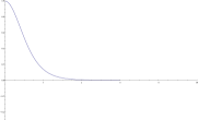
(b) $\lambda_{2,2}\approx 1.80405$, $u$ is always decreasing.

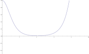
(c) $\lambda>1.80405$, $u$ has a local minimum at some $t>0$.

Figure 1. For dimensions $m,n=2$, we display numerical solutions of equation (3). $\lambda_{2,2}\approx 1.80405$ .

Table 1. Numerical values of $\lambda_{m,n}$

m	n	$\lambda_{m,n}$
2	2	1.8041
3	2	2.9183
2	3	1.6735
2	4	1.5823
3	3	2.8372
4	2	3.9553
2	5	1.5145

m	n	$\lambda_{m,n}$
3	4	2.7669
4	3	3.9023
5	2	4.9718
2	6	1.4459
3	5	2.7070
4	4	3.8506
5	3	4.9348

m	n	$\lambda_{m,n}$
6	2	5.9806
2	7	1.4165
3	6	2.6551
4	5	3.8028
5	4	4.8958
6	3	5.9533
7	2	6.9859

Acknowledgement: The authors would like to thank Prof. Kazuo Akutagawa for many helpful comments on the first version of the article.

2. Yamabe constants of open manifolds

In this section we will discuss some preliminary definitions and results about Yamabe constants on open manifolds. For an open Riemannian manifold $(X^{N},h)$ we consider the $h$-Yamabe functional defined as

$$Y_{h}(u)=\frac{\int_{X}\ (a_{N}\|\nabla u\|^{2}+s_{h}u^{2})\ dv_{h}}{(\int_{X}u^{p}dv_{h})^{2/p}}$$

where the function $u$ is taken to be (non-zero) in $L_{1}^{2}(X)$ and recall that we are assuming that the Sobolev embedding $L_{1}^{2}\subset L^{p}$ holds. The Yamabe constant of $(X,h)$ is then defined as

$$Y(X,h)=\inf_{u}Y_{h}(u)$$

Let $E_{h}(u)=\int_{X}\ (a_{N}\|\nabla u\|^{2}+s_{h}u^{2})\ dv_{h}$ so that $Y_{h}(u)=E_{h}(u)\|u\|_{p}^{-2}$.

A critical point of $Y_{h}$ is a solution of the corresponding Euler-Lagrange which is called the Yamabe equation:

(4) $$-a_{N}\Delta_{h}f+s_{h}f=\lambda f^{p-1}$$

with $\lambda\in{\mathbb{R}}$.

We begin now studying the stability of solutions of the Yamabe equation. The following is a standard computation:

Lemma 2.1.

Let $(X,h)$ be an open manifold and $f$ be a smooth positive critical point of $Y_{h}$. For any $u\in C_{0}^{\infty}(X)$ let $H_{u}(t)=Y_{h}(f+tu)$. Then $H_{u}^{\prime}(0)=0$ and

$$\frac{H^{\prime\prime}(0)}{2}=\frac{E_{h}(u)}{\|f\|_{p}^{2}}-\frac{E_{h}(f)}{\|f\|_{p}^{4}}\left((2-p)\|f\|_{p}^{2-2p}\left(\int_{X}f^{p-1}u\right)^{2}+(p-1)\|f\|_{p}^{2-p}\int_{X}f^{p-2}u^{2}\right).$$

Proof.

By a standard computation

$$H^{\prime}(t)=2\frac{\left(\int_{X}\ (a_{N}(h(\nabla f,\nabla u)+t\|\nabla u\|^{2})+s_{h}(fu+tu^{2}))\ dv_{h}\right)\times{\|f+tu\|}_{p}^{2}}{{\|f+tu\|}_{p}^{4}}$$

$$-2\frac{(\int_{X}\ (a_{N}\|\nabla(f+tu)\|^{2}+s_{h}(f+tu)^{2})dv_{h})\times{\|f+tu\|}_{p}^{2-p}\times\int_{X}(f+tu)^{p-1}u\ dv_{h}}{{\|f+tu\|}_{p}^{4}}.$$

$H^{\prime}(0)=0$ since $f$ in a critical point and then by a direct computation

$$H^{\prime\prime}(0)=\left(\frac{2}{{\|f\|}_{p}^{4}}\int_{X}\ (a_{N}\|\nabla u\|^{2}+s_{h}u^{2})dv_{h}\right)\times{\|f\|}_{p}^{2}$$

$$-2\frac{E_{h}(f)}{\|f\|_{p}^{4}}\left(\frac{2}{p}-1\right){\left(\int_{X}f^{p}dv_{h}\right)}^{2/p-2}p{\left(\int_{X}f^{p-1}udv_{h}\right)}^{2}$$

$$-2\frac{E_{h}(f)}{\|f\|_{p}^{4}}(p-1){\|f\|}_{p}^{2-p}\int_{X}f^{p-2}u^{2}dv_{h}$$

∎

Definition 2.2.

A critical point of the Yamabe functional $Y_{h}$ is called stable if for each $u\in C_{0}^{\infty}(M)$ one has $H_{u}^{\prime\prime}(0)\geq 0$.

Of course local minimizers are stable critical points of $Y_{h}$.

The previous lemma now reads:

Corollary 2.3.

$f$ is a stable critical point of $Y_{h}$ if and only if for any $u\in C_{0}^{\infty}(X)$

$$E_{h}(u)\geq E_{h}(f)\left((2-p)\|f\|_{p}^{-2p}\left(\int_{X}f^{p-1}u\right)^{2}+(p-1)\|f\|_{p}^{-p}\int_{X}f^{p-2}u^{2}\right).$$

Note that equality holds for $u=f$ since in that case $H_{f}$ is actually a constant function. Usually one restricts $Y_{h}$ to metrics of some fixed volume. In terms of the function $u$ this means that we would consider $u$ such that $\int_{X}f^{p-1}u=0$. In this situation one would have:

Corollary 2.4.

A critical point $f$ of $Y_{h}$ is stable iff for all $u\in L_{1}^{2}(X)$ such that $\int_{X}f^{p-1}udv_{h}=0$ one has $E_{h}(u)\geq(p-1)E_{h}(f)\|f\|_{p}^{-p}\int_{X}f^{p-2}u^{2}dv_{h}$.

Proof.

It is clear that if $f$ is stable then one has the required inequality. Now assume that the inequality is true for each $u\in L_{1}^{2}(X)$ such that $\int_{X}f^{p-1}udv_{h}=0$. Each $v\in L_{1}^{2}(X)$ can be written as $v=u+cf$ where $u\in L_{1}^{2}(X)$ verifies that $\int_{X}f^{p-1}udv_{h}=0$ and $c\in{\mathbb{R}}$. Note that then $c=\|f\|_{p}^{-p}\int_{X}f^{p-1}vdv_{h}$.

Then

$$E(v)=\int_{X}\ (a_{N}\|\nabla(u+cf)\|^{2}+s_{h}(u+cf)^{2})\ dv_{h}$$

$$=\int_{X}\ a_{N}\|\nabla u\|^{2}-2a_{N}cu\Delta f+a_{N}c^{2}\|\nabla f\|^{2}+s_{h}u^{2}+2cs_{h}uf+s_{h}c^{2}f^{2}\ dv_{h}$$

$$=E(u)+c^{2}E(f)$$

(using for the last equality that $-a_{N}\Delta f+s_{h}f=\lambda f^{p-1}$). Then

$$E(v)\|f\|_{p}^{p}=(E(u)+c^{2}E(f))\|f\|_{p}^{p}\geq E(f)(p-1)\int_{X}f^{p-2}u^{2}dv_{h}+c^{2}E(f)\|f\|_{p}^{p}$$

$$=(p-1)E(f)\int_{X}f^{p-2}(v-cf)^{2}dv_{h}+c^{2}E(f)\|f\|_{p}^{p}.$$

$$=(p-1)E(f)\int_{X}f^{p-2}v^{2}dv_{h}-2c(p-1)E(f)\int_{X}f^{p-1}vdv_{h}+pc^{2}E(f)\|f\|_{p}^{p}.$$

And replacing the value of $c$ we obtain:

$$E(v)\|f\|_{p}^{2}\geq(p-1)E(f)\int_{X}f^{p-2}v^{2}dv_{h}+E(f)\|f\|_{p}^{-p}\left(\int_{X}f^{p-1}vdv_{h}\right)^{2}(2-p)$$

This shows that $f$ is a stable critical point.

∎

Given a complete Riemannian manifold $(X,h)$ and $f\in C_{+}^{\infty}(X)\cap L_{1}^{2}(X)$ a positive smooth critical point of $Y_{h}$ we let as in the introduction $N(h,f)=\{u\in L_{1}^{2}(X)-\{0\}:\int_{X}f^{p-1}udv_{h}=0\}$ and call

$$\alpha(X,h,f)=\inf_{u\in N(h,f)}\ \frac{E_{h}(u)}{\int_{X}f^{p-2}u^{2}dv_{h}}.$$

With this notation we have that $f$ is a stable solution of the Yamabe equation if and only if

$$\alpha(X,h,f)\geq(p-1)\frac{E_{h}(f)}{\|f\|_{p}^{p}}$$

as claimed in Theorem 1.2.

In the next sections we will consider the particular case when $(X,h)=(M\times{\mathbb{R}}^{n},g+g_{E}^{n})$, a Riemannian product of a closed Riemmanian manifold of constant positive scalar curvature with the Euclidean space, and $f$ a critical point of $Y_{h}$ which is a smooth radial decreasing positive function on ${\mathbb{R}}^{n}$. We will use the fact that $\alpha$ is achieved :

Proposition 2.5.

There exists $u\in N(g+g_{E}^{n},f)$ which achieves the infimum in the definition of $\alpha(M\times{\mathbb{R}}^{n},g+g_{E}^{n},f)$. Every minimizer is a smooth function which solves the equation

(5) $$-a_{n}\Delta u+(s_{g}-\alpha f^{p-2})u=0$$

The space of solutions of this equation is finite dimensional.

Proof.

Let $\{u_{i}\}$ be a minimizing sequence. We can assume that $\int_{X}f^{p-2}u_{i}^{2}dv_{h}=1$ and $u_{i}\geq 0$. It follows that $\{u_{i}\}$ is a bounded sequence in $L_{1}^{2}(X)$ and therefore (after taking a subsequence) it has a weak limit $u|_{K}$ in $L_{1}^{2}(K)$, for every compact $K\subset X$, $u|_{K}\geq 0$. Also, $u_{i}$ converges to $u|_{K}$ in $L^{2}(K)$, since the Sobolev embedding is compact for $K\subset X$, and by Hölder’s inequality.

Consider now compact subsets $K_{R}=M\times B_{R}\subset X$ ($B_{R}\subset{\mathbb{R}}^{n}$ a closed ball with radius $R>0$). Since the convergence on $L^{2}(K_{R})$ is strong for each $R$, $K_{R}\subset K_{R^{\prime}}$ for $R<R^{\prime}$, and $X=\cup_{i}^{\infty}K_{i}$, then we have a well defined function on all of $X$, $u=\lim_{R\rightarrow\infty}u|_{K_{R}}$.

Furthermore, on each compact $K_{R}$

$$\int_{K_{R}}|\nabla u|^{2}dv_{h}=\lim_{i\rightarrow\infty}\int_{K_{R}}\langle\nabla u,\nabla u_{i}\rangle_{h}dv_{h}$$

and then, by the Cauchy inequality,

$$\int_{K_{R}}|\nabla u|^{2}dv_{h}\leq\limsup_{i\rightarrow\infty}\int_{K_{R}}|\nabla u_{i}|^{2}dv_{h}$$

Moreover, by the strong convergence on $L^{2}(K_{R})$

$$\int_{K_{R}}u^{2}dv_{h}=\lim_{i\rightarrow\infty}\int_{K_{R}}u_{i}^{2}dv_{h}.$$

It follows that

$$\int_{K_{R}}(a|\nabla u|^{2}+s_{h}u^{2})dv_{h}\leq\limsup_{i\rightarrow\infty}\int_{K_{R}}(a|\nabla u_{i}|^{2}+s_{h}u_{i}^{2})dv_{h}$$

(6) $$\leq\limsup_{i\rightarrow\infty}\int_{X}(a|\nabla u_{i}|^{2}+s_{h}u_{i}^{2})dv_{h}\leq\limsup_{i\rightarrow\infty}E_{h}(u_{i})=\alpha.$$

Then, by making $R\rightarrow\infty$, inequality (6) implies that $E_{h}(u)\leq\alpha$. Since $\alpha$ is an infimum by definition, it remains to show that $\int_{X}f^{p-2}u^{2}dv_{h}=1$, to prove that $u$ in fact minimizes $\frac{E_{h}(u)}{\int_{X}f^{p-2}u^{2}dv_{h}}$.

This follows from the fact that $f$ is radially dependent on ${\mathbb{R}}^{n}$ and decreasing. Given $\epsilon>0$, then, for big $R$, we have $f^{p-2}(r)<\epsilon$, for $r>R$. Hence

$$\int_{X\setminus M\times B_{r}}u_{i}^{2}f^{p-2}dv_{h}\leq\epsilon\int_{X\setminus M\times B_{r}}u_{i}^{2}dv_{h}\leq\epsilon\int_{X}u_{i}^{2}dv_{h}\leq C\epsilon,$$

for some constant $C$ (recall that $\{u_{i}\}$ is a bounded sequence in $L_{1}^{2}(X)$). It follows that for every $r>R$

$$1\geq\lim_{i\rightarrow\infty}\int_{M\times B_{r}}f^{p-2}u_{i}^{2}dv_{h}\geq 1-C\epsilon,$$

that is

$$1\geq\int_{M\times B_{r}}f^{p-2}u^{2}dv_{h}\geq 1-C\epsilon.$$

Finally, by making $r\rightarrow\infty$, we have $\int_{X}f^{p-2}u^{2}dv_{h}=1$. As stated, this proves that $u$ minimizes $\frac{E_{h}(u)}{\int_{X}f^{p-2}u^{2}dv_{h}}$.

Of course, this implies that $\forall$ $\varphi\in C_{0}^{\infty}(X)$, $\frac{d}{dt}\left(\frac{E_{h}(u+t\varphi)}{\int_{X}f^{p-2}(u+t\varphi)^{2}dv_{h}}\right)\big{|}_{t=0}=0.$ That is,

$$\frac{2a_{m+n}\int_{X}(\langle\nabla\varphi,\nabla u\rangle_{h}+2s_{h}\varphi u)\,dv_{h}}{\left(\int_{X}f^{-2+p}u^{2}\,dv_{h}\right)^{2/p}}-2\left(\int_{X}f^{-2+p}\varphi u\,dv_{h}\right)\frac{\int_{X}\left(a_{m+n}\nabla u+s_{h}u^{2}\right)\,dv_{h}}{\left(\int_{X}f^{p-2}u^{2}\,dv_{h}\right)^{2}}=0,$$

it follows that

$$a_{m+n}\int_{X}(\langle\nabla\varphi,\nabla u\rangle_{h}+s_{h}\varphi u)\,dv_{h}-\left(\int_{X}f^{p-2}\varphi u\,dv_{h}\right)\frac{E_{h}(u)}{\int_{X}f^{p-2}u^{2}\,dv_{h}}=0,$$

and then

$$\int_{X}\varphi\left(-a_{m+n}\Delta u+s_{h}u-\alpha f^{p-2}u\right)\,dv_{h}=0,$$

for every $\varphi\in C_{0}^{\infty}(X)$. That is, $u$ is a weak solution of equation (5). The fact that $u$ is a smooth function, follows from standard regularity results (see for example Theorem 4.1 in [11]).

Finally, we remark that the space of solutions is finite dimensional. Suppose it were infinite dimensional, then we would have a sequence $\{u_{i}\}$ of minimizers, such that $\int_{X}f^{p-2}u_{i}^{2}dv_{h}=1$, $u_{i}\geq 0$ and $||u_{i}-u_{k}||_{2}>\epsilon$, for every $i,k$, and for some $\epsilon>0$. By applying the argument of the proof to this sequence, we would have strong $L^{2}(X)$ convergence of a subsequence of $\{u_{i}\}$ to some $L^{2}(X)$ function $u_{0}$, contradicting the hypothesis that $||u_{i}-u_{k}||_{2}>\epsilon$.

∎

3. The $Y_{{\mathbb{R}}^{n}}$-minimizers on $(M\times{\mathbb{R}}^{n},g+g_{E}^{n})$

We consider a closed Riemannian manifold $(M,g)$ of constant positive scalar curvature. We use the notation $g_{E}^{n}$ for the Euclidean metric on ${\mathbb{R}}^{n}$. We will assume always that $m,n\geq 2$.

In general if $(Z,G)=(M_{1}\times M_{2},g+h)$ is a Riemannian product we consider as in [2] the restricion of $Y_{G}$ to functions on one of the variables and let

$$Y_{M_{i}}(Z,G)=\inf_{u\in L_{1}^{2}(M_{i})}Y_{G}(u).$$

In [2, Theorem 1.4] it was proved that $Y_{{\mathbb{R}}^{n}}(M\times{\mathbb{R}}^{n},g+g_{E}^{n})$ can be computed in terms of the best constant in the Gagliardo-Nirenberg inequality. The Gagliardo-Nirenberg inequality says that there exists a positive constant $\sigma$ such that for all $u\in L_{1}^{2}({\mathbb{R}}^{n})$

$$\|u\|_{p_{m+n}}^{2}\leq\sigma\|\nabla u\|_{2}^{\frac{2n}{m+n}}\|u\|_{2}^{\frac{2m}{m+n}}.$$

The best constant is of course the smallest value $\sigma_{m,n}$ that makes the inequality true:

$$\sigma_{m,n}=\left(\inf_{u\in L_{1}^{2}({\mathbb{R}}^{n})-\{0\}}\frac{\|\nabla u\|_{2}^{\frac{2n}{m+n}}\|u\|_{2}^{\frac{2m}{m+n}}}{\|u\|_{p_{m+n}}^{2}}\right)^{-1}.$$

The infimum is actually achieved. The minimizer is a solution of the Euler-Lagrange equation of the functional in parenthesis:

(7) $$-n\Delta u+m\frac{\|\nabla u\|_{2}^{2}}{\|u\|_{2}^{2}}u-(m+n)\frac{\|\nabla u\|_{2}^{2}}{\|u\|_{p}^{p}}u^{p-1}=0.$$

By invariance if a function $u$ is a minimizer so is $cu_{\lambda}$ given by $cu_{\lambda}(x)=cu(\lambda x)$ for any constants $c,\lambda\in{\mathbb{R}}_{>0}$. In terms of equation (6) this means that a solution $u$ gives a 2-dimensional family of solutions. By picking $c,\lambda$ appriopriately we can choose the (constant) coefficients appearing in the equation. In particular one would have a solution of

(8) $$-\Delta u+u-u^{p-1}=0.$$

It is known since the classical work of Gidas-Ni-Nirenberg [5, 6] that all solutions of equation (7) which are positive and vanish at infinity are radial functions. It is also known the existence of a radial solution [12]. Moreover, M. K. Kwong [10] proved that such a solution is unique.

In our situation we will prefer to first choose $\lambda$ so that $a_{m+n}m\|\nabla u\|_{2}^{2}=ns_{g}\|u\|_{2}^{2}$ and then pick $c$ so that $(m+n)a_{m+n}\|\nabla u\|_{2}^{2}=s_{g}n\|u\|_{p}^{p}.$ Then the resulting function $f_{K}$ satisfies

(9) $$-a_{m+n}\Delta f_{K}+s_{g}\ f_{K}=s_{g}\ f_{K}^{p-1}$$

Note that the function $f_{K}$ depends on $m,n$ and $s_{g}$. The metric $g_{K}=f_{K}^{p-2}(g+g_{E}^{n})$ has scalar curvature $s_{g_{K}}=s_{g}$. $g_{K}$ is a non-complete metric of finite volume. We will denote the function $f_{K}$ by $f=f_{K}^{m,n,s_{g}}$ (in case it is necessary to make it explicit the dependence on $m,n,s_{g}$). Note that we have:

(10) $$a_{m+n}m\|\nabla f_{K}^{m,n,s_{g}}\|_{2}^{2}=ns_{g}\|f_{K}^{m,n,s_{g}}\|_{2}^{2}$$

(11) $$(m+n)a_{m+n}\|\nabla f_{K}^{m,n,s_{g}}\|_{2}^{2}=ns_{g}\|f_{K}^{m,n,s_{g}}\|_{p}^{p}$$

(12) $$(m+n)\|f_{K}^{m,n,s_{g}}\|_{2}^{2}=m\|f_{K}^{m,n,s_{g}}\|_{p}^{p}$$

A minimizer for $Y_{{\mathbb{R}}^{n}}(M\times{\mathbb{R}}^{n},g+g_{E}^{n})$ must be a solution of (3). And by the previous comments the solution is unique, so actually the solution $f_{K}^{m,n,s_{g}}$ is the unique minimizer for $Y_{{\mathbb{R}}^{n}}(M\times{\mathbb{R}}^{n},g+g_{E}^{n})$. We have

$$Y_{{\mathbb{R}}^{n}}(M\times{\mathbb{R}}^{n},g+g_{E}^{n})=s_{g}Vol(g_{K})^{\frac{2}{m+n}}.$$

4. Stability of the $Y_{{\mathbb{R}}^{n}}$-minimizers

Let $g$ be a Riemannian metric on the closed $m$-manifold $M$ of constant scalar curvature $s_{g}=m(m-1)$. To simplify we will use the notation $G=g+g_{E}^{n}$, $N=m+n$ Let $f:{\mathbb{R}}^{n}\rightarrow{\mathbb{R}}_{>0}$ be the unique solution of equation (9) discussed in the previous section.

Note that $E_{G}(f)=m(m-1)\|f\|_{p}^{p}$.

Lemma 4.1.

$\alpha=\alpha(M\times{\mathbb{R}}^{n},G,f)<(p-1)m(m-1)$ then it is realized by a function $u(y,x)=a(y)b(x)$ where $a:M\rightarrow{\mathbb{R}}$ , $-\Delta_{g}a=\lambda_{1}a$ (where $\lambda_{1}$ is the first positive eigenvalue) and $b\in L_{1}^{2}({\mathbb{R}}^{n})$ satisfies the equation:

(13) $$-a_{N}\Delta b+\left(-a_{N}\lambda_{1}+m(m-1)-\alpha f^{p-2}\right)b=0.$$

Proof.

By Proposition 2.5 there exists a minimizer and it is a solution of the equation

$$-a_{N}\Delta u+\left(m(m-1)-\alpha f^{p-2}\right)u=0$$

(and the space of solutions of the equation is finite dimensional). Since $f$ depends only on ${\mathbb{R}}^{n}$ it follows that if $u$ is a solution of the equation then $\Delta_{g}u$ is also a solution. Then for each $x\in{\mathbb{R}}^{n}$ the function $u(-,x)$ lies in a finite dimensional $\Delta_{g}$-invariant subspace. It follows that there is a finite number of linearly independent $\Delta_{g}$- eigenfunctions $a_{1}(y),...,a_{k}(y)$, $\Delta_{g}a_{i}=\lambda_{i}a_{i}$ ($\lambda_{i}\leq 0$), such that $u=\Sigma a_{i}(y)b_{i}(x)$ for some functions $b_{i}:{\mathbb{R}}^{n}\rightarrow{\mathbb{R}}$.

But then we have that

$$\Sigma_{i=1}^{k}\left(-a_{N}(\lambda_{i}a_{i}(y)b_{i}(x)+a_{i}(y)\Delta b_{i}(x))+\ (m(m-1)-\alpha f^{p-2})\ a_{i}(y)b_{i}(x)\right)=0.$$

But then since the $a_{i}$ are linearly independent it follows that for each $i$

$$-a_{N}(\lambda_{i}b_{i}(x)+\Delta b_{i}(x))+\left(m(m-1)-\alpha f^{p-2}\right)b_{i}(x)=0.$$

So $a_{i}b_{i}$ is also a solution for each $i$. We have proved that there is a minimizer of the form $a(y)b(x)$ with $-\Delta_{g}a=\lambda a$ for some $\lambda\geq 0$. If $\lambda=0$ we take $a=1$ and then we must have $\int_{{\mathbb{R}}^{n}}bf^{p-1}dx=0$. Since $f$ is a $Y_{{\mathbb{R}}^{n}}$-minimizer it is stable when we restrict the functional to $L_{1}^{2}({\mathbb{R}}^{n})$. Then restricting the variation to $C_{0}^{\infty}({\mathbb{R}}^{n})$ the same inequality as in Corollary 2.3 gives:

$$\alpha(M\times{\mathbb{R}}^{n},G,f)\geq(p-1)\frac{E_{G}(f)}{\|f\|_{p}^{p}}=(p-1)m(m-1)$$

If $\lambda>0$ note that

$$\frac{E_{G}(ab)}{\int_{{\mathbb{R}}^{n}}f^{p-2}a^{2}b^{2}}=\frac{\int_{{\mathbb{R}}^{n}}(a_{N}\|\nabla b\|_{2}^{2}+s_{g}b^{2})}{\int_{{\mathbb{R}}^{n}}f^{p-2}b^{2}}+a_{N}\lambda\frac{\int_{{\mathbb{R}}^{n}}b^{2}}{\int_{{\mathbb{R}}^{n}}f^{p-2}b^{2}}.$$

It follows that for the minimizer we must have $\lambda=\lambda_{1}$ and the lemma follows.

∎

Therefore $f$ is unstable if and only if

(14) $$\inf_{b\in L_{1}^{2}({\mathbb{R}}^{n})-\{0\}}\ \left(\frac{\int_{{\mathbb{R}}^{n}}(a_{N}\|\nabla b\|_{2}^{2}+m(m-1)b^{2})}{\int_{{\mathbb{R}}^{n}}f^{p-2}b^{2}}+a_{N}\lambda_{1}\frac{\int_{{\mathbb{R}}^{n}}b^{2}}{\int_{{\mathbb{R}}^{n}}f^{p-2}b^{2}}\right)\ <(p-1)m(m-1)$$

as claimed in Theorem 1.3.

Lemma 4.2.

For each $\lambda\geq 0$

$$A(\lambda)=\inf_{b\in L_{1}^{2}({\mathbb{R}}^{n})-\{0\}}\ \left(\frac{\int_{{\mathbb{R}}^{n}}(a_{N}\|\nabla b\|_{2}^{2}+s_{g}b^{2})}{\int_{{\mathbb{R}}^{n}}f^{p-2}b^{2}}+\lambda\frac{\int_{{\mathbb{R}}^{n}}b^{2}}{\int_{{\mathbb{R}}^{n}}f^{p-2}b^{2}}\right)\ \geq s_{g}f(0)^{2-p}$$

is realized by a radial decreasing function.

Proof.

Given any $b\in L_{1}^{2}({\mathbb{R}}^{n})-\{0\}$ let $b^{*}$ be its radial decreasing rearrangement. Then since $f$ is also radial and decreasing we obtain from the Hardy-Littlewood inequality that $\int_{{\mathbb{R}}^{n}}f^{p-2}b^{2}\leq\int_{{\mathbb{R}}^{n}}f^{p-2}{b^{*}}^{2}$. And as usual $\int b^{2}=\int{b^{*}}^{2}$ and $\|\nabla b^{*}\|_{2}^{2}\leq\|\nabla b\|_{2}^{2}$. It follows that for the minimization we can consider only radial decreasing functions. Let $b_{i}$ be a sequence of radial decreasing functions such that the corresponding quotient converges to the infimum. We can normalize de sequence so that $\int f^{p-2}b_{i}^{2}=1$. Then $b_{i}$ is a bounded sequence in $L_{1}^{2}$ which must have a subsequence converging to $b\in L_{1}^{2}$. Since the embedding $L_{1}^{2}\subset L^{p}$ restricted to radial functions is compact it follows that the sequence converges to $b$ in $L^{p}$. But then $\int f^{p-2}b_{i}^{2}\rightarrow\int f^{p-2}b^{2}$. It follows that $b$ is a minimizer.

∎

Since the infimum is realized it follows easily that the infimum is a strictly increasing function of $\lambda$. Setting $b=f$ for $\lambda=0$ we see that in this case the infimum is at most $m(m-1)$ and of course the infimum tends to $\infty$ as $\lambda\rightarrow\infty$.

Therefore there exists a unique value of $\lambda>0$ such that $A(\lambda)=(p-1)m(m-1)$, as claimed in Corollary 1.4. This value of $\lambda$ was called $\lambda(m,n)$ in the introduction and Theorem 1.6 follows from the previous comments.

The value of $\lambda(m,n)$ can be computed numerically, but since the function $f$ (and correspondingly the best constant in the Gagliardo-Nirenberg inequality) can only be computed numerically it seems that there is little hope to obtain an explicit computation of it. To carry on the numerical computation we note that the minimizer $b$ is a solution of

$$-a_{N}\Delta b+(m(m-1)+a_{N}\lambda(m,n))b=(p-1)m(m-1)f^{p-2}b.$$

In general consider the equation

(15) $$-\Delta b+Kb=Cf^{p-2}b,$$

where $C=(p-1)m(m-1)/a_{N}$ and $K$ is a (variable) positive constant. A radial solution is given by a solution of the ordinary linear differential equation:

(16) $$u^{\prime\prime}(t)+\frac{n-1}{t}u^{\prime}(t)+(Cf^{p-2}-K)u(t)=0$$

with $u(0)=1$, $u^{\prime}(0)=0$.

Note that $u^{\prime\prime}(0)=(1/n)(K-Cf^{p-2}(0))$. We take $K<Cf^{p-2}(0)$ so that the solution $u$ is decreasing close to 0. We will denote the solution $u$ by $u_{K}$. We have 3 possibilities:

a) $u_{K}$ is always decreasing and positive.

b) $u_{K}(t)=0$ for some $t>0$.

c) $u_{K}$ has a local minimum at some $t\geq t_{0}$.

It is easy to see that in case (a) we have $\lim_{t\rightarrow\infty}u_{K}(t)=0$.

By Sturm comparison, as stated for instance in [10, Lemma 1, page 246] or in Ince’s book [9], we have that if $0<K_{1}<K_{2}$ and $t_{0}>0$ is such that $u_{K_{1}}$ and $u_{K_{2}}$ are positive on $[0,t_{0})$ then for all $t\in(0,t_{0})$ we have

$$\frac{u_{K_{1}}^{\prime}}{u_{K_{1}}}<\frac{u_{K_{2}}^{\prime}}{u_{K_{2}}}.$$

It follows that if the solution $u_{K_{1}}$ verifies (c) then the solution $u_{K_{2}}$ also verifies (c). If $u_{K_{2}}$ verifies (b) then $u_{K_{1}}$ also verifies (b). Moreover if $u_{K_{2}}$ verifies (a) then $u_{K_{1}}$ verifies (b).

It follows that for $\lambda=\lambda(m,n)$ the equation

(17) $$u^{\prime\prime}(t)+\frac{n-1}{t}u^{\prime}(t)+\left(\frac{(p-1)m(m-1)}{a_{N}}f^{p-2}-\left(\frac{m(m-1)}{a_{N}}+\lambda\right)\right)u(t)=0$$

is positive and decreasing. For $\lambda>\lambda(m,n)$ the solution has a local minimum and for $\lambda<\lambda(m,n)$ has a 0 at finite time. The function $f$ can be computed numerically (see for instance the discussion in [2]) and then for a fixed $\lambda$ one can compute numerically the solution of (16) and check whether $\lambda<\lambda(m,n)$ or $\lambda>\lambda(m,n)$. In this way one can numerically compute $\lambda_{m,n}$ as mentioned in the introduction.

References

• [1] K. Akutagawa, B. Botvinnik, Yamabe metrics on cylindrical manifolds, Geom. Funct. Anal. 13 (2003), 259-333.
• [2] K. Akutagawa, L. Florit, J. Petean, On Yamabe constants of Riemannian products, Comm. Anal. Geom. 15 (2007), 947-969.
• [3] B. Ammann, M. Dahl, E. Humbert, Smooth Yamabe invariant and surgery, J. Differential Geometry 94 (2013), 1-58.
• [4] T. Aubin, Equations differentielles non-lineaires et probleme de Yamabe concernant la courbure scalaire, J. Math. Pures Appl. 55 (1976), 269-296.
• [5] B. Gidas, W. M. NI, L. Nirenberg, Symmetry and related properties via the maximum principle, Comm. Math. Phys. 68 (1979), 209-243.
• [6] B. Gidas, W. M. NI, L. Nirenberg, Symmetry of positive solutions of nonlinear elliptic equations in ${\mathbb{R}}^{n}$, Advances in Math. Studies 7 A (1981), 369-402.
• [7] N. Gro$\beta$e, M. Nardmann, The Yamabe constant of noncompact manifolds, J. Geom. Anal. 24(2) (2014), 1092-1125.
• [8] E. Hebey, Sobolev spaces on Riemannian manifolds, Lecture Notes in Mathematics 1635, Springer-Verlag, Berlin, 1996.
• [9] E. L. Ince, Ordinary differential equations, Dover Publications, New York, 1956.
• [10] M. K. Kwong, Uniqueness os positive solutions of $\Delta u-u+u^{p}=0$ in ${\mathbb{R}}^{n}$, Arch. Rational Mech. Anal. 105 (1989), 243-266.
• [11] T. H. Parker and J. M. Lee, The Yamabe Problem Bull. of the Amer. Math. Soc. 17, Number 1, (1987), 37-91.
• [12] W. A. Strauss, Existence of solitary waves in higher dimensions, Comm. Math. Phys. 55 (1977), 149-162.
• [13] R. Schoen, S. T. Yau, Conformally flat manifolds, Kleinian groups and scalar curvature, Invent. Math. 92 (1988), 47-71.