Structure of attractors in randomly connected networks

Abstract

The deterministic dynamics of randomly connected neural networks are studied, where a state of binary neurons evolves according to a discrete-time synchronous update rule. We give a theoretical support that the overlap of systems’ states between the current and a previous time develops in time according to a Markovian stochastic process in large networks. This Markovian process predicts how often a network revisits one of previously visited states, depending on the system size. The state concentration probability, i.e., the probability that two distinct states co-evolve to the same state, is utilized to analytically derive various characteristics that quantify attractors’ structure. The analytical predictions about the total number of attractors, the typical cycle length, and the number of states belonging to all attractive cycles match well with numerical simulations for relatively large system sizes.

I Introduction

Neurons in the brain interact with each other in a heterogeneous and asymmetric way Ko et al. (2011), producing complex neuronal dynamics for information processing. In the past decades, there are a surge of research interests in randomly connected neural networks Rajan et al. (2010); Sompolinsky et al. (1988); van Vreeswijk and Sompolinsky (1996); Toyoizumi and Abbott (2011); Ostojic (2014); Aljadeff et al. (2014). Although their behavior is described by simple deterministic equations, the resulting dynamics are rich, exhibiting fixed-point behavior, limit cycles, or high-dimensional chaos. These networks are capable of generating useful dynamic activity patterns after appropriate learning Sussillo and Abbott (2009); Laje and Buonomano (2013).

Simple models of neural networks Parisi (1986); Gardner et al. (1987); Gutfreund et al. (1988); Rieger et al. (1989); Schreckenberg (1992); Crisanti et al. (1993); Bastolla and Parisi (1997); Amari et al. (2013); Huang and Kabashima (2014) have been explored to elucidate characteristics of their complex dynamics. In these networks, connections between binary neurons are independently drawn from an identical distribution, and the state of a network is updated simultaneously in discrete time steps without thermal noise. Thus, every initial configuration must evolve into an attractor, which is either a fixed point or a limit cycle. Because a fixed point is a limit cycle of length $l=1$, the whole state space is divided into separated basins of attractions with heterogenous cycle lengths. Extensive numerical simulations were carried out to analyze the typical cycle length and the number of cycles Gutfreund et al. (1988); Nützel (1991). The typical length of the cycles was observed to grow exponentially with the number of neurons $n$ (such kinds of cycles are called chaotic attractors), and the total number of attractors increases linearly with $n$. These quantities were also analytically evaluated based on an empirical assumption that the dynamics loses memory of its non-immediate past Bastolla and Parisi (1997).

In this work, we develop a dynamic mean-field theory to characterize the attractors of the asymmetric neural network by extending the state concentration concept Amari et al. (2013), recently introduced to characterize the robustness and quickness of network’s transient dynamics. Our analysis estimates the (cumulative) distribution for the cycle length of attractors, the total number of attractors, and the volume of attractors in the state space.

We remark that our work has three-fold contributions for understanding the statistical properties of the dynamics of randomly connected neural networks. First, a theoretical support for the Markovian property of state concentration dynamics (termed the annealed approximation in Ref. Bastolla and Parisi (1997)) is provided by computing the finite-size effect of the mean-field theory by explicitly evaluating the quenched randomness of network connections. Second, we provide a detailed picture about how state concentration happens in randomly connected neural networks. In particular, we quantify what is the characteristic distance that typically leads to state concentration and evaluate characteristic time scales underlying the state concentration dynamics. Finally, our theory gives a good consistency with numerical simulations on the distribution of the cycle length, the typical cycle length, the number of cycles, and the total number of states belonging to all attractive cycles. These three contributions complement the previous studies Gutfreund et al. (1988); Nützel (1991); Schreckenberg (1992); Bastolla and Parisi (1997); Amari et al. (2013) and provide deep insights towards the dynamics of randomly-connected neural networks.

The paper is organized as follows. In Sec. II, we define the neural network model and its dynamics. Mean-field analysis is presented in detail in Sec. III. Results on the state concentration and statistical properties of attractors are discussed in Sec. IV and Sec. V, respectively. We summarize our results in Sec. VI.

II Model definition

We consider randomly connected neural networks consisting of $n$ neurons (units). Each unit interacts with all the other units with an asymmetric coupling. We use $J_{ij}$ to represent the coupling strength from unit $j$ to $i$, and $J_{ij}$ is independent of $J_{ji}$ (and others), and they follow the same Gaussian distribution with zero mean and variance $1/n$. The state of neuron $i\,(i=1,\dots,n)$ at time $t+1\,(t=0,1,\dots)$ is set according to the parallel deterministic dynamics in discrete time steps by its input $h_{i}(t)$ as

$$\sigma_{i}(t+1)=\mbox{sgn}(h_{i}(t))=\begin{cases}+1,&\text{(active state)}\\ -1,&\text{(silent state)}\end{cases}$$ (1)

where the input is defined by

$$h_{i}(t)=\sum_{j=1}^{n}J_{ij}\sigma_{j}(t).$$ (2)

Therefore, by combining Eqs. (1) and (2), the dynamics are summarized by $\sigma_{i}(t+1)=\mbox{sgn}{\left(\sum_{j}J_{ij}\sigma_{j}(t)\right)}$ in terms of the activity, or equivalently by $h_{i}(t+1)=\sum_{j}J_{ij}\mbox{sgn}(h_{j}(t))$ in terms of the input.

We later compare the dynamics of randomly connected neural networks to that of random Boolean networks Kauffman (1969a, b), where each one of $2^{n}$ states $\boldsymbol{\sigma}(t)=\{\sigma_{i}(t)|i=1,\dots,n\}$ is randomly mapped to another.

III Mean-field analysis

We study the dynamical evolution of the overlap between two states along a trajectory, expecting that its distribution across different realizations of $\{J_{ij}\}$ contains information about the structure of attractors. Let us define the overlap of two states, $\boldsymbol{\sigma}(t)=\{\sigma_{i}(t)|i=1,\dots,n\}$ and $\boldsymbol{\sigma}(s)=\{\sigma_{i}(s)|i=1,\dots,n\}$ along the same trajectory at different times $t>s$, by

$$q_{ts}\equiv\frac{1}{n}\sum_{i=1}^{n}\sigma_{i}(t)\sigma_{i}(s).$$ (3)

This overlap takes $+1$ if two states are the same and $-1$ if one is the sign-flip of the other. The overlap takes a discrete value for a finite size network, but can be approximated as a continuous quantity in the large network size limit. The mean-field theory provides the dynamics of this overlap parameter and its fluctuation defined over the ensemble of random $\{J_{ij}\}$ (see Appendix A). The stochastic dynamics of the overlap is well approximated for large $n$ by a Markovian process

$$P_{t+1,s+1}(q)\approx\int W(q|q^{\prime})P_{ts}(q^{\prime})dq^{\prime},$$ (4)

where $P_{ts}(q)\equiv\mbox{Prob}(q_{ts}=q)$ is the probability of $q_{ts}=q$. The transition probability is approximated for large but finite $n$ by a simple binomial distribution

$$W(q|q^{\prime}) = \binom{n}{n(1+q)/2}\left[\frac{1+\varphi(q^{\prime})}{2}\right]^{\frac{n(1+q)}{2}}\left[\frac{1-\varphi(q^{\prime})}{2}\right]^{\frac{n(1-q)}{2}}$$ (5)

$$\approx \exp\left[n\left(H(q)+\frac{1+q}{2}\ln\frac{1+\varphi(q^{\prime})}{2}+\frac{1-q}{2}\ln\frac{1-\varphi(q^{\prime})}{2}\right)\right],$$

where $\varphi(q)\equiv(2/\pi)\arcsin q$ and $H(q)\equiv-\frac{1+q}{2}\ln\frac{1+q}{2}-\frac{1-q}{2}\ln\frac{1-q}{2}$. Note that Eq. (5) summarizes the probability that $n(1+q)/2$ out of $n$ neurons take the same sign in state $\boldsymbol{\sigma}(t+1)$ and $\boldsymbol{\sigma}(s+1)$, given that $n(1+q^{\prime})/2$ out of $n$ neurons take the same sign in the previous step. The binomial distribution in Eq. (5) suggests that the state overlap for each neuron is approximately independent, occurring with probability $(1+\varphi(q^{\prime}))/2$ (see Appendix A for a support).

A similar expression is obtained for random Boolean networks by replacing $\varphi(q)$ with $\varphi_{BN}(q)\equiv\delta_{q,1}$, simply reflecting completely random nature of state transitions.

It is worth noting that, the dynamics of the overlap becomes deterministic in the limit of large $n$ according to the central limit theorem, which is the so called distance law Derrida and Pomeau (1986); Derrida and Stauffer (1986); Derrida (1987); Amari (1974); Kürten (1988), $q_{t+1,s+1}=\varphi(q_{ts})$. In this equation, the equality holds only at $q=0$ and $q=\pm 1$, and otherwise $|\varphi(q)|<|q|$. Hence, in the limit of large $n$, the overlap monotonically converges to the stable solution of $q=0$, implying that two distinct states would never converge. On the other hand, for finite $n$, the overlap fluctuates with amplitude $\sim 1/\sqrt{n}$ about the deterministic solution (see detailed explanations in Appendix A). Thus, the overlap can evolve from $q<1$ to $q=1$ in time, indicating that system’s state eventually comes back to one of previously visited states in a finite network.

The Markovian process of Eq. (4) sequentially provides $P_{t+l,t}(q)$ for $t=1,2,\dots$ for some positive time difference $l=t-s$ given an initial distribution at $t=0$. The initial distribution is denoted by $P_{l,0}(q)\equiv{\rm Prob}(q_{l,0}=q)$. Since the initial state, $\boldsymbol{\sigma}(0)$, is selected randomly and independently from $\{J_{ij}\}$, we can set without losing generality the initial state to be $\sigma_{i}(0)=1$ for all $i$ (see Appendix B). In this case, the initial overlap of interest is expressed by

$$q_{l,0} = \frac{1}{n}\sum_{i=1}^{n}\sigma_{i}(l)\sigma_{i}(0)$$ (6)

$$= \frac{1}{n}\sum_{i=1}^{n}\mbox{sgn}\left(h_{i}(l-1)\right).$$

If $l$ is small, $P_{l,0}(q)$ reflects the memory of the initial state $\boldsymbol{\sigma}(0)$ and is hard to evaluate exactly. However, if $l$ is large, the mean-field result in Appendix A indicates that $\{h_{i}(l-1)|i=1,2,\dots,n\}$ follows approximately a zero-centered independent Gaussian distribution with unit variance in the large network-size limit. This means that the state overlap of Eq. (6) approaches a distribution centered around zero with variance $\sim 1/n$. In particular, $P_{l,0}(q)$ tends for large $l$ to a binomial distribution $\binom{n}{n(1+q_{l,0})/2}2^{-n}$, where the probability of $q_{l,0}=\pm 1$ is approximately $2^{-n}$ in the large network-size limit. We confirm this property later with numerical simulations.

IV State concentration

In this section, we consider how different states concentrate in time. The Markovian dynamics of Eq. (4) are completely characterized by the eigenvalues and eigenvectors of the transition probability $W$ Gallager (2014). Let $f_{a}(q)$ and $\lambda_{a}\,(\leq 1)$ respectively be the $a$th eigenvector and eigenvalue of $W$. We rank eigenvalues in a descending order, i.e., $\lambda_{1}\geq\lambda_{2}\geq\dots\geq\lambda_{n+1}$ (the number of possible values for $q$ is $n+1$). The distribution of the overlap is expressed by a weighted sum of the eigenvectors as

$$P_{t+l,t}(q)=\sum_{a=1}^{n+1}(\lambda_{a})^{t}A_{a}f_{a}(q),$$ (7)

where $\{A_{a}\}$ is a set of initial coefficients that satisfies $P_{l,0}(q)=\sum_{a}A_{a}f_{a}(q)$. Hence, as the time step increases, $P_{t+l,t}(q)$ becomes progressively dominated by the components with large eigenvalues.

It is easy to see that $W$ has two trivial eigenvectors $f_{1}(q)=\delta_{q,1}$ and $f_{2}(q)=\delta_{q,-1}$ with degenerate eigenvalues $\lambda_{1}=\lambda_{2}=1$. Note that $\delta_{q,q_{0}}$ is the Kronecker delta function. The third eigenvector $f_{3}(q)$ is a non-trivial one and its eigenvalue $\lambda_{3}\approx 1-\exp(-0.41n)$ exponentially approaches 1 with $n$ (see Fig. 1 for the numerical result). The fourth eigenvalue converges to $\lambda_{4}\approx 0.67$ in the limit of large $n$. The half-decay time of the $a$-th component is described by these eigenvalues and given by $t_{a}\equiv(\ln 2)/(-\ln\lambda_{a})$, or equivalently, $(\lambda_{a})^{t_{a}}=1/2$. There is a clear gap between the decay time of the third and fourth eigen-components. This result indicates that, for large $n$, the distribution of the overlap must approach quickly a quasi-stationary state $P_{*}(q)\equiv\sum_{a=1}^{3}A_{a}f_{a}(q)$ at around $t_{4}\approx 1.73$ and stay unchanged until $t_{3}\approx 0.69\exp(0.41n)$. In particular, the quasi-stationary state is characterized solely by $f_{3}(q)$ except at $q=\pm 1$.

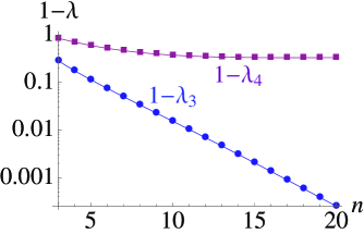
Figure 1: (Color online) The non-trivial eigenvalues $\lambda_{3}$ and $\lambda_{4}$ of the transition matrix $W$.

This analysis also suggests when the mean-field theory breaks down — the theory is not applicable once the third eigen-component significantly decays at around $t_{3}$. That is, after an exponential time of $\exp(0.41n)$, the distribution of the overlap becomes the linear combination of $f_{1}(q)$ and $f_{2}(q)$, i.e., every state becomes either the same or the sign-flip of the others. However, this never happens in a real system.

In the remaining part of this section, we characterize in more detail the quasi-stationary state in large $n$ limit, from which we extract the structure of attractors.

We first introduce an auxiliary notation

$$\alpha_{t+l,t}(q)\equiv\frac{1}{n}\ln P_{t+l,t}(q),$$ (8)

where $\int\exp(n\alpha_{t+l,t}(q))dq=1$ according to the normalization constraint. With this notation, we can express the dynamics of Eq. (4) by

$$\alpha_{t+l+1,t+1}(q) = \frac{1}{n}\ln\int W(q|q^{\prime})P_{t+l,t}(q^{\prime})dq^{\prime}$$ (9)

$$\approx H(q)+\max_{q^{\prime}}\left[\frac{1+q}{2}\ln\frac{1+\varphi(q^{\prime})}{2}+\frac{1-q}{2}\ln\frac{1-\varphi(q^{\prime})}{2}+\alpha_{t+l,t}(q^{\prime})\right],$$

where the Laplace’s method was applied in the second line assuming large $n$. Note that, in the above expression, the maximizer $q^{\prime}$ of the second term is a function of $q$. In particular, the well-defined asymptotic solution of Eq. (9), i.e.,

$$\alpha_{*}(q)=H(q)+\max_{q^{\prime}}\left[\frac{1+q}{2}\ln\frac{1+\varphi(q^{\prime})}{2}+\frac{1-q}{2}\ln\frac{1-\varphi(q^{\prime})}{2}+\alpha_{*}(q^{\prime})\right],$$ (10)

with finite $\alpha_{*}(q)$ self-consistently provides the quasi-stationary state. Note that Eq. (10) permits arbitrary discontinuity of $\alpha_{*}(q)$ at $q=\pm 1$, reflecting that $q=\pm 1$ is the sink of the Markovian process. However, in the following analysis, we assume continuous $\alpha_{*}(q)$.

Next, we define index $\beta_{t+l,t}(q_{ts})\equiv\frac{1}{n}\ln\mbox{Prob}(q_{t+l,t}|q_{t+l+1,t+1}=1)$ that characterizes the probability that two states $\boldsymbol{\sigma}(t+l)$ and $\boldsymbol{\sigma}(t)$ have overlap $q_{t+l,t}$ before converging in the next step ($q_{t+l+1,t+1}=1$). This index is expressed, using the Bayes theorem, in terms of $\alpha$ by

$$\beta_{t+l,t}(q^{\prime}) = \frac{1}{n}\ln\frac{W(1|q^{\prime})P_{t+l,t}(q^{\prime})}{P_{t+l+1,t+1}(1)}$$ (11)

$$= \ln\frac{1+\varphi(q^{\prime})}{2}+\alpha_{t+l,t}(q^{\prime})-\alpha_{t+l+1,t+1}(1).$$

This means that, for large $n$, most of the trajectories that lead to state concentration had an overlap specified by the peak location of $\beta_{t+l,t}$, i.e., $\arg\max_{q^{\prime}}\beta_{t+l,t}(q^{\prime})$, in the previous step.

(a)	(b)

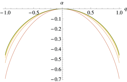
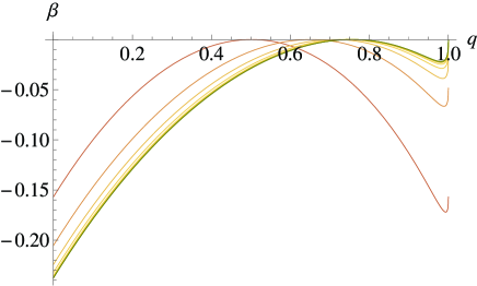
Figure 2: (Color online) The Markovian dynamics of $\alpha_{t+l,t}$ and $\beta_{t+l,t}$ in time. (a) The index $\alpha_{t+l,t}$ characterizes the dynamics of distribution $P(q_{t+l,t})$. The line color changes from the lowest curve (the orange curve at $t=0$, i.e., $\alpha_{l,0}$ or $\beta_{l,0}$) to the yellow, and finally to the gray (the top curve at $t=10$, i.e., $\alpha_{l+10,10}$ or $\beta_{l+10,10}$). (b) The index $\beta_{t+l,l}$ characterizes the dynamics of distribution $P(q_{t+l,t}|q_{t+l+1,t+1}=1)$. The result indicates that states concentrate mainly from $q\approx 0.5$ at the beginning but concentrate equally from $q\approx 0.75$ and $q=1$ at the quasi-stationary state. We used $\alpha_{l,0}(q)=H(q)-\ln 2$ as the initial condition assuming no correlations at starting points. The results hold for any $l\geq 1$.

In the case of randomly connected neural networks studied here, $\beta_{t+l,t}(q)$ has two peaks. As shown in Fig. 2 (b), one peak is located at $q=1$ reflecting the monotonic increase in $\ln\frac{1+\varphi(q)}{2}$ toward $q=1$ and the other peak is located at $q<1$ reflecting the peak of $\alpha_{t+l,t}(q)$ at $q=0$ in Eq. (11). The $q<1$ peak shifts to a larger positive value of $q$ and its amplitude loses the dominance over the $q=1$ peak as $t$ increases because $\alpha_{t+l,t}(q)$ becomes blunt at large $t$ (Fig. 2 (a)). The two peaks become comparable at around $t_{4}$. In finite-size systems, the two peaks become indistinguishable once the difference of the peak values becomes less than $1/n$. The result indicates that states concentrate mainly from $q\approx 0.5$ at the beginning but concentrate equally from $q\approx 0.75$ and $q=1$ at the quasi-stationary state.

These dynamics of the state overlap reflects the specific structure of attractors as we shall show below. In contrast to the above situation, for trivial dynamical systems that converge to a unique fixed-point (e.g., $h_{i}(t+1)=(1+h_{i}(t))/2$), $\beta_{t+l,t}(q)$ has a unique peak, which tends to approach $q=1$ at large $t$, indicating that most states concentrate from nearby locations. On the other hand, in random Boolean networks, states concentrate randomly from any overlap values. Because most states are orthogonal to each other for large $n$, states mainly concentrate from $q\approx 0$ (see Appendix C).

V Statistical properties of attractors

In this section, we analytically describe the statistical properties of attractors for randomly connected neural networks using the state concentration probability Amari et al. (2013). The state concentration probability $p_{t+1,s+1}$ that characterizes the conditional probability of $\boldsymbol{\sigma}(t+1)=\boldsymbol{\sigma}(s+1)$ given that no states up to time $t$ along the trajectory are the same or the sign-flip of the others. Because of the symmetry, $p_{t+1,s+1}$ also characterizes the probability of $\boldsymbol{\sigma}(t+1)=-\boldsymbol{\sigma}(s+1)$ given the same condition. Hence,

$$p_{t+1,s+1} \equiv \mbox{Prob}(q_{t+1,s+1}=\pm 1|\{q_{t^{\prime},s^{\prime}}\neq\pm 1|t^{\prime}\leq t,s^{\prime}<t^{\prime}\}).$$ (12)

This state concentration probability is further approximated under the Markovian approximation of Eq.(4) by

$$p_{t+1,s+1} \approx \int_{q_{ts}\neq\pm 1}W(q_{t+1,s+1}=1|q_{ts})P(q_{ts})dq_{ts}$$ (13)

$$= \exp(n\alpha_{t+1,s+1}(1)),$$

which directly follows from Eq. (9). Note that, based on the consideration of the previous section, we used in the second line that the result is not sensitive to the exclusion of $q^{\prime}=\pm 1$ from the integral for large $n$. This is because the $\max_{q^{\prime}}$ in Eq. (9) is insensitive to its argument at $q^{\prime}=\pm 1$ unless the initial distribution $P_{l,0}(q)$ is sharply peaked at $q=\pm 1$, which is not the case here (c.f. Eq. (6)).

Hence, based on the Markovian property, the probability that the dynamics starting from $\boldsymbol{\sigma}(0)$ comes back for the first time to $\boldsymbol{\sigma}(0)$ after $l$ steps without visiting any sign-flip of previously visited states is described for large $n$ by

$$\tilde{P}(l) \equiv \mbox{Prob}\left(\{q_{1,0}\neq\pm 1\},\{q_{2,s}\neq\pm 1|s=0,1\},\cdots,\{q_{l-1,s}\neq\pm 1|s=0,1,\dots,l-2\},\,q_{l,0}=1\right)$$ (14)

$$= (1-2p_{1,0})\prod_{s=0}^{1}(1-2p_{2,s})\cdots\prod_{s=0}^{l-2}(1-2p_{l-1,s})p_{l,0}$$

$$= p_{l,0}\exp\left(\sum_{t=1}^{l-1}\sum_{s=0}^{t-1}\ln(1-2p_{t,s})\right).$$

Note that, in the second line of Eq. (14), the factor $\prod_{s=0}^{t-1}(1-2p_{t,s})$ describes the probability that the state makes a transition at time $t$ to a state distinct from $\{\pm\boldsymbol{\sigma}(s)|s=0,1,\dots,t-1\}$. The final factor, $p_{l,0}$, describes the probability of coming back to the initial state $\boldsymbol{\sigma}(0)$ after $l$ steps.

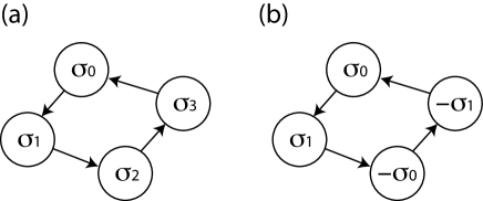
Figure 3: There are two kinds of limit cycles if the cycle length $l$ is even. (a) In the first kind of cycles, the cycle closes without ever visiting the sign-flip of previously visited states. (b) In the second kind of cycles, the state first makes a transition to the sign-flip of the initial state after $l/2$ steps, i.e., $\boldsymbol{\sigma}(l/2)=-\boldsymbol{\sigma}(0)$. If this happens, the cycle must close after $l$ steps.

Altogether, the probability that a certain state, $\boldsymbol{\sigma}(0)$, belongs to a cycle of length $l$ (revisiting $\boldsymbol{\sigma}(0)$ for the first time after $l$ steps) is described for large $n$ by Bastolla and Parisi (1997)

$$P(l) = \left\{\begin{array}[]{cc}\tilde{P}(l),&(\mbox{odd $l$})\\ \tilde{P}(l)+\tilde{P}(l/2).&(\mbox{even $l$})\end{array}\right.$$ (17)

Notably, the probability takes different expressions for odd and even $l$. If $l$ is odd, Eq. (14) directly gives the probability. If $l$ is even, there are two separate kinds of contributions depicted in Fig. 3. The first contribution is from cycles that close without ever visiting the sign-flip of their history. The second contribution is from cycles that involve a transition at step $l/2$ to the sign-flip of their initial state, which then guarantees that the cycle closes in $l$ steps.

The final step is to evaluate the state concentration probability $p_{t,s}$. The initial state concentration probabilities are simply given by

$$p_{l,0}\approx 2^{-n}\equiv p_{\rm init}$$ (18)

for large $n$ and $l$ as discussed in Sec. III. Although this approximation is inaccurate for $l<10$, it becomes accurate for large $n$ over a wide range of $l$ that includes the typical cycle length (Fig. 4).

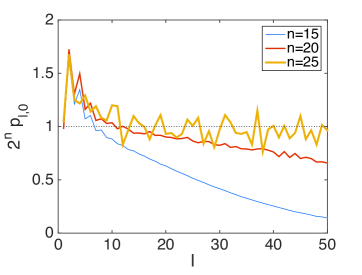
Figure 4: (Color online) Simulation results of the initial state concentration probability $p_{l,0}$ as a function of $l$ when $n$ varies. The results are obtained based on statistics collected from $2\times 10^{9}$ networks. The initial state is always set to $\sigma_{i}(0)=1$ for all $i$ (see Appendix B). The sampling error increases with $n$ because of exponential increase of the state space. Note that $p_{1,0}=2^{-n}$ is an exact result.

On the other hand, the state concentration probability $p_{t+l,t}$ at $t\geq 1$ is computed sequentially by Eqs. (9) and (13). In particular, this probability quickly converges within several steps ($t_{c}\approx 5$; see, Fig. 2 (a)) to the quasi-stationary value of

$$p_{\infty} \equiv \lim_{t\to\infty}p_{t+l,t}=\exp\left(n\alpha(1)\right)$$ (19)

for any $l\geq 1$, where $\alpha(1)=-0.46$ from Eq. (10). That is, the state concentration probability quickly converges in several steps from the initial value of $p_{\rm init}\approx\exp(-0.69n)$ to the asymptotic value $p_{\infty}\approx\exp(-0.46n)$.

Therefore, $\tilde{P}(l)$ of Eq. (14) can be further approximated using $p_{\rm init}$ and $p_{\infty}$ by

$$\tilde{P}(l) = p_{\rm init}\exp\left[\sum_{t=1}^{l-1}\sum_{s=0}^{t-1}\ln(1-2p_{\infty})+O\left(2t_{c}l\frac{p_{\infty}-p_{\rm init}}{1-2p_{\infty}}\right)\right]$$ (20)

$$\approx p_{\rm init}\exp\left[\frac{l^{2}}{2}\ln(1-2p_{\infty})\right]$$

$$= p_{\rm init}\exp\left(-\frac{l^{2}}{\tau^{2}}\right),$$

where $\tau\equiv\sqrt{-2/\ln(1-2p_{\infty})}$ is the characteristic cycle length that grows exponentially with the system size, consistent with the numerical observations Nützel (1991). Note that, in the first line of Eq. (20), we used the relationship that $|p_{\infty}-p_{ts}|\leq|p_{\infty}-p_{\rm init}|$ (for any $t$ and $s$; see, Fig. 2) to upper-bound the deviation of $p_{ts}$ from $p_{\infty}$. To make the contribution of the $O\left(2t_{c}l\frac{p_{\infty}-p_{\rm init}}{1-2p_{\infty}}\right)$ negligible, the approximation in the second line assumes

$$4t_{c}\frac{p_{\infty}-p_{\rm init}}{-(1-2p_{\infty})\ln(1-2p_{\infty})}\ll l\;\;{\rm and}\;\;l\ll\frac{1-2p_{\infty}}{2t_{c}(p_{\infty}-p_{\rm init})}.$$ (21)

The first condition in Eq. (21) requires that $-\frac{l^{2}}{2}\ln(1-2p_{\infty})\gg 2t_{c}l\frac{p_{\infty}-p_{\rm init}}{1-2p_{\infty}}$, while the second condition ensures that $2t_{c}l\frac{p_{\infty}-p_{\rm init}}{1-2p_{\infty}}\ll 1$. The range of $l$ specified by Eq. (21) is roughly $10\ll l\ll\exp(0.46n)/(2t_{c})$ at $n>10$. Hence, the characteristic cycle length $\tau\approx\exp(0.23n)$ is well within this range. Incidentally, $\tau$ is known to also characterize the typical transient time scale to enter a limit cycle Bastolla and Parisi (1997).

(a)	(b)

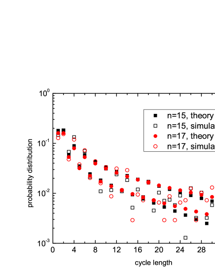
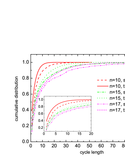
Figure 5: (Color online) (a) Probability distribution of cycle lengths. (b) Cumulative distribution of cycle lengths. The numerical data is obtained from $1000$ samples for $n=10$, $500$ samples for $n=15$, and $200$ samples for $n=17$. The inset shows an enlarged view at small cycle length.

(a)	(b)

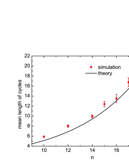
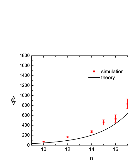
Figure 6: (Color online) The first (mean) and second moment of the cycle length distribution. Theoretical predictions and numerical simulations are compared. The results are averaged over many random realizations of the networks (from $1000$ samples for $n=10$ to $100$ samples for $n=18$).

The probability of observing a cycle of length $l$ is given by $P(l)/(lZ)$ with a normalization constant $Z\equiv\sum_{l=1}^{2^{n}}P(l)/l$. In this expression, the probability, $P(l)$, of a state belonging to a cycle of length $l$ should be divided by $l$ to provide the cycle length probability since all states within a cycle share the same cycle length. Note that the normalization constant $Z$ represents the probability of a state belonging to a cycle (attractor). Figure 5 (a) shows the comparison of numerically obtained cycle length probability with its theoretical estimate. Numerical details to collect the statistics of the attractors are given in the Appendix D. The theory nicely captures this probability at around the characteristic cycle length, including the difference in probability for odd and even cycle lengths, as $n$ becomes large. However, the deviation is large for non-typical $l$ in finite networks. The cumulative distribution of cycle length is similarly obtained by $F(l)\equiv(1/Z)\sum_{l^{\prime}=1}^{l}P(l^{\prime})/l^{\prime}\approx\left(\int_{1}^{l}\tilde{P}(l^{\prime})/l^{\prime}{\rm d}l^{\prime}+\int_{1}^{l/2}\tilde{P}(l^{\prime})/(2l^{\prime}){\rm d}l^{\prime}\right)/Z$ . The comparison of $F(l)$ with the numerical results is shown in Fig. 5 (b). The discrepancy tends to become small for larger $n$ (see the inset of Fig. 5 (b)).

The first moment (mean value) and the second moment of the distribution can be computed analytically as well. Their values are given by:

$$\left<l\right> = \frac{4\sqrt{\pi}\tau\left[1-{\rm erf}(1/\tau)\right]}{3\int^{\infty}_{1/\tau^{2}}\frac{e^{-t}}{t}{\rm d}t},$$ (22)

$$\left<l^{2}\right> = \frac{2\tau^{2}e^{-1/\tau^{2}}}{\int^{\infty}_{1/\tau^{2}}\frac{e^{-t}}{t}{\rm d}t},$$ (23)

where ${\rm erf}(x)=\frac{2}{\sqrt{\pi}}\int_{0}^{x}e^{-t^{2}}{\rm d}t$ and $\int^{\infty}_{1/\tau^{2}}\frac{e^{-t}}{t}{\rm d}t\simeq-\gamma_{{\rm E}}-\alpha(1)n$ in the large $n$ limit, where $\gamma_{\rm E}=0.5772$ is the Euler constant. The theoretical predictions are compared with the numerical results in Fig. 6. The exponential growth of the typical cycle length is verified, which suggests that chaotic attractors exist in the state space of a randomly connected neural network.

(a)	(b)

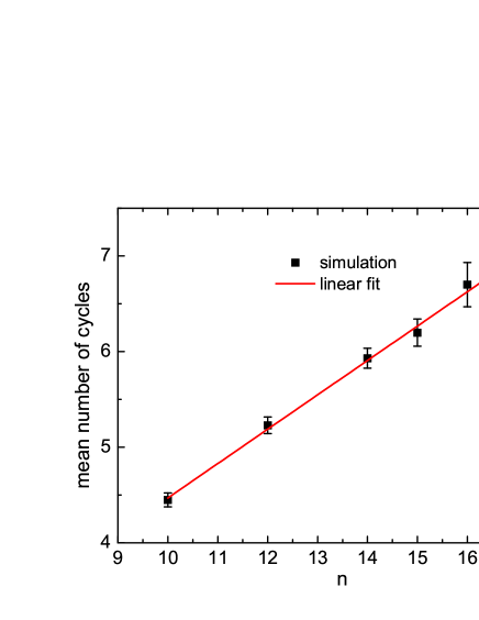
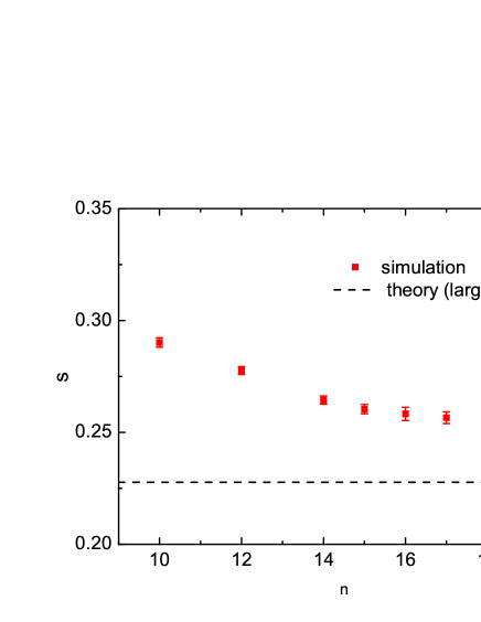
Figure 7: (Color online) (a) Linear dependence of the number of cycles on network size $n$. (b) Entropy density of the attractive states defined by $s=\frac{1}{n}\ln N_{{\rm att}}$. As $n$ increases, the numerical data gets to the theoretical prediction.

Following the same spirit, one can derive the number of attractors as $2^{n}Z\simeq-3\alpha(1)n/4-3\gamma_{\rm E}/4$, from which a linear dependence Gutfreund et al. (1988); Schreckenberg (1992); Bastolla and Parisi (1997) is confirmed (see also Fig. 7 (a), the linear fit gives the slope $0.360\pm 0.010$, compatible with the theoretical value $0.342$). Another interesting quantity is the number of the attractive states $N_{{\rm att}}$ belonging to all cycles (e.g., a cycle of length $l$ has $l$ attractive states), which is expected to grow exponentially with the network size $n$. This quantity is evaluated by our theory as $N_{{\rm att}}=2^{n}\sum_{l=1}^{2^{n}}P(l)$, and can be quantified as the growth rate (entropy density) $s=\lim_{n\rightarrow\infty}\frac{1}{n}\ln N_{{\rm att}}$. In the large $n$ limit, we obtain $s=-\alpha(1)/2$, which is compared with the numerical results at finite $n$. As shown in Fig. 7 (b), as $n$ increases, $s$ decreases, approaching the asymptotic limit $0.2277$.

The deviation at small $n$ (or at $l$ far from the characteristic length, see Fig. 5) comes from three approximations. One is Eq. (18), which becomes invalid at small $l$ where $p_{\rm init}$ also depends on $l$, but Eq. (18) becomes reasonable for large $l$ (as occurs in our case where the typical cycles are long). The second one is Eq. (20). This approximation is valid in the range of $l$ specified by Eq. (21). Note that this condition is consistent with the numerical results shown in Fig. 5. The last approximation is Eq. (4), which breaks down for small $n$ at which two or more time-steps memory should be considered. In the large network size limit, these approximations become exact and the dynamics can be described by a Markovian process in terms of the state overlap. Thus, as we focus on the structure of attractors at a relatively large but finite $n$, these effects are not significant.

VI Conclusion

In this work, we studied the deterministic dynamics of a randomly connected neural network and proposed a simple Markovian stochastic process to describe the evolution of the overlap of two states along the dynamics trajectories. The properties of the state concentration can be studied by a mean field computation, and furthermore, the theoretical cumulative distribution of cycle length is compared with the numerical simulation results. The typical length of cycles is predicted and observed to grow exponentially with the network size. The number of attractive states on all cycles has also an exponential growth with the network size, and its typical value can also be predicted by our theory.

Our theory should have potential to be generalized to treat more complex situations, e.g., couplings between neurons are correlated, where one time-step memory is not enough to describe the dynamics and strong memory effects induced by retarded self-interaction could be incorporated by introducing a back-action field (two time-steps memory) Huang and Kabashima (2014). The current analysis is also restricted to the parallel type of dynamics, whereas, the sequential (asynchronous) dynamics seems to be more natural, and our current method may apply to this type of dynamics, although the computation will become more complicated. However, the statistical properties of attractors would not change qualitatively, as expected from numerical simulations Gutfreund et al. (1988).

Our work is expected to provide insights towards understanding how the neural network processes information and stores temporal sequences Vogels et al. (2005), which will be left for future study.

Appendix A Dynamic functional integral method

We compute the dynamics of the state overlap using the dynamic functional integral (mean-field) method (see Toyoizumi and Abbott (2011) for similar calculations). In this section, we express time indices as lower case characters, e.g., $h_{i}(t)=h_{it}$, and follow the convention that summations are neglected if the same indices appear twice in an expression, e.g., $\sum_{j}J_{ij}\sigma_{jt}=J_{ij}\sigma_{jt}$.

Let us first define the ensemble of state trajectories, $\boldsymbol{h}=\{h_{it}|i=1,\dots,n,\,t=0,1,\dots\}$, averaged over different networks:

$$P(\boldsymbol{h})\equiv\left[\prod_{i,t}\delta\left(h_{it}-J_{ij}\sigma_{jt}\right)\right]_{J},$$ (24)

where $\delta(\cdot)$ is the Dirac delta function and $[\cdot]_{J}$ is the average over the random couplings. In the following, we denote by $\langle\cdot\rangle$ an average with respect to $P(\boldsymbol{h})$.

The joint distribution of the overlap $\boldsymbol{q}=\{q_{ts}\}_{t>s}$ is

$$P(\boldsymbol{q}) \equiv \left\langle\prod_{t>s}\delta\left(q_{ts}-\frac{1}{n}\sigma_{jt}\sigma_{js}\right)\right\rangle$$

$$= \int\left(\prod_{i,t}dh_{it}\right)\left[\prod_{i,t}\delta(h_{it}-J_{ij}\sigma_{jt})\right]_{J}\prod_{t>s}\delta\left(q_{ts}-\frac{1}{n}\sigma_{jt}\sigma_{js}\right)$$

$$= \int\left(\prod_{i,t}\frac{dh_{it}d\hat{h}_{it}}{2\pi}\right)\left[\exp\left(\mathrm{i}\hat{h}_{it}h_{it}-\mathrm{i}\hat{h}_{it}J_{ij}\sigma_{jt}\right)\right]_{J}\prod_{t>s}\delta\left(q_{ts}-\frac{1}{n}\sigma_{jt}\sigma_{js}\right)$$

$$= \int\left(\prod_{i,t}\frac{dh_{it}d\hat{h}_{it}}{2\pi}\right)\exp\left(\mathrm{i}\hat{h}_{it}h_{it}-\frac{1}{2n}\hat{h}_{it}\hat{h}_{is}\sigma_{jt}\sigma_{js}\right)\prod_{t>s}\delta\left(q_{ts}-\frac{1}{n}\sigma_{jt}\sigma_{js}\right)$$

$$= \int\left(\prod_{i,t}\frac{dh_{it}d\hat{h}_{it}}{2\pi}\right)\exp\left(\mathrm{i}\hat{h}_{it}h_{it}-\frac{1}{2}q_{ts}\hat{h}_{it}\hat{h}_{is}\right)\prod_{t>s}\delta\left(q_{ts}-\frac{1}{n}\sigma_{jt}\sigma_{js}\right)$$

$$= \int\left(\prod_{t>s}\frac{nd\hat{q}_{ts}}{2\pi}\right)\int\left(\prod_{i,t}\frac{dh_{it}d\hat{h}_{it}}{2\pi}\right)\exp\left(n\mathrm{i}\hat{q}_{ts}q_{ts}-\mathrm{i}\hat{q}_{ts}\sigma_{jt}\sigma_{js}+\mathrm{i}\hat{h}_{it}h_{it}-\frac{1}{2}q_{ts}\hat{h}_{it}\hat{h}_{is}\right)$$

$$= \int\left(\prod_{t>s}\frac{nd\hat{q}_{ts}}{2\pi}\right)\exp(-nf(\boldsymbol{q},\hat{\boldsymbol{q}})),$$

where we have defined the action

$$f(\boldsymbol{q},\hat{\boldsymbol{q}})\equiv-\mathrm{i}\hat{q}_{ts}q_{ts}-\ln\int dH\exp\mathcal{L},$$ (26)

$$\mathcal{L}\equiv\mathrm{i}\hat{h}_{t}h_{t}-\frac{1}{2}q_{ts}\hat{h}_{t}\hat{h}_{s}-\mathrm{i}\hat{q}_{ts}\sigma_{t}\sigma_{s},$$

and $dH\equiv\prod_{t}(dh_{t}d\hat{h}_{t})/(2\pi)$. In the derivation, we have used the Fourier transformation of the delta function $\delta(x)=\int d\hat{x}/(2\pi)\exp(\mathrm{i}\hat{x}x)$ for each delta function in Eq. (A), and we have taken the average over the independent Gaussian variables $\{J_{ij}\}$ of mean 0 and variance $1/n$. For large $n$, the distribution of Eq. (A) is well approximated by a Gaussian distribution, where the peak is specified by the saddle-point equations:

$$0 = \frac{\partial f}{\partial q_{ts}}=-\mathrm{i}\hat{q}_{ts}+\frac{1}{2}\langle\hat{h}_{t}\hat{h}_{s}\rangle_{\mathcal{L}},$$ (27)

$$0 = \frac{\partial f}{\partial\mathrm{i}\hat{q}_{ts}}=-q_{ts}+\langle\sigma_{t}\sigma_{s}\rangle_{\mathcal{L}},$$

with average $\langle\cdot\rangle_{\mathcal{L}}\equiv(\int\cdot e^{\mathcal{L}}dH)/(\int e^{\mathcal{L}}dH)$. We can easily see that $\hat{\boldsymbol{q}}=0$ is a solution of Eq. (27) Toyoizumi and Abbott (2011). Hence, if $\hat{\boldsymbol{q}}=0$, the average $\langle\cdot\rangle_{\mathcal{L}_{0}}\equiv\langle\cdot\rangle_{\mathcal{L}}|_{\hat{\boldsymbol{q}}=0}$ is an average over Gaussian $\boldsymbol{h}$ of mean $\langle h_{t}\rangle_{\mathcal{L}_{0}}=0$ and covariance $\langle h_{t}h_{s}\rangle_{\mathcal{L}_{0}}=q_{ts}$, which simplifies the saddle-point equation of Eq. (27) in terms of a closed-form expression of $\boldsymbol{q}$ by

$$q_{t+1,s+1} = \langle\sigma_{t+1}\sigma_{s+1}\rangle_{\mathcal{L}_{0}}$$

$$= \iint DxDy\,\mbox{sgn}(x)\mbox{sgn}\left(q_{ts}x+\sqrt{1-q_{ts}^{2}}y\right)$$

$$= \varphi(q_{ts}),$$

with $\varphi(q)\equiv(2/\pi)\arcsin(q)$ and a Gaussian measure $Dx\equiv\exp(-x^{2}/2)/\sqrt{2\pi}$. Note that $|\varphi(q)|\leq|q|$ and the equality holds only at $q=0$ and $q=\pm 1$. Hence, unless $q=1$ initially, the overlap rapidly converges in a few steps to zero in the $n\to\infty$ limit.

The order parameters fluctuate around the saddle-point solution of Eq. (A) for finite $n$. This fluctuation of $\boldsymbol{q}$ and $\hat{\boldsymbol{q}}$ is characterized to the leading order by the Hessian matrix of $f$, i.e.,

$$A_{ts,t^{\prime}s^{\prime}} \equiv \frac{\partial^{2}f}{\partial q_{ts}\partial q_{t^{\prime}s^{\prime}}}=\frac{1}{2}\frac{\partial\langle\hat{h}_{t^{\prime}}\hat{h}_{s^{\prime}}\rangle_{\mathcal{L}_{0}}}{\partial q_{ts}},$$ (29)

$$B_{ts,t^{\prime}s^{\prime}} \equiv \frac{\partial^{2}f}{\partial q_{ts}\partial\hat{q}_{t^{\prime}s^{\prime}}}=-\mathrm{i}\delta_{t,t^{\prime}}\delta_{s,s^{\prime}}+\mathrm{i}\frac{\partial\langle\sigma_{t^{\prime}}\sigma_{s^{\prime}}\rangle_{\mathcal{L}_{0}}}{\partial q_{ts}},$$

$$C_{ts,t^{\prime}s^{\prime}} \equiv \frac{\partial^{2}f}{\partial\hat{q}_{ts}\partial\hat{q}_{t^{\prime}s^{\prime}}}=\langle\sigma_{t}\sigma_{s}\sigma_{t^{\prime}}\sigma_{s^{\prime}}\rangle_{\mathcal{L}_{0}}-\langle\sigma_{t}\sigma_{s}\rangle_{\mathcal{L}_{0}}\langle\sigma_{t^{\prime}}\sigma_{s^{\prime}}\rangle_{\mathcal{L}_{0}},$$

for $t>s$ and $t^{\prime}>s^{\prime}$, where the Hessian matrix is evaluated at the saddle-point solution of the order parameters, i.e., $\hat{\boldsymbol{q}}=0$ and the solution of Eq. (A).

In the current setup, the Hessian matrix is simply given by

$$A_{ts,t^{\prime}s^{\prime}} = 0,$$ (30)

$$B_{ts,t^{\prime}s^{\prime}} = -\mathrm{i}\delta_{t,t^{\prime}}\delta_{s,s^{\prime}}+\mathrm{i}\varphi^{\prime}(q_{ts})\delta_{t^{\prime},t+1}\delta_{s^{\prime},s+1},$$

$$C_{ts,t^{\prime}s^{\prime}} = \delta_{t,t^{\prime}}\delta_{s,s^{\prime}}+O(q^{2}),$$

for $t>s$ and $t^{\prime}>s^{\prime}$, where $\varphi^{\prime}(q)\equiv d\varphi(q)/dq$. Note that the $O(q^{2})$ contribution in $C_{ts,t^{\prime}s^{\prime}}$ can be more explicitly estimated, for example by applying Plackett’s approximation Bacon (1963). Here, we would like to evaluate the ($n$ multiplied) covariance of the overlap parameter, $\tilde{A}_{ts,t^{\prime}s^{\prime}}\equiv n\mbox{Cov}[q_{ts},q_{t^{\prime}s^{\prime}}]$. By applying the matrix inversion lemma, we find that its inverse is

$$\tilde{A}^{-1}=A-BC^{-1}B^{T}=(\mathrm{i}B)(\mathrm{i}B)^{T}+O(q^{2}).$$ (31)

This relation indicates that for small $\boldsymbol{q}$ the linear combination,

$${\boldsymbol{\eta}} \equiv \sqrt{n}(\mathrm{i}B)^{T}{\boldsymbol{\delta q}},$$ (32)

of the fluctuation of the overlap parameter, ${\boldsymbol{\delta q}}$, is white Gaussian random variables. To see this, one can apply the transformation of variables and find that

$$P({\boldsymbol{\eta}}) = \int\delta\left({\boldsymbol{\eta}}-\sqrt{n}(\mathrm{i}B)^{T}{\boldsymbol{\delta q}}\right)\exp\left(-\frac{n}{2}{\boldsymbol{\delta q}}^{T}\tilde{A}^{-1}{\boldsymbol{\delta q}}\right)d{\boldsymbol{\delta\boldsymbol{q}}}$$ (33)

$$\sim \exp\left(-\frac{1}{2}{\boldsymbol{\eta}}^{T}{\boldsymbol{\eta}}\right).$$

Thus, Eq. (32) indicates that the finite-size fluctuations of the order parameter are described by

$$\frac{1}{\sqrt{n}}\eta_{ts} = \left[\delta_{t^{\prime},t}\delta_{s^{\prime},s}-\varphi^{\prime}(q_{t^{\prime}s^{\prime}})\delta_{t,t^{\prime}+1}\delta_{s,s^{\prime}+1}\right]\delta q_{t^{\prime}s^{\prime}}$$ (34)

$$= \delta q_{ts}-\varphi^{\prime}(q_{t-1,s-1})\delta q_{t-1,s-1}.$$

Altogether, summarizing that $q_{ts}=\varphi(q_{t-1,s-1})$ in the $n\to\infty$ limit and that the finite-size correction is described by Eq. (34), we obtained, for finite $n$,

$$q_{ts}=\varphi(q_{t-1,s-1})+\frac{1}{\sqrt{n}}\eta_{ts}+O(q^{2}),$$ (35)

which is a simple Markovian process that involves white Gaussian noise of variance $1/n$.

Recalling the definition of the overlap parameter, $q_{t+1,s+1}=\mbox{sgn}(h_{it})\mbox{sgn}(h_{is})/n$, and that $h_{i}$ with different $i$ tend to become independent in the $n\to\infty$ limit, we know that the overlap parameter must be distributed approximately according to a binomial distribution. Extrapolating this observation, the result of Eq. (35) is consistent with the Markovian dynamics of

$$P(q_{t+1,s+1})=\int W(q_{t+1,s+1}|q_{ts})P(q_{ts})dq_{ts}$$ (36)

with the binomial transition probability

$$W\left(\left.q_{t+1,s+1}=\frac{2m-n}{n}\right|q_{ts}\right)=\binom{n}{m}\left(\frac{1+\varphi(q_{ts})}{2}\right)^{m}\left(\frac{1-\varphi(q_{ts})}{2}\right)^{n-m},$$ (37)

where $m$ indicates the number of units taking the same state at time $t+1$ and $s+1$.

In summary, this result shows that the Markovian dynamics of Eq. (36) provides a good approximation of the dynamics of the overlap parameter once $O(q^{2})$ terms become negligible near the stationary state.

Appendix B The dynamics of the state overlap does not depend on the initial state $\sigma(0)$

A specific choice of the initial state $\boldsymbol{\sigma}(0)$ is not important to study dynamics of the state overlap for random ensemble of networks as long as $\boldsymbol{\sigma}(0)$ is selected independently of the network connections $\{J_{ij}\}$. Without losing generality, we can set $\sigma_{i}(0)=1$ for all $i$.

To see this point, we consider a simple transformation of variables,

$$\tilde{\sigma}_{i}(t)=\sigma_{i}(t)\sigma_{i}(0).$$ (38)

The state overlap is also described in terms of these transformed variables by $q_{ts}=(1/n)\sum_{i}\tilde{\sigma}_{i}(t)\tilde{\sigma}_{i}(s)$ and the initial state is given by $\tilde{\sigma}_{i}(0)=1$ for all $i$.

These transformed variables follow the same update rule as the original one,

$$\tilde{\sigma}_{i}(t+1)=\mbox{sgn}\left(\sum_{j}\tilde{J}_{ij}\tilde{\sigma}_{j}(t)\right),$$ (39)

except that the coupling matrix is given by $\tilde{J}_{ij}=\sigma_{i}(0)J_{ij}\sigma_{j}(0)$ instead of $J_{ij}$. Notably, the distribution of $\{\tilde{J}_{ij}\}$ is the same as that of $\{J_{ij}\}$ as long as $\boldsymbol{\sigma}(0)$ is chosen independently of $\{J_{ij}\}$. Therefore, to study the dynamics of the state overlap, we can alternatively study the dynamics of these transformed variables with the initial condition $\{\tilde{\sigma}_{i}(0)=1|i=1,2,\dots,n\}$.

Appendix C The dynamics of the state overlap in random Boolean networks

The dynamics of the state overlap in random Boolean networks is described by Eq. (9) with $\varphi_{BN}(q)=\delta_{q,1}$, which is simply

$$\alpha_{t+1,s+1}(q) = \left\{\begin{array}[]{ll}H(q)-\ln 2+\alpha_{ts}^{*},&(q\neq 1)\\ \max\left\{\alpha_{ts}(1),-\ln 2+\alpha_{ts}^{*}\right\},&(q=1)\end{array}\right.$$ (42)

where $\alpha_{ts}^{*}\equiv\max_{q^{\prime}\neq 1}\alpha_{ts}(q^{\prime})$. Let us assume that there is no perfect overlap of states initially, i.e., $\mbox{Prob}(q_{l,0}=1)=0$. This means that $\alpha_{l,0}(1)<-\ln 2+\alpha_{l,0}^{*}$ and $\lim_{n\to\infty}\alpha_{l,0}^{*}=0$, because the initial overlap distribution $P_{l,0}(q)=\exp(n\alpha_{l,0}(q))$ must be normalized. Thus, the dynamics of Eq. (42) converges in one step to a stationary solution

$$\alpha(q)=H(q)-\ln 2.$$ (43)

Moreover, we have from Eq. (11)

$$\beta(q^{\prime}) = \ln\frac{1+\varphi_{BN}(q^{\prime})}{2}+H(q^{\prime})$$ (44)

$$= \left\{\begin{array}[]{ll}H(q^{\prime})-\ln 2,&(q^{\prime}\neq 1)\\ 0.&(q^{\prime}=1)\end{array}\right.$$ (47)

This indicates that states mainly concentrate from $q=0$ if they do not already concentrate.

This analysis also provides important information about the eigenvalues of the transition matrix $W$ at the large network size limit. The first eigenvalue is trivial, $\lambda_{1}=1$, with the eigenfunction $f_{1}(q)=\delta_{q,1}$, indicating that states never separate once they concentrate. The second eigenvalue, $\lambda_{2}\approx 1$, is a non-trivial one that corresponds to the quasi-stationary state with the eigenfunction $f_{2}(q)=\exp(n\alpha(q))$, where $\alpha(q)$ is given by Eq. (43). The other eigenvalues $\lambda_{k}$ for $k\geq 3$ are all zero because the distribution of the overlap converges in a single step to the quasi-stationary state. Furthermore, the fact that state concentration happens with probability $2^{-n}$ at each time step suggests that $\lambda_{2}=1-2^{-n}$.

Appendix D Simulation details of the dynamics

The total number of states is $2^{n}$. They form a state set called $\mathcal{S}$. We also denote a path set $\mathcal{P}$ recording the states on a dynamics trajectory. Only the state index is stored in both sets.

Step 1.

Choose the first state $\boldsymbol{\sigma}^{1}$ in $\mathcal{S}$ as a starting point for the parallel dynamics, and remove this state from $\mathcal{S}$ at the same time.

Step 2.

$\boldsymbol{\sigma}^{1}$ evolves to $\boldsymbol{\sigma}^{\prime}$ by one step of the parallel dynamics (all neurons’ states are updated for one time).

Step 2.1.

If $\boldsymbol{\sigma}^{\prime}\in\mathcal{S}$, remove it from $\mathcal{S}$, put the index of $\boldsymbol{\sigma}^{\prime}$ into $\mathcal{P}$, and continue to perform the parallel dynamics, i.e., let $\boldsymbol{\sigma}^{1}=\boldsymbol{\sigma}^{\prime}$, then go to Step 2;

Step 2.2

Otherwise, compare $\boldsymbol{\sigma}^{\prime}$ with the one in the set $\mathcal{P}$ and if they coincide with each other, a new cycle is identified and the length is recorded at the same time, then go to Step 3; otherwise, no new cycle is found and go to Step 3.

Step 3.

Go to Step 1 until the set $\mathcal{S}$ becomes empty.

References

- Ko et al. (2011) H. Ko, S. B. Hofer, B. Pichler, K. A. Buchanan, P. J. Sjöström, and T. D. Mrsic-Flogel, Nature 473, 87 (2011).
- Rajan et al. (2010) K. Rajan, L. F. Abbott, and H. Sompolinsky, Phys. Rev. E 82, 011903 (2010).
- Sompolinsky et al. (1988) H. Sompolinsky, A. Crisanti, and H. J. Sommers, Phys. Rev. Lett. 61, 259 (1988).
- van Vreeswijk and Sompolinsky (1996) C. van Vreeswijk and H. Sompolinsky, Science 274, 1724 (1996).
- Toyoizumi and Abbott (2011) T. Toyoizumi and L. F. Abbott, Phys. Rev. E 84, 051908 (2011).
- Ostojic (2014) S. Ostojic, Nature Neuroscience 17, 594 (2014).
- Aljadeff et al. (2014) J. Aljadeff, M. Stern, and T. O. Sharpee, ArXiv e-prints (2014), eprint 1407.2297.
- Sussillo and Abbott (2009) D. Sussillo and L. Abbott, Neuron 63, 544 (2009).
- Laje and Buonomano (2013) R. Laje and D. V. Buonomano, Nature Neuroscience 16, 925 (2013).
- Parisi (1986) G. Parisi, J. Phys. A: Math. Gen. 19, L675 (1986).
- Gardner et al. (1987) E. Gardner, B. Derrida, and P. Mottishaw, J. Physique 48, 741 (1987).
- Gutfreund et al. (1988) H. Gutfreund, J. D. Reger, and A. P. Young, J. Phys. A: Math. Gen. 21, 2775 (1988).
- Rieger et al. (1989) H. Rieger, M. Schreckenberg, and J. Zittartz, Z. Phys. B 74, 527 (1989).
- Schreckenberg (1992) M. Schreckenberg, Z. Phys. B 86, 453 (1992).
- Crisanti et al. (1993) A. Crisanti, M. Falcioni, and A. Vulpiani, J. Phys. A: Math. Gen. 26, 3441 (1993).
- Bastolla and Parisi (1997) U. Bastolla and G. Parisi, J. Phys. A: Math. Gen. 30, 5613 (1997).
- Amari et al. (2013) S.-i. Amari, H. Ando, T. Toyoizumi, and N. Masuda, Phys. Rev. E 87, 022814 (2013).
- Huang and Kabashima (2014) H. Huang and Y. Kabashima, J. Stat. Mech.: Theory Exp p. P05020 (2014).
- Nützel (1991) K. Nützel, J. Phys. A: Math. Gen. 24, L151 (1991).
- Kauffman (1969a) S. A. Kauffman, J. Theor. Biol. 22, 437 (1969a).
- Kauffman (1969b) S. A. Kauffman, Nature 224, 177 (1969b).
- Derrida and Pomeau (1986) B. Derrida and Y. Pomeau, Europhys. Lett 1, 45 (1986).
- Derrida and Stauffer (1986) B. Derrida and D. Stauffer, Europhys. Lett. 2, 739 (1986).
- Derrida (1987) B. Derrida, J. Phys. A 20, L721 (1987).
- Amari (1974) S.-i. Amari, Kybernetik 14, 201 (1974).
- Kürten (1988) K. E. Kürten, Physics Letters A 129, 157 (1988).
- Gallager (2014) R. G. Gallager, Stochastic Processes: Theory for Applications (Cambridge University Press, Cambridge, UK, 2014).
- Bacon (1963) R. H. Bacon, Ann. Math. Statist. 34, 191 (1963).
- Vogels et al. (2005) T. P. Vogels, K. Rajan, and L. F. Abbott, Annu. Rev. Neurosci 28, 357 (2005).