Reduced-rank spatio-temporal modeling of air pollution concentrations in the Multi-Ethnic Study of Atherosclerosis and Air Pollution

Abstract

There is growing evidence in the epidemiologic literature of the relationship between air pollution and adverse health outcomes. Prediction of individual air pollution exposure in the Environmental Protection Agency (EPA) funded Multi-Ethnic Study of Atheroscelerosis and Air Pollution (MESA Air) study relies on a flexible spatio-temporal prediction model that integrates land-use regression with kriging to account for spatial dependence in pollutant concentrations. Temporal variability is captured using temporal trends estimated via modified singular value decomposition and temporally varying spatial residuals. This model utilizes monitoring data from existing regulatory networks and supplementary MESA Air monitoring data to predict concentrations for individual cohort members.

In general, spatio-temporal models are limited in their efficacy for large data sets due to computational intractability. We develop reduced-rank versions of the MESA Air spatio-temporal model. To do so, we apply low-rank kriging to account for spatial variation in the mean process and discuss the limitations of this approach. As an alternative, we represent spatial variation using thin plate regression splines. We compare the performance of the outlined models using EPA and MESA Air monitoring data for predicting concentrations of oxides of nitrogen (NO_x)—a pollutant of primary interest in MESA Air—in the Los Angeles metropolitan area via cross-validated $R^{2}$.

Our findings suggest that use of reduced-rank models can improve computational efficiency in certain cases. Low-rank kriging and thin plate regression splines were competitive across the formulations considered, although TPRS appeared to be more robust in some settings.

FLA

, , , , and T1Supported in part by Grants T32ES015459 and K24ES013195 from the National Institute of Environmental Health Sciences of the National Institutes of Health (NIH). Additional support was provided by the U.S. Environmental Protection Agency (EPA), Assistance Agreement RD-83479601-0 (Clean Air Research Centers) and CR-834077101-0. This publication was developed under a STAR research assistance agreement, No. RD831697, awarded by the U.S Environmental Protection Agency.

1 Introduction

There is growing evidence in the epidemiologic literature of the relationship between air pollution and adverse health outcomes. Early findings were based on somewhat crude regional, and possibly temporally specific, assignment of exposures [Dockery et al. (1993), Pope et al. (2002), Samet et al. (2000)]. Yet, methods for assigning individual exposure to cohort study participants have become much more sophisticated. Recent studies have assigned individual exposure using the value measured at the nearest monitoring location [Miller et al. (2007), Ritz, Wilhelm and Zhao (2006)]; using “land use regression” estimates based on spatially distributed or Geographic Information Systems (GIS) based covariates [Brauer et al. (2003), Hoek et al. (2008), Jerrett et al. (2005a)]; and by interpolation with geostatistical methods such as kriging and semi-parametric smoothing [Jerrett et al. (2005b), Künzli et al. (2005), Paciorek et al. (2009)].

Motivated by the Multi-Ethnic Study of Atheroscelerosis and Air Pollution (MESA Air) study [Kaufman et al. (2012)], Szpiro et al. (2010), Sampson et al. (2011) and Lindström et al. (2013) developed a flexible spatio-temporal prediction model based on monitoring data from existing regulatory networks as well as supplementary MESA Air monitoring data to predict concentrations for individual MESA cohort members. This work integrates land-use regression with kriging to account for spatial dependence in pollutant concentrations. Temporal variability is captured using temporal trends estimated via sparse singular value decomposition and temporally varying spatial residuals [Fuentes, Guttorp and Sampson (2006), Sampson et al. (2011), Szpiro et al. (2010)].

In general, spatio-temporal models are limited in their efficacy for large data sets due to computational intractability. For example, in the purely spatial setting, computation typically is of the order $\mathcal{O}(n^{3})$, where $n$ is the number of spatial locations. The computational effort for log-likelihood evaluation of the MESA Air spatio-temporal model typically grows at least as fast, but slower than $\mathcal{O}(N^{3})$, where $N$ is the total number of spatio-temporal observations [Lindström et al. (2013)]. Methods for reducing the computational burden in spatio-temporal models are becoming more common in the spatial statistics literature. Several authors have proposed dynamic frameworks for modeling residual spatial and temporal dependence, although these approaches continue to suffer from computational intractability [Gelfand, Banerjee and Gamerman (2005), Stroud, Müller and Sansó (2001)]. In the large spatial data context, approximate likelihood and sampling-based approaches have been proposed to reduce computational burden [Fuentes (2007), Pace and LeSage (2009)]. An alternative to approximate methods involves reducing the spatial process to a $K$-dimensional subspace ($K\ll n$) in order to increase computational efficiency [Banerjee et al. (2008), Crainiceanu, Diggle and Rowlingson (2008), Kammann and Wand (2003), Nychka and Saltzman (1998), Stein (2007, 2008)]. These so-called “low-rank” or “reduced-rank” approaches can reduce computation to $\mathcal{O}(K^{3})$.

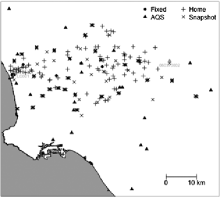
Figure 1: Map of AQS and MESA Air monitoring locations in Los Angeles, California. “Home outdoor” monitors have been jittered for participant confidentiality.

In the current work, we develop reduced-rank versions of the spatio-temporal model outlined in Lindström et al. (2013), Szpiro et al. (2010). Specifically, we apply the approach proposed by Kammann and Wand (2003) to achieve low-rank kriging to account for spatial variation in the mean process and spatially varying temporal trends. We discuss the limitations of this approach and, as an alternative, represent spatial variation using thin plate regression splines [Wood (2003)]. We compare the performance of the outlined models using Environmental Protection Agency (EPA) and MESA Air monitoring data for predicting oxides of nitrogen (NO_x) concentrations in the Los Angeles metropolitan area.

2 Description of data

2.1 Air Quality System (AQS)

The national AQS network of regulatory monitors, managed by the EPA, reports concentrations of a wide variety of air pollutant concentrations on an ongoing basis, most typically hourly averages. For this study, we include NO_x measurements from 21 AQS monitors in the Los Angeles area, one of six metropolitan areas where MESA Air cohort members live. Monitor locations are shown in Figure 1 (left). As MESA Air supplementary monitoring is done at the 2-week average scale, we aggregate AQS monitoring data to 2-week averages. Due to skew in the data, all 2-week averages are log transformed.

2.2 MESA Air

As part of the MESA Air project goals to provide high quality individual exposure prediction, additional monitoring data were collected in each of the study’s six geographic regions, including Los Angeles. The goal of the supplementary monitoring was to provide geographically complementary data to the AQS monitoring data and to systematically span the design space based on proximity to traffic. Additionally, supplementary monitoring data included measurements collected at a subset of cohort participant homes. The sampling strategy is described in more detail by Cohen et al. (2009).

The MESA Air supplementary data is comprised of three classes of monitors, which we refer to as “fixed site,” “home outdoor” and “community snapshot.” There are a total of five “fixed sites” included in this study in the Los Angeles area. These “fixed-sites” began measuring 2-week average concentrations in November of 2005, for a total of 426 measurements by June 1, 2009. A total of 84 “home outdoor” locations were included in this study. These sites were sampled during 2-week periods starting in May of 2006 and ending in February of 2008, for a total of 155 measurements. The sampling plan calls on each home to be measured two times during different seasons. Last, the “community snapshot” sub-campaign consists of 177 sites measured in three rounds of spatially rich sampling during single 2-week periods from July 5, 2006 to January 1, 2007, for a total of 449 measurements. In each round of the “community snapshot” monitoring, most monitors were clustered in groups of six, with three on each side of a major roadway at distances of about 50, 100 and 300 meters, and locations were chosen to span the domain of various land-use categories and to cover a wide geographic region. All MESA Air monitoring locations as of June 1, 2009 are displayed in Figure 1. Likewise, temporal coverage and sampling frequency during the study period for each monitoring location and type is depicted in Figure 2. Table 1 provides summary statistics on the native and log-scales for both EPA and MESA Air data.

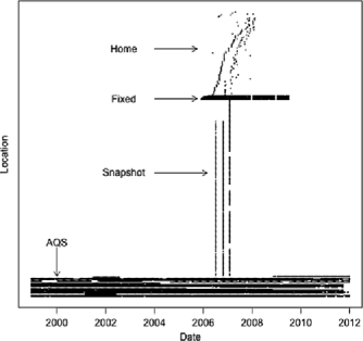
Figure 2: Schematic of sampling schedule for AQS and MESA Air monitors between 1999 and 2012. Each point represents a two-week sampling period.

= $\mathbf{NO}_{\bolds{x}}$ ppb $\operatorname{\mathbf{log}}\textbf{(}\mathbf{NO}_{\bolds{x}}$ ppb) Type of site Mean SD Mean SD AQS/fixed site    2-wk 53.30 40.10 3.72 0.75    LTA 45.35 17.27 3.74 0.39 Community snapshot    2006-07-05 (summer) 34.24 11.49 3.47 0.39    2006-10-25 (fall) 75.09 23.47 4.27 0.32    2007-01-31 (winter) 95.29 26.99 4.51 0.30 Home outdoor 45.65 28.30 3.63 0.64

Table 1: Summary of statistics of NO_x monitoring data at EPA AQS and MESA Air supplementary monitoring sites

2.3 GIS

In addition to the monitoring data, spatial prediction at locations where there are no measurements rely heavily on GIS-based covariates and so-called “land-use regression” techniques [Jerrett et al. (2005a)]. In this paper, we considered a limited set of geographic covariates: (i) log distance to A1, A2 or A3 roadway [TeleAtlas (2000)], (ii) log Caline3QHCR point predictions averaged over 9 kilometer buffer [Eckhoff and Braverman (1995)], (iii) distance to nearest coast [TeleAtlas (2000)], (iv) distance to city hall [TeleAtlas (2000)], (v) normalized difference vegetation index averaged over 250 meter buffer [Carroll et al. (2004)], (vi) log elevation, and (vii) percent impervious surface in 50 meter buffer [Fry et al. (2011)].

3 Methods

3.1 Review of full-rank spatio-temporal model

The existing spatio-temporal model as initially described by Szpiro [Szpiro et al. (2010)] takes the form

$$y(s,t)=\mu(s,t)+\nu(s,t),$$

where $y(s,t)$ is the log two-week average of pollutant measurements at location $s$ and time $t$, $\mu(s,t)$ is the mean field and $\nu(s,t)$ is the residual field. The mean field, $\mu$, is defined as a linear combination of temporal basis functions with spatially varying coefficients. The spatially varying coefficients are comprised of a land-use regression component in addition to spatially structured random fields. These coefficients capture spatial heterogeneity in the amplitude of the temporal basis functions. As such, the mean field is written as

$$\mu(s,t)=\sum_{j=1}^{m}\bigl{\{}\mathbf{X}_{j}\bolds{\alpha}_{j}+\beta_{j}(s)+\psi_{j}(s)\bigr{\}}f_{j}(t),$$

where the $\mathbf{X}_{j}$ are design matrices containing GIS/land-use covariates of dimension $n\times(p_{j}+1)$, where $n$ is the total number of observed sites and $\bolds{\alpha}_{j}$ is a vector of regression land-use regression coefficients of dimension $p_{j}+1\times 1$. The $\beta_{j}(\mathbf{s})$ where $\mathbf{s}=(s_{1},\ldots,s_{n})$ are Gaussian spatial random fields distributed as

$$\beta_{j}(\mathbf{s})\sim N\bigl{(}\mathbf{0},\Sigma_{\beta_{j}}(\bolds{\theta}_{j})\bigr{)}.$$

Here, $\Sigma_{\beta_{j}}(\bolds{\theta}_{j})$ is the covariance matrix of dimension $n\times n$ indexed by the vector of parameters $\bolds{\theta}_{j}$. Generally, we assume a spatial exponential decay model with range $\phi_{j}$ and partial sill $\tau^{2}_{j}$. The $\psi_{j}(\mathbf{s})$ are i.i.d. random effects distributed as

$$\psi_{j}(\mathbf{s})\sim N\bigl{(}\mathbf{0},\sigma^{2}_{j}\mathbf{I}\bigr{)}.$$

Note $\psi_{j}(\mathbf{s})$ can equivalently be thought of as the nugget for the $\beta_{j}(\mathbf{s})$-field. The original formulation of this model did not include a provision for a nugget [Szpiro et al. (2010)], although more recent work allowed for but did not utilize this parameter [Lindström et al. (2013)]. We later discuss the implications of excluding the nugget for computation and predictive performance.

The $f_{j}(t)$ are temporal basis functions with $f_{1}(t)\equiv 1$ for all $t$ (typically $m$ is small, ${\leq}3$) estimated by modified singular value decomposition. See Fuentes, Guttorp and Sampson (2006), Szpiro et al. (2010), Sampson et al. (2011) for a more thorough discussion of trend estimation. Figure 3 depicts these smooth temporal basis functions and their fit to the EPA and MESA Air NO_x monitoring data at two sites.

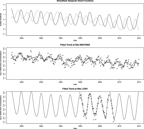
Figure 3: (Top) Two temporal basis functions estimated by modified singular value decomposition from Los Angeles monitoring data; (middle and bottom) raw log-transformed data and fits to the two temporal basis functions at sites near (LC001) and far (06037002) from the coastline.

Last, we specify the model for the residual field, $\nu(s,t)$. Consistent with Lindström et al. (2013), Szpiro et al. (2010), Sampson et al. (2011), we assume that the mean model accounts for the mean structure and all temporal correlation. Thus, the spatio-temporal residuals are assumed to have zero mean and to be independent in time, so that

$$\nu(\mathbf{s},t)\sim N\bigl{(}\mathbf{0},\Sigma_{\nu}^{t}(\bolds{\theta}_{\nu})\bigr{)},$$

where $\Sigma_{\nu}^{t}(\bolds{\theta}_{\nu})$ is a covariance matrix of dimension $n_{t}\times n_{t}$ and $n_{t}$ is the number of sites observed at time $t$ with $\sum_{t}n_{t}=N$, the total number of observations. Once again, we assume that the $\nu$ field follows a spatial exponential decay model with range $\phi$, partial sill $\tau^{2}$ and (possibly) nugget $\sigma^{2}$.

A concise representation of this model is given as

$$\mathbf{Y}=\mathbf{F}\mathbf{X}\bolds{\alpha}+\mathbf{F}\mathbf{B}+\mathbf{F}\mathbf{P}+\mathbf{V},$$ (1)

where $\mathbf{Y}$ is an $N\times 1$ vector of stacked responses $y(s,t)$ (first varying $s$ then $t$), $\mathbf{F}=(f_{st,is^{\prime}})$ is an $N\times mn$ matrix that has elements

$$f_{st,is^{\prime}}=\cases{f_{i}(t),&\quad$\mbox{if }s=s^{\prime}$,\cr 0,&\quad\mbox{else},}$$

$\mathbf{X}$ is a block diagonal matrix with diagonal blocks $\{\mathbf{X}_{j}\}_{j=1}^{m}$, $\bolds{\alpha}$ is an$\sum_{j=1}^{m}\{p_{j}+1\}\times 1$ stacked vector of the $\bolds{\alpha}_{j}$, $\mathbf{B}$ is an $mn\times 1$ vector of the stacked ${\beta}_{j}$, $\mathbf{P}$ is an $mn\times 1$ vector of the stacked nuggets, $\psi_{j}$, and $\mathbf{V}$ is an $N\times 1$ vector of the stacked ${\nu}$ (first varying $s$ then $t$). This model is thus indexed by the land use regression coefficients, $\bolds{\alpha}$, and the covariance parameters

$$\bolds{\theta}_{B} = (\bolds{\theta}_{1},\ldots,\bolds{\theta}_{m}),\qquad\bolds{\theta}_{j}=\bigl{(}\phi_{j},\tau^{2}_{j}\bigr{)},\qquad j=1,\ldots,m,$$

$$\bolds{\theta}_{P} = \bigl{(}\sigma^{2}_{1},\ldots,\sigma^{2}_{m}\bigr{)},$$

$$\bolds{\theta}_{V} = \bigl{(}\phi_{\nu},\tau^{2}_{\nu},\sigma^{2}\bigr{)}.$$

To simplify notation, we collect the covariance parameters into the vector $\bolds{\Xi}=(\bolds{\theta}_{B},\bolds{\theta}_{P},\bolds{\theta}_{V})$. In the remainder of the manuscript, for the sake of brevity we suppress the dependence of covariance matrices on their respective parameters, except where an explicit dependence is illustrative.

Model (1) is typically fit using profile maximum likelihood methods, although full maximum likelihood and restricted maximum likelihood approaches are also possible [Lindström et al. (2013)]. Sampson used a multi-stage “pragmatic” approach to fitting (1) and generating predictions [Sampson et al. (2011)]. Lindström adapted the model to allow for time-varying covariates, although this extension is not presented here [Lindström et al. (2013)]. This model is implemented in the R-package, SpatioTemporal, available at http://cran.r-project.org/package=SpatioTemporal.

3.2 Motivation for reduced-rank spatial smoothing

Although the above formulation of the model has been successful for predicting air pollution concentrations, we note two limitations of this formulation, particularly with respect to the $\beta$-fields. First, we note that it is not natural to interpret the $\beta$-fields as random effects since it is difficult to imagine the data generating mechanism that might give rise to such fields [Hodges and Clayton (2011), Hodges (2013)]. Second, the range parameters in the $\beta$-fields tend to be challenging to estimate in practice. Moreover, Zhang showed that in the case of spatial generalized linear mixed models, this quantity is not consistently estimable [Zhang (2004)].

As such, we consider a spline-based representation of the $\beta$-fields in the mean model. To motivate, we note that the Gaussian spatial $\beta$-fields, as defined above, can be represented as spatial splines as follows. Let

$$\Sigma_{\beta_{j}}=\tau^{2}_{j}\bolds{\Omega},$$

where $\bolds{\Omega}$ is a matrix such that

$$\bolds{\Omega}=\bigl{\{}C\bigl{(}\|\mathbf{s}_{i}-\mathbf{s}_{j}\|\bigr{)}\bigr{\}}_{i,j\in\mathcal{S}}$$

and $\mathcal{S}$ is the set of observed spatial locations. For the exponential model, $C(r)=\exp\{-|r|/\phi\}$. It follows that the $\beta$-fields can be expressed as

$$\beta_{j}(\mathbf{s})=\bolds{\Omega}^{1/2}\bolds{\delta}_{j},$$

where $\bolds{\delta}_{j}\sim\operatorname{MVN}(\mathbf{0},\tau^{2}_{j}\mathbf{I})$. The $n$ columns of the matrix $\bolds{\Omega}^{1/2}$ represent $n$ spatial basis functions indexed by the parameter $\phi_{j}$. Written as such, the $\beta$-fields can be viewed as random linear combinations of spatial basis functions. Exploiting the connection between linear mixed models and penalized splines, we can view the $\beta_{j}$-fields as penalized spatial splines with smoothing parameters $\sigma^{2}/\tau^{2}_{j}$ [Ruppert, Wand and Carroll (2003)]. Having represented the $\beta$-fields as penalized splines, it is natural to consider penalized reduced-rank splines instead as a means of improving model performance and computational efficiency.

We note that an analogous argument can be made for the residual field. However, it is also the case that the $\nu$-field is well understood within the traditional framework of random effects models. That is, the $\nu$-field captures extra random spatial variation that arises from time point to time point. Furthermore, the range parameter in the $\nu$-field tends to be more stably estimated in practice due to the repeated measurements over time.

In the following sections, we describe reduced-rank representations of the $\beta$-fields using low-rank kriging and thin plate regression splines.

3.3 Low-rank kriging

We follow the approach outlined by Kammann and Wand (2003) and Ruppert, Wand and Carroll (2003) for low-rank kriging (LRK) of the $\beta$-fields. Specifically, LRK is achieved by replacing $\bolds{\Omega}$ with $\mathbf{Z}\tilde{\bolds{\Omega}}{}^{-1}\mathbf{Z}^{\top}$, where

$$\mathbf{Z}=\bigl{\{}C\bigl{(}\|\mathbf{s}_{i}-\bolds{\kappa}_{j}\|\bigr{)}\bigr{\}}_{i\in\mathcal{S},j\in\mathcal{K}},\qquad\tilde{\bolds{\Omega}}=\bigl{\{}C\bigl{(}\|\bolds{\kappa}_{i}-\bolds{\kappa}_{j}\|\bigr{)}\bigr{\}}_{i,j\in\mathcal{K}},$$

and $\mathcal{K}$ is the set of spatial knot locations, $\bolds{\kappa}$, of cardinality $K\ll n$. It follows that we can approximate $\beta_{j}(\mathbf{s})$ by $\mathbf{Z}\tilde{\bolds{\Omega}}{}^{-1/2}\bolds{\delta}_{j}$, where $\bolds{\delta}_{j}$ is now a $K$-vector distributed as $\operatorname{MVN}(0,\Sigma_{\delta_{j}}=\tau^{2}_{j}\mathbf{I})$. We note that this approach bears strong resemblance to the predictive processes presented by Banerjee [Banerjee et al. (2008)]. In fact, Banerjee noted that LRK is a re-projection of his predictive process. As such, these approaches are computationally identical despite the fact that the predictive process is derived formally from a full-rank parent process.

Letting $\mathbf{Z}_{B}=\{\mathbf{Z}\tilde{\bolds{\Omega}}{}^{-1/2}\}_{j=1}^{m}$ and $\tilde{\mathbf{B}}$ be the stacked vector of $\bolds{\delta}_{j}$s, we can express the spatio-temporal model as

$$Y=\mathbf{F}\mathbf{X}\bolds{\alpha}+\mathbf{F}\mathbf{Z}_{B}\tilde{\mathbf{B}}+\mathbf{F}\mathbf{P}+\mathbf{V}.$$ (2)

Model (2) can be re-expressed as

$$\mathbf{Y}\sim\operatorname{MVN}(\mathbf{F}\mathbf{X}\bolds{\alpha},\tilde{\Sigma}),$$

where

$$\tilde{\Sigma}=\mathbf{F}\mathbf{Z}_{B}\Sigma_{\tilde{B}}\mathbf{Z}_{B}^{\top}\mathbf{F}^{\top}+\mathbf{F}\Sigma_{P}\mathbf{F}^{\top}+\Sigma_{V},$$

$\Sigma_{\tilde{B}}$ is a block-diagonal matrix with diagonal elements $\{\Sigma_{\delta_{j}}\}_{j=1}^{m}$, $\Sigma_{P}$ is a block-diagonal matrix with diagonal elements $\{\sigma^{2}_{j}\mathbf{I}_{n}\}_{j=1}^{m}$, and $\Sigma_{V}$ is a block-diagonal matrix with diagonal elements $\{\Sigma_{\nu}^{t}\}_{t=1}^{T}$. The log-likelihood is given by

$$l(\bolds{\alpha},\bolds{\Xi}\mid\mathbf{Y})\propto-\log|\tilde{\Sigma}|-(\mathbf{Y}-\mathbf{F}\mathbf{X}\bolds{\alpha})^{\top}\tilde{\Sigma}^{-1}(\mathbf{Y}-\mathbf{F}\mathbf{X}\bolds{\alpha}).$$

Consistent with Szpiro et al. (2010), Lindström et al. (2013), we estimate regression coefficients $\bolds{\alpha}$ using the profile maximum likelihood. It is easy to show that

$$\hat{\bolds{\alpha}}=\bigl{(}\mathbf{X}^{\top}\mathbf{F}^{\top}\tilde{\Sigma}^{-1}\mathbf{F}\mathbf{X}\bigr{)}^{-1}\mathbf{X}^{\top}\mathbf{F}^{\top}\tilde{\Sigma}^{-1}\mathbf{Y},$$

so that the profile log likelihood is simplified to

$$l_{p}(\bolds{\Xi}\mid\mathbf{Y})\propto-\log|\tilde{\Sigma}|-(\mathbf{Y}-\mathbf{F}\mathbf{X}\hat{\bolds{\alpha}})^{\top}\tilde{\Sigma}^{-1}(\mathbf{Y}-\mathbf{F}\mathbf{X}\hat{\bolds{\alpha}}),$$ (3)

and the remaining parameters are estimated as those quantities that maximize (3). We estimate all parameters using the L-BFGS-B algorithm as implemented in the optim function in stats package in R. This is an iterative method that allows for box constraints on all parameters [Byrd et al. (1995)].

Prediction is achieved by assuming a joint distribution between observed data $\mathbf{Y}$ and unobserved data $\mathbf{Y}^{*}$,

$$\pmatrix{\mathbf{Y}\cr\mathbf{Y}^{*}}\sim\left(\pmatrix{\mathbf{F}\mathbf{X}\cr\mathbf{F}^{*}\mathbf{X}^{*}}\bolds{\alpha},\left[\matrix{\tilde{\Sigma}&\tilde{\Sigma}_{\cdot*}\cr\tilde{\Sigma}_{*\cdot}&\tilde{\Sigma}_{**}}\right]\right),$$

where $\tilde{\Sigma}_{**}$ is the covariance of $\mathbf{Y}^{*}$ and $\tilde{\Sigma}_{\cdot*}$ is the cross covariance of $\mathbf{Y}$ and $\mathbf{Y}^{*}$. Predictions are based on the conditional expectation $E[\mathbf{Y}^{*}|\mathbf{Y}]$ with MLEs plugged in, namely,

$$\hat{\mathbf{Y}}^{*}=\mathbf{F}^{*}\mathbf{X}^{*}\hat{\bolds{\alpha}}+\hat{\tilde{\Sigma}}_{*\cdot}\hat{\tilde{\Sigma}}{}^{-1}(\mathbf{Y}-\mathbf{F}\mathbf{X}\hat{\bolds{\alpha}})$$

with conditional prediction variance

$$V\bigl{(}\mathbf{Y}^{*}\mid\mathbf{Y},\hat{\Xi},\hat{\bolds{\alpha}}\bigr{)}=\hat{\tilde{\Sigma}}_{**}-\hat{\tilde{\Sigma}}{}^{\top}_{*\cdot}\hat{\tilde{\Sigma}}{}^{-1}\hat{\tilde{\Sigma}}_{\cdot*}.$$

A drawback of LRK is the dependence of the basis functions on the range parameters $\phi_{j},j=1,\ldots,m$. Kammann and Wand, for purely spatial data, address this issue by fixing the value of this parameter at the maximum spatial distance observed in the data [Kammann and Wand (2003)]. Although it is attractive to condition on fixed spatial basis functions, arbitrary selection of these parameters could lead to worse predictive performance. The range parameters can be estimated from the data, albeit at the expense of more challenging numerical optimization and with the caveat that they may not be consistently estimable [Zhang (2004)].

An alternative approach which sidesteps these issues and leverages the spatial spline formulation calls for the use of alternative spline bases. Thin plate regression splines are a popular alternative, and we explore their application in the current problem below.

3.4 Summary of thin plate regression splines

Thin plate regressionsplines (TPRS) present an alternative to the LRK approach and mitigate the issue of estimating the range parameter(s) [Wood (2003)]. Although these models are widely used (implementation is available in the R package mgcv, e.g.), we briefly summarize the approach with the goal of describing parallels between TPRS and LRK.

Assume that we wish to estimate the function $f$ based on (purely spatial) observations $\mathbf{Y}$ at locations $\mathbf{s}=(s_{1},s_{2})$ such that

$$Y_{i}=f(s_{i})+\varepsilon_{i}$$

by minimizing this penalized objective function

$$\bigl{\|}\mathbf{Y}-f(\mathbf{s})\bigr{\|}+\lambda\int_{s_{1}}\!\int_{s_{2}}\biggl{(}\frac{\partial^{2}f}{\partial s_{1}^{2}}+\frac{\partial^{2}f}{\partial s_{2}^{2}}+\frac{\partial^{2}f}{\partial s_{1}\,\partial s_{2}}\biggr{)}^{2}\,ds_{1}\,ds_{2}.$$

It can be shown that the solution is given by

$$f(s)=\sum_{i=1}^{n}\zeta_{i}\eta\bigl{(}\|s-s_{i}\|\bigr{)}+\sum_{j=1}^{3}\gamma_{j}\iota_{j}(s),$$ (4)

where the $\iota_{j}$ are linearly independent polynomials spanning the space of polynomials in $\mathcal{R}^{2}$ (of degree less than $2$) and $\eta(r)=2^{-3}\pi^{-1}r^{2}\log(r)$. Further, $\bolds{\zeta}$ and $\bolds{\gamma}$ are fixed unknown coefficients subject to the constraint $\mathbf{T}^{\top}\bolds{\zeta}=0$ with $T_{ij}=\iota_{j}(s_{i})$ [Green and Silverman (1994)].

Let $\mathbf{E}$ be a matrix so that $E_{ij}=\eta(\|s_{i}-s_{j}\|)$. Wood presents a reduced-rank approximation of this problem, which is the solution to the unconstrained optimization problem

$$\operatorname{minimize}\bigl{\|}\mathbf{Y}-\mathbf{U}_{K}\mathbf{D}_{K}\mathbf{W}_{K}\bolds{\zeta}^{*}-\mathbf{T}\bolds{\gamma}\bigr{\|}+\lambda\bolds{\zeta}^{*\top}\mathbf{W}_{K}^{\top}\mathbf{D}_{K}\mathbf{W}_{K}\bolds{\zeta}^{*},$$

where $\bolds{\zeta}^{*}$ is a $K-3\times 1$ vector of fixed unknown coefficients, $\mathbf{U}\mathbf{D}\mathbf{U}^{\top}$ is the eigendecomposition of $\mathbf{E}$ so that the $n$ columns of $\mathbf{U}$ are equal to the eigenvectors of $\mathbf{E}$ ordered by their associated eigenvalues from largest to smallest, $\mathbf{D}$ is a diagonal matrix of these eigenvalues, $\mathbf{U}_{K}$ is a matrix of the first $K$ columns of $\mathbf{U}$, and $\mathbf{D}_{K}$ is a matrix of the first $K$ rows and columns of $\mathbf{D}$. Last, $\mathbf{W}_{K}$ is a $K\times K-3$ orthogonal column basis such that $\mathbf{T}^{\top}\mathbf{U}_{K}\mathbf{W}_{K}=\mathbf{0}$ (to account for the constraint) [Wood (2003)].

It is easy to see that this unconstrained optimization is equivalent to fitting the linear mixed model

$$\mathbf{Y}=\mathbf{T}\bolds{\gamma}+\mathbf{U}_{K}\mathbf{D}_{K}\mathbf{W}_{K}\bolds{\zeta}^{*}+\bolds{\varepsilon},$$

where $\bolds{\zeta}^{*}\sim\operatorname{MVN}(\mathbf{0},\sigma^{2}_{\zeta}(\mathbf{W}_{K}^{\top}\mathbf{D}_{K}\mathbf{W}_{K})^{-1})$, $\bolds{\varepsilon}\sim\operatorname{MVN}(\mathbf{0},\sigma^{2}_{\varepsilon}\mathbf{I})$, and $\lambda=\sigma^{2}_{\varepsilon}/\sigma^{2}_{\zeta}$. Equivalently, let $\bolds{\zeta}^{*}=(\mathbf{W}_{K}^{\top}\mathbf{D}_{K}\mathbf{W}_{K})^{-1/2}\bolds{\delta}^{*}$, where $\bolds{\delta}^{*}\sim\operatorname{MVN}(0,\sigma^{2}_{\zeta}\mathbf{I})$, then the above equation becomes the following:

$$\mathbf{Y}=\mathbf{T}\bolds{\gamma}+\mathbf{U}_{K}\mathbf{D}_{K}\mathbf{W}_{K}\bigl{(}\mathbf{W}_{K}^{\top}\mathbf{D}_{K}\mathbf{W}_{K}\bigr{)}^{-1/2}\bolds{\delta}^{*}+\bolds{\varepsilon}.$$

3.5 Formulation of $\beta$-fields as thin plate regression splines

We consider modeling the $\beta$-fields as TPRS using the relationship between penalized splines and mixed models [Ruppert, Wand and Carroll (2003)]. Following the above formulation, we can approximate $\beta_{j}(\mathbf{s})$ in (1) as $\mathbf{T}\bolds{\gamma}_{j}+\mathbf{Z}^{*}\bolds{\delta}_{j}^{*}$, where $\mathbf{T}$ contains the spatial coordinates of the monitoring locations, $\bolds{\gamma}_{j}$ is a $2\times 1$ vector of fixed unknown coefficients, $\mathbf{Z}^{*}=\mathbf{U}_{K}\mathbf{D}_{K}\mathbf{W}_{K}(\mathbf{W}_{K}^{\top}\mathbf{D}_{K}\mathbf{W}_{K})^{-1/2}$, and $\bolds{\delta}^{*}_{j}$ is a $K-3\times 1$ vector distributed as $\operatorname{MVN}(\mathbf{0},\tau^{2}_{j}\mathbf{I})$.

We can succinctly incorporate this approximation into our modeling framework as follows. First, augment the design matrices $\mathbf{X}_{j}$ by appending the matrix $\mathbf{T}$ so that $\mathbf{X}^{*}_{j}=(\mathbf{X}_{j}\ \mathbf{T})$ for $j=1,\ldots,m$ (if $\mathbf{X}_{j}$ already contains the spatial coordinates as predictors, then this step is unnecessary). Additionally, append the vector $\bolds{\gamma}_{j}$ to the $\bolds{\alpha}_{j}$ so that $\bolds{\alpha}^{*\top}_{j}=(\bolds{\alpha}_{j}^{\top}\ \bolds{\gamma}^{\top}_{j})$ for $j=1,\ldots,m$. Last, letting $\mathbf{Z}^{*}_{B}$ be a block-diagonal matrix with diagonal elements $\{\mathbf{Z}^{*}\}_{j=1}^{m}$ and $\bolds{\alpha}^{*}$ and $\tilde{\mathbf{B}}^{*}$ be the stacked vectors of $\bolds{\alpha}_{j}^{*}$ and $\bolds{\delta}_{j}^{*}$ for $j=1,\ldots,m$, respectively, we formulate the TPRS version of the spatio-temporal model as a linear mixed model, as follows:

$$\mathbf{Y}=\mathbf{F}\mathbf{X}^{*}\bolds{\alpha}^{*}+\mathbf{F}\mathbf{Z}^{*}_{B}\tilde{\mathbf{B}}^{*}+\mathbf{F}\mathbf{P}+\mathbf{V}.$$ (5)

We note the similarities between equations (2) and (5). In fact, Nychka showed that thin plate splines are equivalent to kriging using a generalized covariance function [Nychka (2000)]. It is clear that the difference between LRK and TPRS has to do primarily with the choice of basis functions. However, we also emphasize that the TPRS bases are not dependent on any additional (e.g., range) parameters. Estimation of model parameters and prediction follows as described in Section 3.3.

4 Computational considerations

Evaluation of (3) directly is computationally intensive, with the number of computations growing as $\mathcal{O}(N^{3})$. However, the computational burden can be eased considerably by taking advantage of the block-diagonal nature of the $\Sigma_{B}$ and $\Sigma_{V}$. Namely, Lindström showed that reformulation of (3) can reduce the computational burden to $\mathcal{O}(m^{3}n^{3})$ [Lindström et al. (2013)]. Typically, low-rank models boast a computational advantage over their full-rank counterparts. Yet, reducing the computational burden in spatio-temporal data is nuanced. In the following, we discuss how the formulation of the $\beta$-fields using either LRK or TPRS impacts computation. We illustrate the computational burden of calculating (3) by considering the determinant term $|\tilde{\Sigma}|$, employing a similar reformulation to that employed in Lindström et al. (2013) to exploit the block diagonal nature of $\Sigma_{B}$ and $\Sigma_{V}$. Proofs of the following results and the corresponding reformulation of the full likelihood in (3) are provided in the Online Supplement [Olives et al. (2014)].

By application of known identities, it can be shown that

$$\quad|\tilde{\Sigma}| = \bigl{|}\mathbf{F}\mathbf{Z}_{B}\Sigma_{\tilde{B}}\mathbf{Z}_{B}^{\top}\mathbf{F}^{\top}+\mathbf{F}\Sigma_{P}\mathbf{F}^{\top}+\Sigma_{V}\bigr{|}$$

$$= |\Sigma_{\tilde{B}}||\Sigma_{P}||\Sigma_{V}|\bigl{|}\Sigma_{P}^{-1}+\mathbf{F}^{\top}\Sigma_{V}^{-1}\mathbf{F}\bigr{|}$$

$${}\times\bigl{|}\Sigma_{\tilde{B}}^{-1}+\mathbf{Z}_{B}^{\top}\mathbf{F}^{\top}\bigl{(}\Sigma_{V}^{-1}-\Sigma_{V}^{-1}\mathbf{F}\bigl{(}\mathbf{F}^{\top}\Sigma_{P}^{-1}\mathbf{F}+\Sigma_{V}^{-1}\bigr{)}^{-1}\mathbf{F}^{\top}\Sigma_{V}^{-1}\bigr{)}\mathbf{F}\mathbf{Z}_{B}\bigr{|}.$$

For highly unbalanced data like that which we typically encounter in MESA Air, (4) is dominated by the calculation of $|\Sigma_{P}^{-1}+\mathbf{F}^{\top}\Sigma_{V}^{-1}\mathbf{F}|$. Computation of this component grows at $\mathcal{O}(m^{3}n^{3})$, the same rate as the full-rank model.

As mentioned, the full-rank spatio-temporal model originally published by Szpiro did not include the nugget, $\mathbf{P}$, in the $\beta$-fields [Szpiro et al. (2010)]. When the nugget is not present, the determinant $|\tilde{\Sigma}|$ reduces to

$$|\tilde{\Sigma}| = \bigl{|}\mathbf{F}\mathbf{Z}_{B}\Sigma_{\tilde{B}}\mathbf{Z}_{B}^{\top}\mathbf{F}^{\top}+\Sigma_{V}\bigr{|}$$

$$= |\Sigma_{\tilde{B}}||\Sigma_{V}|\bigl{|}\Sigma_{\tilde{B}}^{-1}+\mathbf{Z}_{B}^{\top}\mathbf{F}^{\top}\Sigma_{V}^{-1}\mathbf{F}\mathbf{Z}_{B}\bigr{|}.$$

Interestingly, in (LABEL:eqdet2), computation will generally be dominated by calculation of $|\tilde{\Sigma}_{B}^{-1}+\mathbf{Z}_{B}^{\top}\mathbf{F}^{\top}\Sigma_{V}^{-1}\mathbf{F}\mathbf{Z}_{B}|$, which grows at $\mathcal{O}(m^{3}K^{3})$. This makes it clear that, when the nugget is not present, reducing the rank of the $\beta$-fields can lead to some improvement in terms of computation. We note that in the case where the data are more balanced, it is possible that computation of $|\Sigma_{V}|$ (or, equivalently, $\Sigma_{V}^{-1}$), which grows at $\mathcal{O}(\sum_{t}n_{t}^{3})$, will dominate computation in both cases.

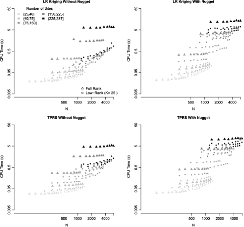
Figure 4: CPU time required for a single log-likelihood evaluation of LRK and TPRS models for the EPA AQS and MESA Air NO_x monitoring data in Los Angeles, California. Triangles indicate models where the rank of the spatial smooth is equal to the number of sites and circles indicate models where the rank of the smooth is equal to 25 in various depleted MESA Air data sets.

In Figure 4, we plot the CPU time required for optimized log-likelihood evaluation in full-rank and reduced-rank models with $K=25$ with and without the nugget present for both LRK and TPRS. We see that for LRK and TPRS, as the number of sites increases, full-rank models take large steps in computation time required, whereas reduced-rank models grow much more slowly when a nugget is not present. However, there is very little difference in computational growth between full- and reduced-rank models as the number of sites increases when the nugget is present.

5 Application to NO_x monitoring data in Los Angeles

We apply the proposed reduced-rank spatio-temporal models to NO_x data collected in the Los Angeles area as part of the MESA Air monitoring campaign and via the EPA regulatory network.

5.1 Models considered

We fit a variety of models to the data which vary in three aspects: (1) the choice of spline basis, (2) the rank of $\beta$-field smooth, and (3) the inclusion of the nugget. In all models considered, we employ two time trends ($m=2$) as depicted in Figure 3. Likewise, the residual $\nu$-field is always specified as exponentially distributed with a nugget. And, last, all of the GIS covariates are present in each of the $\mathbf{X}_{j}$ matrices.

5.1.1 Choice of spline basis

We have outlined two possible classes of spline bases, exponential (used in LRK) and thin plate splines. As previously indicated, the use of exponential basis functions requires handling of the range parameters in each of the $\beta$-fields by either fixing its value at some ad hoc data-derived value or through full optimization. To investigate the trade-off between optimization of an additional range parameter and fixing this parameter at an arbitrary conservative value, we assume the range parameters in the $\beta$-fields are both fixed, and in separate models that they are estimated. To assess the sensitivity to the fixed value, we set the range parameters in all fields equal to the maximum, one half, one quarter and one eighth of the observed maximum spatial range in the data (80.7 km). Additionally, to assess the sensitivity of model performance to the choice of spline basis, we fit TPRS smooths to the $\beta$-fields.

5.1.2 Rank of smooth

As a general rule of thumb, Ruppert, Wand and Carroll suggest that the number of knots, $K$, be chosen as $\max(20,\min\{150,\break n/4\})$ [Ruppert, Wand and Carroll (2003)]. In the case of our MESA Air and EPA data, this would result in $K=71$. Although this rule of thumb is convenient, it is unclear how the number of knots in the spatial component of the mean model will influence spatio-temporal prediction. For our purposes, we explore a variety of different ranks on spatio-temporal prediction, $K=287,100,50$ and $25$. We note that the models with $K=287$ correspond to full-rank models.

Knot location can also play an important role in LRK. Kammann and Wand choose knot locations using efficient space-filling algorithms [as implemented by the cover.design() function in the R package fields] [Kammann and Wand (2003)]. In our primary investigations, we choose knot locations using space-filling of monitoring sites within the study area (see Figure 5). Although space-filling of observed locations is a convenient approach to choosing the knot locations in our analysis, it is natural to consider knots chosen at alternative locations. For example, an attractive option could be to specify knot locations on a regular grid over the study area. To investigate, in addition to the primary analysis, we also fit models where knot locations are chosen using space-filling of a regular grid of the convex hull of the study region, where each grid cell is approximately 2.5 kilometers on each side (see Figure 5).

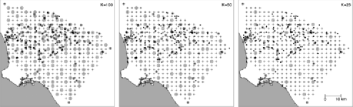
Figure 5: Map of knot locations chosen by efficient space-filling of monitoring locations (small open circle) and of regular grid locations (large open circles). Small black dots represent participant locations and crosses represent grid locations. “Home outdoor” monitors have been jittered for participant confidentiality.

5.1.3 Nugget effect

Given the analytical findings suggesting thatreduced-rank modeling leads to a computational advantage in the case when the nugget is not present, we fit models both with and without the nugget. However, we note that while analytically feasible, models which exclude the nugget from the $\beta$-fields are less conceptually defensible. Namely, exclusion of the nugget from the $\beta$-fields makes it difficult for the model to capture fine-scale variability in the mean process. Moreover, preliminary investigations showed that very low-rank smooths in models without a nugget in the $\beta$-fields were unstable. As such, we present a limited set of results for reduced-rank models where the nugget is not present.

5.2 Model validation

We employ cross-validation to assess model predictive performance. Our primary interest is in prediction of long-term averages of NO_x concentrations. Unfortunately, in this data set there are only 26 AQS and/or MESA “fixed sites” that provide adequately long time-series for long-term average validation. These sites tend to be more homogeneous in their geographic covariate distribution and have larger spatial spread when compared to MESA participant locations, which could potentially limit our ability to adequately assess predictive performance.

As such, in addition to cross-validation of AQS and MESA “fixed sites,” we also consider cross-validation of MESA “community snapshot” and “home outdoor” sites. We apply tenfold cross-validation to each type of monitor. In each of these three scenarios, all remaining data are used to estimate model parameters and to predict at left-out locations.

Due to the varying nature of sampling at sites in each of the three scenarios, Lindström suggests calculating RMSE and $R^{2}$ slightly differently in each case [Lindström et al. (2013)]. At “fixed”/AQS sites, we calculate RMSE and $R^{2}$ metrics on both the 2-week and long-term average scales. Long-term averages at left-out sites are computed only over times where data are observed, so that

$$c(s)=\sum_{\tau\dvtx\exists y(s,\tau)}\frac{\exp\{y(s,\tau)\}}{|\{t\dvtx\exists y(s,t)\}|}.$$

The cross-validated $R^{2}$ on the long-term average scale is given by [Szpiro, Sheppard and Lumley (2011)]

$$R^{2}=\min\biggl{\{}0,1-\frac{\operatorname{RMSE}(\hat{c}(s))^{2}}{\operatorname{Var}(c(s))}\biggr{\}}.$$ (8)

For the second scenario, we perform cross-validation of the “community snapshot” locations. We cross-validate all three sampling periods/seasons simultaneously and calculate cross-validated RMSE and $R^{2}$ by season. Doing so allows us to assess the spatial predictive ability of the model across multiple seasons. Likewise, as each of the “community snapshot” locations were sampled during the same two-week periods, we can view the resulting metrics as representative of the pure spatial predictive capacity of the model.

Last, we also consider cross-validation of “home outdoor” sites. As the “home outdoor” sites are repeatedly sampled over time and typically at different time points, much of the $R^{2}$ is likely to reflect a temporal signal, which is strong in these data. As such, in addition to the raw cross-validated $R^{2}$, we also consider a de-trended version of the $R^{2}$ where the variance, $\operatorname{Var}(c(s))$, in (8) is replaced by the variance of observations after removing the predictions from a reference model that accounts for (some) temporal variability. Here, we use a reference model based on the spatial average of measurements at AQS/“fixed sites” at each time point. Thus, the de-trended $R^{2}$ represents the improvement in performance of our models compared to central site predictions commonly used in air pollution epidemiology studies [Pope et al. (1995)].

5.3 Comparison with other reduced-rank spatio-temporal models

Al-though the current model was developed specifically to address the complexities arising in the context of MESA Air, a number of other methods for reduced-rank spatial and spatio-temporal modeling have been published, including fixed-rank filtering, Gaussian Markov random field approximations, covariance tapering, predictive processes and generalized additive models. Unfortunately, fixed-rank filtering is not available in an off-the-shelf package, and implementing this model for these data is a project unto itself. We further note that the application of Gaussian Markov random field approximations and covariance tapering in this setting is nuanced and may not result in any computational savings for these data. See the Online Supplement [Olives et al. (2014)] for further discussion of the application of these two approaches in the current modeling framework.

As mentioned previously, there appears to be an explicit correspondence between predictive processes and LRK, as noted in Banerjee et al. (2008). As such, formally modeling the $\beta$-fields in (1) as reduced-rank predictive processes would not provide any additional insight into this work. That being said, one version of a predictive process spatio-temporal model is implemented in the spBayes package in R. Namely, the function spDynLM fits the following model:

$$y(s,t) = \mathbf{X}_{t}(\mathbf{s})\beta_{t}+u_{t}(\mathbf{s})+\varepsilon_{t}(\mathbf{s}),\qquad t=1,2,\ldots,T,$$

$$\varepsilon_{t}(\mathbf{s}) \sim N\bigl{(}0,\tau_{t}^{2}\bigr{)},$$

$$\beta_{t} = \beta_{t-1}+\eta_{t},\qquad\eta_{t}\sim N(0,\Sigma_{\eta}),$$

$$\beta_{0} \sim N(m_{0},\Sigma_{0}),$$

$$u_{t}(\mathbf{s}) = u_{t-1}(\mathbf{s})+w_{t}(\mathbf{s}),\qquad w_{t}(\mathbf{s})\sim\operatorname{GP}\bigl{(}0,C_{t}(\cdot,\theta_{t})\bigr{)},$$

$$u_{0}(s) = 0.$$

The spatial process $w_{t}$, here assumed to be exponential, can be replaced with a predictive process of reduced rank to reduce computational burden. This model significantly deviates from our own and may not perform well in the context of such highly imbalanced data as that which we analyze here. Nevertheless, we apply it to our data in an effort to make a fair comparison between published approaches to reduced-rank spatio-temporal modeling and our method. Specifically, we fit two models: [2.]

full-rank model ($K=287$) for all $w_{t}$ fields, and

reduced-rank ($K=50$) for all $w_{t}$ with knots chosen on a grid. We note that the spDynLM function requires that knots be chosen on a grid when utilizing the reduced-rank predictive process machinery. In both cases, we fit the models assuming the following priors for the $\theta_{t},\Sigma_{\eta},\tau^{2}_{t}$:

$$1/\phi_{t} \sim \operatorname{Unif}\bigl{(}1/(0.9\times\mbox{max distance}),3/(0.05\times\mbox{max distance})\bigr{)},$$

$$\sigma^{2}_{t} \sim \operatorname{InvGamma}(2,10),$$

$$\tau^{2}_{t} \sim \operatorname{InvGamma}(2,5),$$

$$\Sigma^{2}_{\eta} \sim \operatorname{InvWish}(2,0.001\mathbf{I}_{p}).$$

These priors are largely based on the example code available in the spDynLM documentation, with some small changes to reflect the data. Model predictions were the median of 500 posterior draws, after a burn-in period of 1500. We cross-validated these models for “fixed sites” using the same cross-validation groups as before.

Last, for an additional comparison with methods available in off-the-shelf software, we considered a generalized additive model that reformulates the mean process $\mu(s,t)$ without resorting to a dynamic model. Namely, we replaced $\mu(s,t)$ with the following:

$$\mathbf{X}(\mathbf{s})\bolds{\alpha}+\eta_{t}+g(\mathbf{s})+h(\mathbf{s},t).$$

Here both $g$ and $h$ are modeled using TPRS. For investigating models with spatial rank of $K$, we set the degrees of freedom for $g$ equal to $K$ and the degrees of freedom for $h$ equal to $K\times 14$ (e.g., when $K=50$, $h$ has 700 df), where 14 is the number of years represented in the data. Note that both $g$ and $h$ can be viewed as penalized regression splines with structure similar to what we outline in the paper. But for $h$, we are now assuming a nonseparable model for space and time which differs from the tensor product approach used in our model. Moreover, we do not rely on predefined temporal basis functions to model time. The $\eta_{t}$ are i.i.d. Gaussian random effects that capture nonsmooth temporal variation. Note that the $\nu$-field remains the same as outlined in the paper. We fit this model using the gamm function in the mgcv package in R.

= RMSE $\bolds{R}^{\mathbf{2}}$ Basis$\bolds{/K}$ 287 100 50 25 0 287 100 50 25 0 2-wk LRK ($\phi=\operatorname{est}$) 15.43 15.52 15.72 16.35 17.82 85 85 85 83 80 LRK ($\phi=\max$) 15.64 15.64 15.83 15.87 17.82 85 85 84 84 80 LRK ($\phi=\mathrm{max}/2$) 15.52 15.56 15.24 16.14 17.82 85 85 86 84 80 LRK ($\phi=\mathrm{max}/4$) 15.31 15.32 15.33 15.74 17.82 85 85 85 85 80 LRK ($\phi=\mathrm{max}/8$) 15.04 15.08 15.13 15.59 17.82 86 86 86 85 80 TPRS 16.38 15.29 15.11 16.01 17.82 83 85 86 84 80 LTA LRK ($\phi=\operatorname{est}$) 10.43 10.56 11.11 11.41 12.41 68 67 64 62 55 LRK ($\phi=\max$) 10.48 10.46 10.53 10.84 12.41 68 68 67 65 55 LRK ($\phi=\mathrm{max}/2$) 10.40 10.39 10.08 10.72 12.41 68 68 70 66 55 LRK ($\phi=\mathrm{max}/4$) 10.30 10.31 10.33 11.04 12.41 69 69 69 64 55 LRK ($\phi=\mathrm{max}/8$) 10.26 10.28 10.36 10.85 12.41 69 69 68 65 55 TPRS 10.83 09.99 09.88 10.60 12.41 65 71 71 67 55

Table 2: Cross-validated RMSE and $R^{2}$ for “fixed sites” when nugget is present. $R^{2}$ have been multiplied by 100 for presentation

6 Results

6.1 Performance of proposed reduced-rank models in LA

Table 2 shows the results of the cross-validation at “fixed sites” for models when the nugget is present. For LRK models, the choice of range does not appear to be a strong determinant of the predictive performance, with fully optimized models performing nearly as well as those models with the range parameter fixed at various values. Likewise, TPRS models exhibit highly competitive predictive performance with a slight edge over LRK models at lower ranks for long-term averages. Cross-validated $R^{2}$ values stay relatively consistent across ranks until $K=25$, at which point both 2-week and long-term average predictive scores drop off. In all cases, models with some spatial smoothing ($K>0$) perform better than models without any smoothing ($K=0$).

= RMSE $\bolds{R}^{\mathbf{2}}$ Basis$\bolds{/K}$ 287 100 50 25 0 287 100 50 25 0 Summer LRK ($\phi=\operatorname{est}$) 06.74 06.71 06.73 06.98 06.97 66 66 66 63 63 LRK ($\phi=\max$) 06.68 06.67 07.03 06.70 06.97 66 66 63 66 63 LRK ($\phi=\mathrm{max}/2$) 06.69 06.68 06.66 06.96 06.97 66 66 66 63 63 LRK ($\phi=\mathrm{max}/4$) 06.71 06.72 06.66 06.76 06.97 66 66 66 65 63 LRK ($\phi=\mathrm{max}/8$) 06.76 06.74 06.83 06.82 06.97 65 66 65 65 63 TPRS 06.62 06.71 06.70 06.72 06.97 67 66 66 66 63 Fall LRK ($\phi=\operatorname{est}$) 11.64 11.61 11.99 11.55 11.78 75 76 74 76 75 LRK ($\phi=\max$) 11.66 11.59 11.75 11.83 11.78 75 76 75 75 75 LRK ($\phi=\mathrm{max}/2$) 11.66 11.64 11.61 11.97 11.78 75 75 76 74 75 LRK ($\phi=\mathrm{max}/4$) 11.65 11.63 11.53 11.35 11.78 75 75 76 77 75 LRK ($\phi=\mathrm{max}/8$) 11.66 11.89 11.95 11.86 11.78 75 74 74 74 75 TPRS 11.92 12.10 12.14 12.11 11.78 74 73 73 73 75 Winter LRK ($\phi=\operatorname{est}$) 13.01 12.92 12.98 12.99 15.32 77 77 77 77 68 LRK ($\phi=\max$) 13.04 12.94 13.11 14.00 15.32 77 77 76 73 68 LRK ($\phi=\mathrm{max}/2$) 13.03 12.99 12.59 13.63 15.32 77 77 78 75 68 LRK ($\phi=\mathrm{max}/4$) 13.02 12.98 12.63 13.80 15.32 77 77 78 74 68 LRK ($\phi=\mathrm{max}/8$) 13.05 13.51 12.65 13.95 15.32 77 75 78 73 68 TPRS 13.27 13.04 13.08 14.19 15.32 76 77 77 72 68

Table 3: Cross-validated RMSE and $R^{2}$ for “community snapshot” locations when nugget is present. $R^{2}$ have been multiplied by 100 for presentation

Table 3 show the results of cross-validation at “community snapshot” sites. We typically see the best performance in the Winter as compared with the Fall and Spring seasons. Once again, there appears to be little difference in model performance as the choice of range parameters varies. TPRS models continue to compete strongly with LRK models. The rank of the $\beta$-field smooth does not tend to influence performance heavily, although again spatial smoothing at any rank does tend to improve predictive performance.

= RMSE $\bolds{R}^{\mathbf{2}}$ Basis$\bolds{/K}$ 287 100 50 25 0 287 100 50 25 0 Raw LRK ($\phi=\operatorname{est}$) 5.51 5.52 5.88 5.89 7.03 93 93 92 92 88 LRK ($\phi=\max$) 5.54 5.54 5.71 6.41 7.03 93 93 92 90 88 LRK ($\phi=\mathrm{max}/2$) 5.53 5.54 5.28 6.01 7.03 93 93 93 92 88 LRK ($\phi=\mathrm{max}/4$) 5.53 5.58 5.52 6.14 7.03 93 93 93 91 88 LRK ($\phi=\mathrm{max}/8$) 5.52 5.49 5.48 6.26 7.03 93 93 93 91 88 TPRS 5.52 5.50 5.53 6.00 7.03 93 93 93 92 88 Detrended LRK ($\phi=\operatorname{est}$) 84 84 82 82 75 LRK ($\phi=\max$) 84 84 83 79 75 LRK ($\phi=\mathrm{max}/2$) 84 84 86 81 75 LRK ($\phi=\mathrm{max}/4$) 84 84 84 81 75 LRK ($\phi=\mathrm{max}/8$) 84 84 85 80 75 TPRS 84 84 84 81 75

Table 4: Cross-validated RMSE and $R^{2}$ for “home outdoor” locations when nugget is present. $R^{2}$ have been multiplied by 100 for presentation

Table 4 shows the results of the cross-validation study at “home outdoor” locations. Here, the choice of range parameter model appears to have even less of important role locations than it did at “fixed sites.” Namely, cross-validated RMSE increases only slightly, resulting in a minimal decrease in $R^{2}$, as the rank decreases in the raw home predictions. Detrended $R^{2}$ did show some decay as the rank decreased, but still remained relatively high. TPRS models performed as well as LRK models across ranks. Again, models with some spatial smoothing outperformed those models with no smoothing.

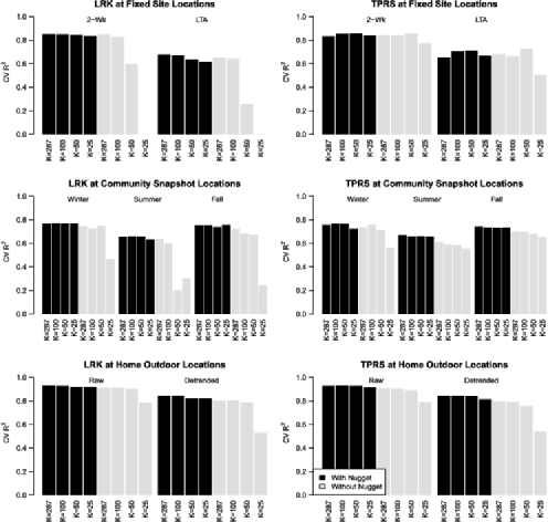
Figure 6: Comparison of cross-validated $R^{2}$ at “fixed site,” “community snapshot,” and “home outdoor” locations using low-rank kriging and TPRS.

Figure 6 compares the cross-validated $R^{2}$ for a set of models of rank $K=287,100,50$ and $25$ with and without the nugget present in the $\beta$-fields at AQS/“fixed sites,” “community snapshot” and “home outdoor” locations. Note, for LRK results, the range parameter has been estimated from the data. The figure suggests that while full rank models ($K=287$) are comparable across these two specifications, predictive performance of models without the nugget in the $\beta$-fields tend to drop off rapidly as the rank of the smooth decreases, particularly in the case of LRK, where in select cases the $R^{2}$ decreases to zero when $K=25$. TPRS models tend to be more robust, although the decrease in $R^{2}$ in TPRS models without a nugget tends to be greater than in TPRS models with a nugget.

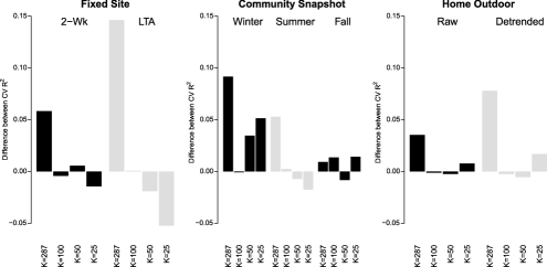
Figure 7: Differences between cross-validated $R^{2}$ in LRK models with knots chosen at monitoring locations and on a regular grid by rank. Models assume that the nugget, $\mathbf{P}$, is present in all $\beta$-fields and the range parameters are estimated by maximum likelihood.

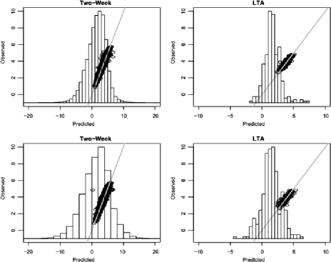
Figure 8: (Top row) In-sample fits for full-rank models fit in spBayes. (Bottom row) In-sample fits for reduced-rank models ($K=50$) fit in spBayes. Histograms represent the distribution of posterior predictions at time points/locations without observed data.

Figure 7 compares the results of fitting full and LRK models to the MESA Air data when the knots were chosen using space-filling of either monitoring locations or a regularly spaced grid of locations. Generally speaking, models where knots were chosen at monitoring sites performed better than those where knots were chosen at grid locations.

6.2 Performance of other reduced-rank spatio-temporal modeling methods

We found that the spDynLM implementation did not work well for our data, possibly due to the large imbalance across space and time. In both models ($K=50,287)$, the time-varying range parameter was not well identified and varied significantly, thus resulting in poor characterization of the rate of spatial decay. The temporal sparsity of the data may also have contributed to the poor performance due to the dynamic nature of the model’s temporal trend. While the in-sample fits for these models are quite good, the out-of-sample predictions are highly variable, resulting in cross-validated $R^{2}$ equal to zero for all scenarios considered. In Figure 8 we show the scatter plots of observed and predicted values in fitted models. The histograms in this same figure represent the distribution of predictions at unobserved times and locations. We note that these are on the log-scale, so that when exponentiated to the native scale, many predicted values at unobserved times/locations are extremely large.

The results of our gamm implementation were only marginally better. While the in-sample fits of this approach were more promising (see Figure 9), the predictions were nowhere near the caliber of those achieved using our model. Inspection of the residuals suggests that there remains significant temporal correlation that is unaccounted for by the mean model. We found that the cross-validated $R^{2}$ was equal to 0 on both the two-week and long-term average scale using this approach. This low $R^{2}$ was driven by the presence of outlying predictions for a handful of sites in two different cross-validation groups. Additionally, the model failed to converge for a single cross-validation group.

Figure 9: In-sample fits for reduced-rank models fit in mgcv with $K=50$ on the two-week scale (left) and long-term average scale (right).

7 Discussion

This paper focuses on presentation of LRK and TPRS representations of the mean process in the spatio-temporal model proposed by Szpiro et al. (2010), Sampson et al. (2011), and Lindström et al. (2013). Our approach allows for a reduced-rank representation of the $\beta$-fields in the mean process of the original model, which tends to be the most time-consuming piece to evaluation in likelihood optimization. In certain cases, we have shown that such reduced-rank representations of the $\beta$-fields can lead to a computational advantage over the full rank specification. Namely, when the nugget of the $\beta$-field is not present, we have shown that our low-rank approach leads to slower growth in the CPU time required for likelihood evaluation.

The formulation of the $\beta$-fields in the mean process of the model as spatial splines is attractive for a number of other reasons. For example, oftentimes predictions of air pollution concentrations are used as inputs into health models to estimate health effects. Typically, the predictions are based on spatially misaligned data and ignoring this fact can lead to biased results and overly optimistic standard errors [Szpiro, Sheppard and Lumley (2011)]. The expression of the $\beta$-fields as splines places GIS covariates and spatial smoothing on more equal footing. Namely, in this form we can think of the GIS covariates and the spatial basis functions as unpenalized and penalized spatial covariates, respectively. This interpretation leads to a more coherent approach to measurement error correction for spatially misaligned data [Szpiro and Paciorek (2013)]. It is also important to note that the computational advantage gained in log-likelihood evaluation extends analogously to prediction, thus reducing computation time needed to predict at potentially many new locations.

For LRK models, we explored the choice of range parameters of prediction, ranging from the case where the range was fully estimated from the data to the case where it was fixed at an arbitrary conservative value indicated by the data. In the scenario when the range parameter is fixed, we showed that the original specification of the full-rank model can also be interpreted as a standard penalized spatial spline.

Likewise, we discussed the parallels between kriging and TPRS. We emphasize that a limitation of the kriging basis functions is the reliance on the range parameter and that TPRS is not subject to the same limitation. That being said, we note that there is an equivalence between thin plate splines and kriging using a Matern-covariance with infinite range [Wahba (1981), Nychka (2000), Kimeldorf and Wahba (1970)]. As such, one might view the use of TPRS as making an implicit assumption about the range parameter. The fact that TPRS and LRK were competitive in our results indicates that TPRS is a valid and attractive option for spatial smoothing in these models. To further this argument, we performed additional analyses (results included in the Online Supplement [Olives et al. (2014)]) comparing out-of-sample prediction variances and AIC as a means of model selection. These analyses indicated that TPRS models tended to result in more stable prediction variances across rank specification when compared to LRK models. However, there was little notable difference between AIC values in LRK and TPRS models. Rather, AIC values indicated full-rank LRK models were preferable to reduced-rank ones in all cases. TPRS models with $K=100$ had the lowest AIC.

Our approach to model assessment relies on cross-validation. As we are primarily interested in prediction of long-term averages, the cross-validation approach outlined isolates the spatial predictive capacity of the models. We applied our approach to ambient MESA Air and EPA NO_x data collected in the Los Angeles area as well as traditional road covariates and Caline point predictions models. We found that generally speaking, the choice of the range parameter in the LRK exponential spatial basis functions had little impact on the model performance. In fact, reducing the rank of the model tended to also have little impact in most cross-validation scenarios for ranks of moderate size ($K=50,100$). We note that the recommendation of Ruppert, Wand and Carroll ($K=71$ for the MESA Air data) falls squarely in this range [Ruppert, Wand and Carroll (2003)]. However, we found that reduction of the rank of the $\beta$-fields below $K=50$ tended to noticeably impact model predictions. This impact was further exacerbated by exclusion of the nugget in the $\beta$-fields. This finding is not a surprise, as exclusion of the nugget in the $\beta$-fields amounts to attributing all extra variation in the mean beyond what is explained by the GIS covariates to the spatial $\beta$-fields. Reduction of the rank of the smooth of these random fields results in a spatial smooth that is unlikely to be able to capture spatial heterogeneity.

This unfortunate finding is at odds with the goal of reducing the computational burden of full-rank spatio-temporal likelihood evaluations. Although the original specification published by Szpiro et al. did not include a nugget in the $\beta$-field, it is our feeling that such models are less defensible than those that include a nugget, since it is unlikely that the GIS covariates in the model account for all nonsmooth spatial variation.

That being said, the results herein described are based on a single data setting. Indeed, there almost surely exists other data sets where inclusion of a nugget in the $\beta$-fields is contraindicated. In these cases, use of a moderate rank smooth could lead to both a computational and predictive advantage.

Last, we examined a number of other approaches and specification to modeling NO_x concentrations in the current data set and found poor performance for two off-the-shelf packages. Our findings confirm that the long history of methodological development of the model under study in the context of modeling air pollution exposures for MESA Air was indeed well guided and that current off-the-shelf packages are not ideal for analyzing these data. Future research should, however, include investigations into the extension of the current model using covariance tapering of either the $\beta$-fields covariance or even of the overall covariance matrix $\tilde{\Sigma}$.

The LA NO_x data application is meant to exemplify the current methods. However, we note that this model is being applied more broadly to four separate pollutants in six major cities in the United States as part of MESA Air [Keller et al. (2014)]. Furthermore, a rigorous approach to model selection, that varies the number of trends, covariates and $\beta$-field models, is also being applied to choose the best performing predictive models. Taking into account cross-validation, this effort includes the fitting of hundreds of models, representing a significant investment of time on the part of MESA Air investigators. To further emphasize the impact of the current methods, we performed a separate set of analyses replicating a large subset of the cross-validation scenarios for NO_x data in Los Angeles considered by MESA Air investigators in their development of exposure models for use in primary MESA Air health analyses. We found that TPRS models achieved highly competitive results in roughly half the time, suggesting that had these methods been available during model development, potentially hundreds of computer hours could have been saved during the model development process. As we move toward incorporating the current methods into the highly optimized SpatioTemporal package, and further optimize the reduced-rank model fitting procedures, we expect that the gains in computational time will increase in orders of magnitude, to roughly 5 times faster. As such, we believe that the current work will continue to have tangible implications for MESA Air investigators and their collaborators who continue to use the MESA Air spatio-temporal model as the basis for exposure assessment in air pollution cohort studies.

References

- Banerjee et al. (2008) {barticle}[mr] \bauthor\bsnmBanerjee, \bfnmSudipto\binitsS., \bauthor\bsnmGelfand, \bfnmAlan E.\binitsA. E., \bauthor\bsnmFinley, \bfnmAndrew O.\binitsA. O. and \bauthor\bsnmSang, \bfnmHuiyan\binitsH. (\byear2008). \btitleGaussian predictive process models for large spatial data sets. \bjournalJ. R. Stat. Soc. Ser. B Stat. Methodol. \bvolume70 \bpages825–848. \biddoi=10.1111/j.1467-9868.2008.00663.x, issn=1369-7412, mr=2523906 \bptokimsref\endbibitem
- Brauer et al. (2003) {barticle}[pbm] \bauthor\bsnmBrauer, \bfnmMichael\binitsM., \bauthor\bsnmHoek, \bfnmGerard\binitsG., \bauthor\bparticlevan \bsnmVliet, \bfnmPatricia\binitsP., \bauthor\bsnmMeliefste, \bfnmKees\binitsK., \bauthor\bsnmFischer, \bfnmPaul\binitsP., \bauthor\bsnmGehring, \bfnmUlrike\binitsU., \bauthor\bsnmHeinrich, \bfnmJoachim\binitsJ., \bauthor\bsnmCyrys, \bfnmJosef\binitsJ., \bauthor\bsnmBellander, \bfnmTom\binitsT., \bauthor\bsnmLewne, \bfnmMarie\binitsM. and \bauthor\bsnmBrunekreef, \bfnmBert\binitsB. (\byear2003). \btitleEstimating long-term average particulate air pollution concentrations: Application of traffic indicators and geographic information systems. \bjournalEpidemiology \bvolume14 \bpages228–239. \biddoi=10.1097/01.EDE.0000041910.49046.9B, issn=1044-3983, pmid=12606891 \bptokimsref\endbibitem
- Byrd et al. (1995) {barticle}[mr] \bauthor\bsnmByrd, \bfnmRichard H.\binitsR. H., \bauthor\bsnmLu, \bfnmPeihuang\binitsP., \bauthor\bsnmNocedal, \bfnmJorge\binitsJ. and \bauthor\bsnmZhu, \bfnmCi You\binitsC. Y. (\byear1995). \btitleA limited memory algorithm for bound constrained optimization. \bjournalSIAM J. Sci. Comput. \bvolume16 \bpages1190–1208. \biddoi=10.1137/0916069, issn=1064-8275, mr=1346301 \bptokimsref\endbibitem
- Carroll et al. (2004) {bmisc}[author] \bauthor\bsnmCarroll, \bfnmM. L.\binitsM. L., \bauthor\bsnmDiMiceli, \bfnmC. M.\binitsC. M., \bauthor\bsnmSohlberg, \bfnmR. A.\binitsR. A. and \bauthor\bsnmTownshend, \bfnmJ. R. G.\binitsJ. R. G. (\byear2004). \bhowpublished250m MODIS Normalized Difference Vegetation Index, 250ndvi28920033435, Collection 4. Univ. Maryland, College Park, Maryland, Day 289, 2003. \bptokimsref\endbibitem
- Cohen et al. (2009) {barticle}[author] \bauthor\bsnmCohen, \bfnmMartin A.\binitsM. A., \bauthor\bsnmAdar, \bfnmSara D.\binitsS. D., \bauthor\bsnmAllen, \bfnmRyan W.\binitsR. W., \bauthor\bsnmAvol, \bfnmEdward\binitsE., \bauthor\bsnmCurl, \bfnmCynthia L.\binitsC. L., \bauthor\bsnmGould, \bfnmTimothy\binitsT., \bauthor\bsnmHardie, \bfnmDavid\binitsD., \bauthor\bsnmHo, \bfnmAnne\binitsA., \bauthor\bsnmKinney, \bfnmPatrick\binitsP., \bauthor\bsnmLarson, \bfnmTimothy V.\binitsT. V., \bauthor\bsnmSampson, \bfnmPaul\binitsP., \bauthor\bsnmSheppard, \bfnmLianne\binitsL., \bauthor\bsnmStukovsky, \bfnmKaren D.\binitsK. D., \bauthor\bsnmSwan, \bfnmSusan S.\binitsS. S., \bauthor\bsnmLiu, \bfnmL. J. Sally\binitsL. J. S. and \bauthor\bsnmKaufman, \bfnmJoel D.\binitsJ. D. (\byear2009). \btitleApproach to estimating participant pollutant exposures in the multi-ethnic study of atherosclerosis and air pollution (MESA air). \bjournalEnvironmental Science & Technology \bvolume43 \bpages4687–4693. \biddoi=10.1021/es8030837 \bptokimsref\endbibitem
- Crainiceanu, Diggle and Rowlingson (2008) {barticle}[mr] \bauthor\bsnmCrainiceanu, \bfnmCiprian M.\binitsC. M., \bauthor\bsnmDiggle, \bfnmPeter J.\binitsP. J. and \bauthor\bsnmRowlingson, \bfnmBarry\binitsB. (\byear2008). \btitleBivariate binomial spatial modeling of Loa loa prevalence in tropical Africa. \bjournalJ. Amer. Statist. Assoc. \bvolume103 \bpages21–37. \biddoi=10.1198/016214507000001409, issn=0162-1459, mr=2420211 \bptokimsref\endbibitem
- Dockery et al. (1993) {barticle}[author] \bauthor\bsnmDockery, \bfnmD. W.\binitsD. W., \bauthor\bsnmPope, \bfnmC. A.\binitsC. A. \bsuffix3rd, \bauthor\bsnmXu, \bfnmX.\binitsX., \bauthor\bsnmSpengler, \bfnmJ. D.\binitsJ. D., \bauthor\bsnmWare, \bfnmJ. H.\binitsJ. H., \bauthor\bsnmFay, \bfnmM. E.\binitsM. E., \bauthor\bsnmFerris, \bfnmB. G.\binitsB. G. \bsuffixJr and \bauthor\bsnmSpeizer, \bfnmF. E.\binitsF. E. (\byear1993). \btitleAn association between air pollution and mortality in six U.S. cities. \bjournalN. Engl. J. Med. \bvolume329 \bpages1753–1759. \biddoi=10.1056/NEJM199312093292401 \bptokimsref\endbibitem
- Eckhoff and Braverman (1995) {bmisc}[author] \bauthor\bsnmEckhoff, \bfnmPeter A.\binitsP. A. and \bauthor\bsnmBraverman, \bfnmThomas N.\binitsT. N. (\byear1995). \bhowpublishedAddendum to the user’s guide to CAL3QHC version 2.0 (CAL3QHCR user’s guide). Technical Support Division, Office of Air Quality Planning and Standards, Research Triangle Park, NC. \bptokimsref\endbibitem
- Fry et al. (2011) {barticle}[author] \bauthor\bsnmFry, \bfnmJ.\binitsJ., \bauthor\bsnmXian, \bfnmG.\binitsG., \bauthor\bsnmJin, \bfnmS.\binitsS., \bauthor\bsnmDewitz, \bfnmJ.\binitsJ., \bauthor\bsnmHomer, \bfnmC.\binitsC., \bauthor\bsnmYang, \bfnmL.\binitsL., \bauthor\bsnmBarnes, \bfnmC.\binitsC., \bauthor\bsnmHerold, \bfnmN.\binitsN. and \bauthor\bsnmWickham, \bfnmJ.\binitsJ. (\byear2011). \btitleCompletion of the 2006 National Land Cover Database for the Conterminous United States. \bjournalPhotogrammetric Engineering & Remote Sensing \bvolume77 \bpages858–864. \bptokimsref\endbibitem
- Fuentes (2007) {barticle}[mr] \bauthor\bsnmFuentes, \bfnmMontserrat\binitsM. (\byear2007). \btitleApproximate likelihood for large irregularly spaced spatial data. \bjournalJ. Amer. Statist. Assoc. \bvolume102 \bpages321–331. \biddoi=10.1198/016214506000000852, issn=0162-1459, mr=2345545 \bptokimsref\endbibitem
- Fuentes, Guttorp and Sampson (2006) {barticle}[author] \bauthor\bsnmFuentes, \bfnmM.\binitsM., \bauthor\bsnmGuttorp, \bfnmP.\binitsP. and \bauthor\bsnmSampson, \bfnmP. D.\binitsP. D. (\byear2006). \btitleUsing transforms to analyze space-time processes. \bjournalMonogr. Statist. Appl. Probab. \bvolume107 \bpages77. \bptokimsref\endbibitem
- Gelfand, Banerjee and Gamerman (2005) {barticle}[mr] \bauthor\bsnmGelfand, \bfnmAlan E.\binitsA. E., \bauthor\bsnmBanerjee, \bfnmSudipto\binitsS. and \bauthor\bsnmGamerman, \bfnmDani\binitsD. (\byear2005). \btitleSpatial process modelling for univariate and multivariate dynamic spatial data. \bjournalEnvironmetrics \bvolume16 \bpages465–479. \biddoi=10.1002/env.715, issn=1180-4009, mr=2147537 \bptokimsref\endbibitem
- Green and Silverman (1994) {bbook}[mr] \bauthor\bsnmGreen, \bfnmP. J.\binitsP. J. and \bauthor\bsnmSilverman, \bfnmB. W.\binitsB. W. (\byear1994). \btitleNonparametric Regression and Generalized Linear Models: A Roughness Penalty Approach. \bseriesMonographs on Statistics and Applied Probability \bvolume58. \bpublisherChapman & Hall, \blocationLondon. \biddoi=10.1007/978-1-4899-4473-3, mr=1270012 \bptokimsref\endbibitem
- Hodges (2013) {bbook}[author] \bauthor\bsnmHodges, \bfnmJames S.\binitsJ. S. (\byear2013). \btitleRichly Parameterized Linear Models. \bpublisherChapman & Hall, \blocationBoca Raton. \bptokimsref\endbibitem
- Hodges and Clayton (2011) {bmisc}[author] \bauthor\bsnmHodges, \bfnmJames\binitsJ. and \bauthor\bsnmClayton, \bfnmMurray K.\binitsM. K. (\byear2011). \bhowpublishedRandom effects old and new. Technical report, Univ. Minnesota, Minneapolis, MN. \bptokimsref\endbibitem
- Hoek et al. (2008) {barticle}[author] \bauthor\bsnmHoek, \bfnmGerard\binitsG., \bauthor\bsnmBeelen, \bfnmRob\binitsR., \bauthor\bparticlede \bsnmHoogh, \bfnmKees\binitsK., \bauthor\bsnmVienneau, \bfnmDanielle\binitsD., \bauthor\bsnmGulliver, \bfnmJohn\binitsJ., \bauthor\bsnmFischer, \bfnmPaul\binitsP. and \bauthor\bsnmBriggs, \bfnmDavid\binitsD. (\byear2008). \btitleA review of land-use regression models to assess spatial variation of outdoor air pollution. \bjournalAtmospheric Environment \bvolume42 \bpages7561–7578. \biddoi=10.1016/j.atmosenv.2008.05.057 \bptokimsref\endbibitem
- Jerrett et al. (2005a) {barticle}[pbm] \bauthor\bsnmJerrett, \bfnmMichael\binitsM., \bauthor\bsnmArain, \bfnmAltaf\binitsA., \bauthor\bsnmKanaroglou, \bfnmPavlos\binitsP., \bauthor\bsnmBeckerman, \bfnmBernardo\binitsB., \bauthor\bsnmPotoglou, \bfnmDimitri\binitsD., \bauthor\bsnmSahsuvaroglu, \bfnmTalar\binitsT., \bauthor\bsnmMorrison, \bfnmJason\binitsJ. and \bauthor\bsnmGiovis, \bfnmChris\binitsC. (\byear2005a). \btitleA review and evaluation of intraurban air pollution exposure models. \bjournalJ. Expo. Anal. Environ. Epidemiol. \bvolume15 \bpages185–204. \biddoi=10.1038/sj.jea.7500388, issn=1053-4245, pii=7500388, pmid=15292906 \bptokimsref\endbibitem
- Jerrett et al. (2005b) {barticle}[author] \bauthor\bsnmJerrett, \bfnmMichael\binitsM., \bauthor\bsnmBurnett, \bfnmRichard T.\binitsR. T., \bauthor\bsnmMa, \bfnmRenjun\binitsR., \bauthor\bsnmPope, \bfnmC. Arden\binitsC. A. \bsuffix3rd, \bauthor\bsnmKrewski, \bfnmDaniel\binitsD., \bauthor\bsnmNewbold, \bfnmK. Bruce\binitsK. B., \bauthor\bsnmThurston, \bfnmGeorge\binitsG., \bauthor\bsnmShi, \bfnmYuanli\binitsY., \bauthor\bsnmFinkelstein, \bfnmNorm\binitsN., \bauthor\bsnmCalle, \bfnmEugenia E.\binitsE. E. and \bauthor\bsnmThun, \bfnmMichael J.\binitsM. J. (\byear2005b). \btitleSpatial analysis of air pollution and mortality in los angeles. \bjournalEpidemiology \bvolume16 \bpages727–736. \bptokimsref\endbibitem
- Kammann and Wand (2003) {barticle}[mr] \bauthor\bsnmKammann, \bfnmE. E.\binitsE. E. and \bauthor\bsnmWand, \bfnmM. P.\binitsM. P. (\byear2003). \btitleGeoadditive models. \bjournalJ. Roy. Statist. Soc. Ser. C \bvolume52 \bpages1–18. \biddoi=10.1111/1467-9876.00385, issn=0035-9254, mr=1963210 \bptokimsref\endbibitem
- Kaufman et al. (2012) {barticle}[author] \bauthor\bsnmKaufman, \bfnmJoel K.\binitsJ. K., \bauthor\bsnmAdar, \bfnmSara D.\binitsS. D., \bauthor\bsnmAllen, \bfnmRyan W.\binitsR. W., \bauthor\bsnmBarr, \bfnmR Graham\binitsR. G., \bauthor\bsnmBudoff, \bfnmMatthew J.\binitsM. J., \bauthor\bsnmBurke, \bfnmGregory L.\binitsG. L., \bauthor\bsnmCasillas, \bfnmAdrian M.\binitsA. M., \bauthor\bsnmCohen, \bfnmMartin A.\binitsM. A., \bauthor\bsnmCurl, \bfnmCynthia L.\binitsC. L., \bauthor\bsnmDaviglus, \bfnmMartha L.\binitsM. L., \bauthor\bsnmDiez Roux, \bfnmAna V.\binitsA. V., \bauthor\bsnmJacobs, \bfnmDavid R.\binitsD. R. \bsuffixJr, \bauthor\bsnmKronmal, \bfnmRichard A.\binitsR. A., \bauthor\bsnmLarson, \bfnmTimothy V.\binitsT. V., \bauthor\bsnmLiu, \bfnmSally L.\binitsS. L., \bauthor\bsnmLumley, \bfnmThomas\binitsT., \bauthor\bsnmNavas-Acien, \bfnmAna\binitsA., \bauthor\bsnmO’Leary, \bfnmDaniel H.\binitsD. H., \bauthor\bsnmRotter, \bfnmJerome I.\binitsJ. I., \bauthor\bsnmSampson, \bfnmPaul D.\binitsP. D., \bauthor\bsnmSheppard, \bfnmLianne\binitsL., \bauthor\bsnmSiscovick, \bfnmDavid S.\binitsD. S., \bauthor\bsnmStein, \bfnmJames H.\binitsJ. H., \bauthor\bsnmSzpiro, \bfnmAdam A.\binitsA. A. and \bauthor\bsnmTracy, \bfnmRussell P.\binitsR. P. (\byear2012). \btitleProspective study of particulate air pollution exposures, subclinical atherosclerosis, and clinical cardiovascular disease the multi-ethnic study of atherosclerosis and air pollution (MESA air). \bjournalAmerican Journal of Epidemiology \bvolume176 \bpages825–837. \bptokimsref\endbibitem
- Keller et al. (2014) {barticle}[author] \bauthor\bsnmKeller, \bfnmJoshua P.\binitsJ. P., \bauthor\bsnmOlives, \bfnmCasey\binitsC., \bauthor\bsnmKim, \bfnmSun-Young\binitsS.-Y., \bauthor\bsnmSheppard, \bfnmLianne\binitsL., \bauthor\bsnmSampson, \bfnmPaul D.\binitsP. D., \bauthor\bsnmSzpiro, \bfnmAdam A.\binitsA. A., \bauthor\bsnmOron, \bfnmAssaf P.\binitsA. P., \bauthor\bsnmLindström, \bfnmJohan\binitsJ., \bauthor\bsnmVedal, \bfnmSverre\binitsS. and \bauthor\bsnmKaufman, \bfnmJoel D.\binitsJ. D. (\byear2014). \btitleA unified spatiotemporal modeling approach for prediction of multiple air pollutants in the multi-ethnic study of atherosclerosis and air pollution. \bjournalEnviron. Health Perspect. \bnoteTo appear. \bptokimsref\endbibitem
- Kimeldorf and Wahba (1970) {barticle}[mr] \bauthor\bsnmKimeldorf, \bfnmGeorge S.\binitsG. S. and \bauthor\bsnmWahba, \bfnmGrace\binitsG. (\byear1970). \btitleA correspondence between Bayesian estimation on stochastic processes and smoothing by splines. \bjournalAnn. Math. Statist. \bvolume41 \bpages495–502. \bidissn=0003-4851, mr=0254999 \bptokimsref\endbibitem
- Künzli et al. (2005) {barticle}[pbm] \bauthor\bsnmKünzli, \bfnmNino\binitsN., \bauthor\bsnmJerrett, \bfnmMichael\binitsM., \bauthor\bsnmMack, \bfnmWendy J.\binitsW. J., \bauthor\bsnmBeckerman, \bfnmBernardo\binitsB., \bauthor\bsnmLaBree, \bfnmLaurie\binitsL., \bauthor\bsnmGilliland, \bfnmFrank\binitsF., \bauthor\bsnmThomas, \bfnmDuncan\binitsD., \bauthor\bsnmPeters, \bfnmJohn\binitsJ. and \bauthor\bsnmHodis, \bfnmHoward N.\binitsH. N. (\byear2005). \btitleAmbient air pollution and atherosclerosis in Los Angeles. \bjournalEnviron. Health Perspect. \bvolume113 \bpages201–206. \bidissn=0091-6765, pmcid=1277865, pmid=15687058 \bptokimsref\endbibitem
- Lindström et al. (2013) {barticle}[author] \bauthor\bsnmLindström, \bfnmJohan\binitsJ., \bauthor\bsnmSzpiro, \bfnmAdam A.\binitsA. A., \bauthor\bsnmSampson, \bfnmPaul D.\binitsP. D., \bauthor\bsnmOron, \bfnmAssaf\binitsA., \bauthor\bsnmRichards, \bfnmMark\binitsM., \bauthor\bsnmLarson, \bfnmTim\binitsT. and \bauthor\bsnmSheppard, \bfnmLianne\binitsL. (\byear2013). \btitleA flexible spatio-temporal model for air pollution with spatial and spatio-temporal covariates. \bjournalEnviron. Ecol. Stat. \bpages1–23. \biddoi=DOI: 10.1007/sl1051-013-0261-4 \bptokimsref\endbibitem
- Miller et al. (2007) {barticle}[author] \bauthor\bsnmMiller, \bfnmKristin A.\binitsK. A., \bauthor\bsnmSiscovick, \bfnmDavid S.\binitsD. S., \bauthor\bsnmSheppard, \bfnmLianne\binitsL., \bauthor\bsnmShepherd, \bfnmKristen\binitsK., \bauthor\bsnmSullivan, \bfnmJeffrey H.\binitsJ. H., \bauthor\bsnmAnderson, \bfnmGarnet L.\binitsG. L. and \bauthor\bsnmKaufman, \bfnmJoel D.\binitsJ. D. (\byear2007). \btitleLong-term exposure to air pollution and incidence of cardiovascular events in women. \bjournalN. Engl. J. Med. \bvolume356 \bpages447–458. \biddoi=10.1056/NEJMoa054409 \bptokimsref\endbibitem
- Nychka (2000) {bmisc}[author] \bauthor\bsnmNychka, \bfnmDouglas W.\binitsD. W. (\byear2000). \bhowpublishedSpatial-process estimates as smoothers. In Smoothing and Regression: Approaches, Computation, and Application 393–424. Wiley, New York. \bptokimsref\endbibitem
- Nychka and Saltzman (1998) {bincollection}[author] \bauthor\bsnmNychka, \bfnmDouglas\binitsD. and \bauthor\bsnmSaltzman, \bfnmNancy\binitsN. (\byear1998). \btitleDesign of air quality networks. In \bbooktitleCase Studies in Environmental Statistics (\beditor\bfnmD.\binitsD. \bsnmNychka, \beditor\bfnmL.\binitsL. \bsnmCox and \beditor\bfnmW.\binitsW. \bsnmPiegorsch, eds.). \bseriesLecture Notes in Statistics \bvolume132 \bpages51–76. \bpublisherSpringer, \blocationNew York. \bptokimsref\endbibitem
- Olives et al. (2014) {bmisc}[author] \bauthor\bsnmOlives, \binitsC., \bauthor\bsnmSheppard, \binitsL., \bauthor\bsnmLindström, \binitsJ., \bauthor\bsnmSampson, \binitsP. D., \bauthor\bsnmKaufman, \binitsJ. D. and \bauthor\bsnmSzpiro, \binitsA. A. (\byear2014). \bhowpublishedSupplement to “Reduced-rank spatio-temporal modeling of air pollution concentrations in the Multi-Ethnic Study of Atherosclerosis and Air Pollution.” DOI:\doiurl10.1214/14-AOAS786SUPP. \bptokimsref \endbibitem
- Pace and LeSage (2009) {barticle}[author] \bauthor\bsnmPace, \bfnmR.\binitsR. and \bauthor\bsnmLeSage, \bfnmJames\binitsJ. (\byear2009). \btitleA sampling approach to estimate the log determinant used in spatial likelihood problems. \bjournalJournal of Geographical Systems \bvolume11 \bpages209–225. \biddoi=doi:10.1007/s10109-009-0087-7 \bptokimsref\endbibitem
- Paciorek et al. (2009) {barticle}[mr] \bauthor\bsnmPaciorek, \bfnmChristopher J.\binitsC. J., \bauthor\bsnmYanosky, \bfnmJeff D.\binitsJ. D., \bauthor\bsnmPuett, \bfnmRobin C.\binitsR. C., \bauthor\bsnmLaden, \bfnmFrancine\binitsF. and \bauthor\bsnmSuh, \bfnmHelen H.\binitsH. H. (\byear2009). \btitlePractical large-scale spatio-temporal modeling of particulate matter concentrations. \bjournalAnn. Appl. Stat. \bvolume3 \bpages370–397. \biddoi=10.1214/08-AOAS204, issn=1932-6157, mr=2668712 \bptokimsref\endbibitem
- Pope et al. (1995) {barticle}[author] \bauthor\bsnmPope, \bfnmC. A.\binitsC. A. \bsuffix3rd, \bauthor\bsnmThun, \bfnmM. J.\binitsM. J., \bauthor\bsnmNamboodiri, \bfnmM. M.\binitsM. M., \bauthor\bsnmDockery, \bfnmD. W.\binitsD. W., \bauthor\bsnmEvans, \bfnmJ. S.\binitsJ. S., \bauthor\bsnmSpeizer, \bfnmF. E.\binitsF. E. and \bauthor\bsnmHeath, \bfnmC. W.\binitsC. W. \bsuffixJr (\byear1995). \btitleParticulate air pollution as a predictor of mortality in a prospective study of U.S. adults. \bjournalAm. J. Respir. Crit. Care Med. \bvolume151 \bpages669–674. \biddoi=10.1164/ajrccm/151.3_Pt_1.669 \bptokimsref\endbibitem
- Pope et al. (2002) {barticle}[author] \bauthor\bsnmPope, \bfnmC. Arden\binitsC. A. \bsuffix3rd, \bauthor\bsnmBurnett, \bfnmRichard T.\binitsR. T., \bauthor\bsnmThun, \bfnmMichael J.\binitsM. J., \bauthor\bsnmCalle, \bfnmEugenia E.\binitsE. E., \bauthor\bsnmKrewski, \bfnmDaniel\binitsD., \bauthor\bsnmIto, \bfnmKazuhiko\binitsK. and \bauthor\bsnmThurston, \bfnmGeorge D.\binitsG. D. (\byear2002). \btitleLung cancer, cardiopulmonary mortality, and long-term exposure to fine particulate air pollution. \bjournalJournal of the American Medical Association \bvolume287 \bpages1132–1141. \bptokimsref\endbibitem
- Ritz, Wilhelm and Zhao (2006) {barticle}[author] \bauthor\bsnmRitz, \bfnmBeate\binitsB., \bauthor\bsnmWilhelm, \bfnmMichelle\binitsM. and \bauthor\bsnmZhao, \bfnmYingxu\binitsY. (\byear2006). \btitleAir pollution and infant death in southern California, 1989–2000. \bjournalPediatrics \bvolume118 \bpages493–502. \biddoi=10.1542/peds.2006-0027 \bptokimsref\endbibitem
- Ruppert, Wand and Carroll (2003) {bbook}[mr] \bauthor\bsnmRuppert, \bfnmDavid\binitsD., \bauthor\bsnmWand, \bfnmM. P.\binitsM. P. and \bauthor\bsnmCarroll, \bfnmR. J.\binitsR. J. (\byear2003). \btitleSemiparametric Regression. \bseriesCambridge Series in Statistical and Probabilistic Mathematics \bvolume12. \bpublisherCambridge Univ. Press, \blocationCambridge. \biddoi=10.1017/CBO9780511755453, mr=1998720 \bptokimsref\endbibitem
- Samet et al. (2000) {barticle}[pbm] \bauthor\bsnmSamet, \bfnmJ. M.\binitsJ. M., \bauthor\bsnmDominici, \bfnmF.\binitsF., \bauthor\bsnmCurriero, \bfnmF. C.\binitsF. C., \bauthor\bsnmCoursac, \bfnmI.\binitsI. and \bauthor\bsnmZeger, \bfnmS. L.\binitsS. L. (\byear2000). \btitleFine particulate air pollution and mortality in 20 U.S. cities, 1987–1994. \bjournalN. Engl. J. Med. \bvolume343 \bpages1742–1749. \biddoi=10.1056/NEJM200012143432401, issn=0028-4793, pmid=11114312 \bptokimsref\endbibitem
- Sampson et al. (2011) {barticle}[author] \bauthor\bsnmSampson, \bfnmPaul D.\binitsP. D., \bauthor\bsnmSzpiro, \bfnmAdam A.\binitsA. A., \bauthor\bsnmSheppard, \bfnmLianne\binitsL., \bauthor\bsnmLindström, \bfnmJohan\binitsJ. and \bauthor\bsnmKaufman, \bfnmJoel D.\binitsJ. D. (\byear2011). \btitlePragmatic estimation of spatio-temporal air quality model with irregular monitoring data. \bjournalAtmospheric Evnironment \bvolume45 \bpages6593–6606. \bptokimsref\endbibitem
- Stein (2007) {barticle}[mr] \bauthor\bsnmStein, \bfnmMichael L.\binitsM. L. (\byear2007). \btitleSpatial variation of total column ozone on a global scale. \bjournalAnn. Appl. Stat. \bvolume1 \bpages191–210. \biddoi=10.1214/07-AOAS106, issn=1932-6157, mr=2393847 \bptokimsref\endbibitem
- Stein (2008) {barticle}[mr] \bauthor\bsnmStein, \bfnmMichael L.\binitsM. L. (\byear2008). \btitleA modeling approach for large spatial datasets. \bjournalJ. Korean Statist. Soc. \bvolume37 \bpages3–10. \biddoi=10.1016/j.jkss.2007.09.001, issn=1226-3192, mr=2420389 \bptokimsref\endbibitem
- Stroud, Müller and Sansó (2001) {barticle}[mr] \bauthor\bsnmStroud, \bfnmJonathan R.\binitsJ. R., \bauthor\bsnmMüller, \bfnmPeter\binitsP. and \bauthor\bsnmSansó, \bfnmBruno\binitsB. (\byear2001). \btitleDynamic models for spatiotemporal data. \bjournalJ. R. Stat. Soc. Ser. B Stat. Methodol. \bvolume63 \bpages673–689. \biddoi=10.1111/1467-9868.00305, issn=1369-7412, mr=1872059 \bptokimsref\endbibitem
- Szpiro and Paciorek (2013) {barticle}[mr] \bauthor\bsnmSzpiro, \bfnmAdam A.\binitsA. A. and \bauthor\bsnmPaciorek, \bfnmChristopher J.\binitsC. J. (\byear2013). \btitleMeasurement error in two-stage analyses, with application to air pollution epidemiology. \bjournalEnvironmetrics \bvolume24 \bpages501–517. \biddoi=10.1002/env.2233, issn=1180-4009, mr=3161971 \bptokimsref\endbibitem
- Szpiro, Sheppard and Lumley (2011) {barticle}[pbm] \bauthor\bsnmSzpiro, \bfnmAdam A.\binitsA. A., \bauthor\bsnmSheppard, \bfnmLianne\binitsL. and \bauthor\bsnmLumley, \bfnmThomas\binitsT. (\byear2011). \btitleEfficient measurement error correction with spatially misaligned data. \bjournalBiostatistics \bvolume12 \bpages610–623. \biddoi=10.1093/biostatistics/kxq083, issn=1468-4357, pii=kxq083, pmcid=3169665, pmid=21252080 \bptokimsref\endbibitem
- Szpiro et al. (2010) {barticle}[mr] \bauthor\bsnmSzpiro, \bfnmAdam A.\binitsA. A., \bauthor\bsnmSampson, \bfnmPaul D.\binitsP. D., \bauthor\bsnmSheppard, \bfnmLianne\binitsL., \bauthor\bsnmLumley, \bfnmThomas\binitsT., \bauthor\bsnmAdar, \bfnmSara D.\binitsS. D. and \bauthor\bsnmKaufman, \bfnmJoel D.\binitsJ. D. (\byear2010). \btitlePredicting intra-urban variation in air pollution concentrations with complex spatio-temporal dependencies. \bjournalEnvironmetrics \bvolume21 \bpages606–631. \biddoi=10.1002/env.1014, issn=1180-4009, mr=2842271 \bptnotecheck year \bptokimsref\endbibitem
- TeleAtlas (2000) {bmisc}[author] \bauthor\bsnmTeleAtlas (\byear2000). \bhowpublishedTeleAtlas Dynamap 2000. [CD_ROM], TeleAtlas, Lebanon, NH. \bptokimsref\endbibitem
- Wahba (1981) {barticle}[mr] \bauthor\bsnmWahba, \bfnmGrace\binitsG. (\byear1981). \btitleSpline interpolation and smoothing on the sphere. \bjournalSIAM J. Sci. Statist. Comput. \bvolume2 \bpages5–16. \biddoi=10.1137/0902002, issn=0196-5204, mr=0618629 \bptokimsref\endbibitem
- Wood (2003) {barticle}[mr] \bauthor\bsnmWood, \bfnmSimon N.\binitsS. N. (\byear2003). \btitleThin plate regression splines. \bjournalJ. R. Stat. Soc. Ser. B Stat. Methodol. \bvolume65 \bpages95–114. \biddoi=10.1111/1467-9868.00374, issn=1369-7412, mr=1959095 \bptokimsref\endbibitem
- Zhang (2004) {barticle}[mr] \bauthor\bsnmZhang, \bfnmHao\binitsH. (\byear2004). \btitleInconsistent estimation and asymptotically equal interpolations in model-based geostatistics. \bjournalJ. Amer. Statist. Assoc. \bvolume99 \bpages250–261. \biddoi=10.1198/016214504000000241, issn=0162-1459, mr=2054303 \bptokimsref\endbibitem