Nonparametric test of consistency between cosmological models and multiband CMB measurements

Abstract

We present a novel approach to test the consistency of the cosmological models with multiband CMB data using a nonparametric approach. In our analysis we calibrate the REACT (Risk Estimation and Adaptation after Coordinate Transformation) confidence levels associated with distances in function space (confidence distances) based on the Monte Carlo simulations in order to test the consistency of an assumed cosmological model with observation. To show the applicability of our algorithm, we confront Planck 2013 temperature data with concordance model of cosmology considering two different Planck spectra combination. In order to have an accurate quantitative statistical measure to compare between the data and the theoretical expectations, we calibrate REACT confidence distances and perform a bias control using many realizations of the data. Our results in this work using Planck 2013 temperature data put the best fit $\Lambda$CDM model at $95\%(\sim 2\sigma)$ confidence distance from the center of the nonparametric confidence set while repeating the analysis excluding the Planck $217\times 217$ GHz spectrum data, the best fit $\Lambda$CDM model shifts to $70\%(\sim 1\sigma)$ confidence distance. The most prominent features in the data deviating from the best fit $\Lambda$CDM model seems to be at low multipoles $18<\ell<26$ at greater than $2\sigma$, $\ell\sim 750$ at $\sim 1$ to $2\sigma$ and $\ell\sim 1800$ at greater than $2\sigma$ level. Excluding the $217\times 217$ GHz spectrum the feature at $\ell\sim 1800$ becomes substantially less significance at $\sim 1$ to $2\sigma$ confidence level. Results of our analysis based on the new approach we propose in this work are in agreement with other analysis done using alternative methods.

1 Introduction

Cosmic microwave background (CMB) observations currently provide the most powerful probe of the history and constituents of the Universe. The analyses of the Wilkinson Microwave Anisotropy Probe (WMAP) [1, 2] and Planck [3] as the two full sky surveys of CMB approve the overall validity of the standard $\Lambda$CDM model with six cosmological parameters. In spite of the agreement on the cosmological framework, Planck has derived somehow different cosmological parameters than what were obtained by WMAP in combination with other ground-based CMB surveys such as the Atacama Cosmology Telescope (ACT, [4]) and South Pole Telescope (SPT, [5]). There have been so far few investigations to address this ambiguity. [6, 7, 8] and [9] discussed that the WMAP angular power spectrum seems to have a higher amplitude with respect to Planck’s angular power spectrum at some range of multipoles. [10] reported consistency of the angular power spectrum data from WMAP and Planck provided an overall amplitude shift and a tension at 3$\sigma$ level with fixed amplitudes. In another attempt [11] showed that the concordance model of cosmology is consistent to Planck data only at 2 to 3$\sigma$ confidence level. Recently [12] performed a comprehensive consistency test of WMAP 9-year data and the Planck 2013 data. They found $\sim 2.5\%$ difference in spectra ($\ell\gtrsim 100$) is significant at the $3$-$5\sigma$ level.

In this paper we test the consistency of the concordance model of cosmology with Planck 2013 data by implementing and calibrating a nonparametric approach known as REACT (Risk Estimation and Adaptation after Coordinate Transformation). Using REACT as a nonparametric and model-independent methodology, [13] checked the consistency of WMAP 1, 3, 5, 7-year data with the standard model. This methodology provides a confidence metric that measures the consistency of the angular power spectrum data and the expectations of a given model. The method was also recently used in [14] and results indicated that the concordance model of cosmology is consistent with Planck 2013 data at the level of $36\%(\sim 0.5\sigma)$. While REACT is a strong statistical framework to test consistency of the models and the data, it is very much conservative in its internal measures. In this paper we calibrate REACT confidence distances by performing many Monte Carlo simulations to have a more precise measurement of the consistency between the Planck 2013 data and the concordance model. We will show that after calibration, our analysis indicates that the consistency between the standard model and Planck 2013 data is only about 2$\sigma$ confidence level. Since there have been various discussions about possible systematic in the Planck 217$\times$217 GHz power spectrum [15, 16], we do also perform the analysis excluding this spectrum.

In what follows, Section 2 describes the two sets of weighted-average angular power spectrum data that we used in this work. We discuss nonparametric methodology we used in this paper in Section 3 which starts with a review of estimating nonparametric fit and confidence set (Subsection 3.1) and validating cosmological models (Subsection 3.2) then continues with description of our extensions, calibrating the confidence distances (Subsection 3.3) and bias control (Subsection 3.4). In Section 4 we present the results and finally we conclude this work in Section 5.

2 Data

The Planck satellite measured the CMB temperature anisotropies in a wide range of channels from 30 to 353 GHz and provides the temperature angular power spectrum in the multipole range of $2\leq\ell\leq 2500$ [3]. At the multipoles $l<50$, the angular power spectrum is derived by using all frequency channels from 30 to 353 GHz to remove the Galactic foreground. For multipoles $\ell\geq 50$, the angular power spectra in the frequency range from 100 to 217 GHz are contaminated significantly by extragalactic foregrounds. To consider these foregrounds appropriately Planck likelihood code implements a foreground model including set of nuisance parameters to calculate the likelihood of a cosmological model to the data [6, 7].

To provide a single CMB angular power spectrum data, as we need to use in our analysis, we follow the same procedure as in [14]. Using the nuisance parameters associated with the Planck best fit $\Lambda$CDM [7, 6] we obtain the background angular power spectra data in the frequency range 100 to 217 GHz. Then we calculate the weighted-average of angular power spectra to inverse of their corresponding variance between the contributing frequency channels in each multipole $\ell$. The weighted-average angular power spectrum, $\bar{{\cal D}_{\ell}}$ would be

$$\bar{{\cal D}_{\ell}} = \frac{\sum_{ch}w^{ch}_{\ell}{\cal D}^{ch}_{\ell}}{\sum_{ch}w^{ch}_{\ell}},$$ (2.1)

$$w^{ch}_{\ell} = (\sigma^{ch}_{\ell})^{-2}$$

where ${\cal D}^{ch}_{\ell}=\ell(\ell+1)C_{\ell}/2\pi$ refers to temperature angular power spectrum of associated frequency channel in each $\ell$. The weight term $w^{ch}_{\ell}$ equals to inverse variance, $(\sigma^{ch}_{\ell})^{-2}$, in each $\ell$ and $ch$ runs for contributing frequency channels. The corresponding covariance matrix takes the form

$$\text{Cov}(\bar{{\cal D}_{\ell}},\bar{{\cal D}_{\ell^{\prime}}}) = \frac{1}{\sum_{ch}w^{ch}\sum_{ch^{\prime}}w^{ch^{\prime}}}\quad\text{Cov}(\sum_{ch}w^{ch}_{\ell}{\cal D}^{ch}_{\ell},\sum_{ch^{\prime}}w^{ch^{\prime}}_{\ell^{\prime}}{\cal D}^{ch^{\prime}}_{\ell^{\prime}})$$ (2.2)

$$= \frac{1}{\sum_{ch}w^{ch}\sum_{ch^{\prime}}w^{ch^{\prime}}}\sum_{ch,ch^{\prime}}w^{ch}_{\ell}w^{ch^{\prime}}_{\ell^{\prime}}\text{Cov}({\cal D}^{ch}_{\ell},{\cal D}^{ch^{\prime}}_{\ell^{\prime}})$$

where $ch$ and $ch^{\prime}$ run for the contributing frequency channels and $\text{Cov}({\cal D}^{ch}_{\ell},{\cal D}^{ch^{\prime}}_{\ell^{\prime}})$ is the covariance of frequency channels $ch$ and $ch^{\prime}$ at different multipoles $\ell$, $\ell^{\prime}$ (provided by Planck likelihood code).

Using above procedure we obtain two sets of wighted-angular power spectrum data and corresponding covariance matrices from Planck 2013 data. The angular power spectrum data set 1 is made by using the all frequency channels at multipoles $\ell\geq 50$ (listed in Table 1). In addition we calculate the angular power spectrum data set 2, similar to the data set 1 but excluding the Planck $217\times 217$ GHz angular power spectrum. The Figure 1 depicts both data sets. We see at multipoles greater than $\ell\sim 2000$ the noise level of data set 2 is higher than data set 1 which is due to excluding the the $217\times 217$ GHz angular power spectrum.

Spectrum	Multipole range
$100\times 100$	50-1200
$143\times 143$	50-2000
$217\times 217$	500-2500
$143\times 217$	500-2500

Table 1:   The multipole ranges of the spectra and the cross-spectra provided by Planck 2013 data for $\ell\geq 50$ [6].

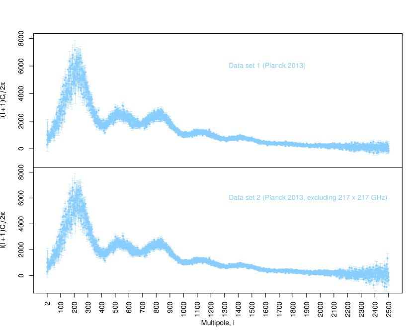
Figure 1: The weighted-average Planck 2013 temperature angular power spectrum data. Data set 1, is the weighted-average of the background CMB angular power spectra from combination of $100\times 100$ GHz, $143\times 143$ GHz, $217\times 217$ GHz and $143\times 217$ GHz spectra at ($\ell\geq 50$). Data set 2, is similar to data set 1, except that the angular power spectrum of $217\times 217$ GHz is excluded. The angular power spectrum at $\ell<50$ in both data sets is given by Planck team and obtained by using the Planck frequency channels from 30 to 353 GHz [6].

3 Methodology

The REACT is a nonparametric function estimation and was initially proposed by [17, 18, 19, 20] and then modified and used in CMB data analysis by [21, 22, 13, 23, 14].

The function estimation or regression methods estimate the unknown function $f$, related to given data set, by using the estimate $\widehat{f}$. The nonparametric function estimation methodologies do not assume a specific functional form for $f$ and attempt to estimate the function with some mild regularity assumptions such as smoothness or membership of $f$ to a function space, etc. In REACT formalism an estimate $\widehat{f}$ of unknown function $f$ is obtained by balancing bias and variance of $\widehat{f}$ through optimal smoothing which is achieved by minimizing the risk function. This nonparametric methodology also constructs a confidence set around the $\widehat{f}$ which can be employed in many aspects of inference.

In this section we first present a review of this methodology (Subsections 3.1 and 3.2) which is mainly based on [21, 22, 13]. Our calibration of confidence distances based on the Monte Carlo simulations in order to test the consistency of an assumed cosmological model with observation, is presented in Subsection 3.3. In addition we describe (Subsection 3.4) a way of bias estimation of $\widehat{f}$ based on the Monte Carlo simulations to demonstrate the consistency in multipole space.

3.1 The nonparametric fit and confidence set

The CMB angular power spectrum data is given in the form of

$$Y_{\ell}={\cal D}_{\ell}+\epsilon_{\ell}$$ (3.1)

where $Y_{\ell}$ repersents the $N$ observed data points over multipoles equal to true but unknown angular power spectrum ${\cal D}_{\ell}\equiv f(x_{\ell})$ contaminated with the noise, $\epsilon_{l}$, which is assumed to have normal distribution with mean-0 and known covariance matrix $\Sigma$.

The main assumption in REACT formalism is that the unknown function $f$, belongs to $L_{2}$ function space, such as it can be expanded in a complete orthonormal basis $\{\phi_{j}(x)\}$,

$$f(x)=\sum_{j=0}^{\infty}\beta_{j}\phi_{j}(x).$$

A proven useful basis for the CMB angular power spectrum estimation is the cosine basis defined over $0\leq x\leq 1$:

$$\phi_{j}(x)=\begin{cases}1\;\;\;\;\;\;\;\;\;\;\;\;\;\;\;\;\;\;(j=0)\\ \sqrt{2}\cos(j\pi x)\;(j=1,2,\ldots)\end{cases}.$$ (3.2)

Assuming $f$ is sufficiently smooth and considering $N$ data points, we can take

$$f(x)\approx\sum_{j=0}^{N-1}\beta_{j}\phi_{j}(x),$$

and estimate it as

$$\widehat{f}(x)=\sum_{j=0}^{N-1}\widehat{\beta}_{j}\phi_{j}(x).$$ (3.3)

The angular power spectrum ${\cal D}_{\ell}\equiv f(x_{\ell})$ would be estimated as $\widehat{{\cal D}}_{\ell}\equiv\widehat{f}(x_{\ell})$ through coefficient estimates $\widehat{\beta}_{j}$ which are estimated as

$$\widehat{\beta}_{j}=\lambda_{j}Z_{j},$$ (3.4)

where

$$Z_{j}={1\over N}\sum_{i=0}^{N-1}Y_{i}\phi_{j}(x_{i})={(U^{T}Y)_{j}\over\sqrt{N}}.$$ (3.5)

Here, $U$ is the orthonormal matrix defined as $U_{ij}=\phi_{j}(x_{i})/\sqrt{N}$ and $Y\equiv(Y_{0},\ldots,Y_{N-1})^{T}$

Finding the coefficient estimates $\widehat{\beta}\equiv(\widehat{\beta}_{0},\ldots,\widehat{\beta}_{N-1})^{T}$, and hence the $\widehat{f}(x)$, could be reduced to determining the shrinkage parameters $\lambda_{j}$. The smoothness assumption of $f$ implies a fast decay of the true coefficients $\beta_{j}$ with $j$. This suggests a monotonically decreasing constraint on shrinkage parameters

$$1\geq\lambda_{0}\geq\lambda_{1}\geq\ldots\geq\lambda_{N-1}\geq 0\;\;\mbox{(Monotone shrinkage)}.$$ (3.6)

Using shrinkage parameters one can define the effective degree of freedom (EDoF) as

$$\mbox{EDoF}(\lambda)=\sum_{j=0}^{N-1}\lambda_{j}.$$ (3.7)

Effective degree of freedom can be used to characterize the nonparametric function estimation $\widehat{f}(x)$ and interpreted as the degree of smoothness.

In this formalism the difference between the true unknown function $f(x)$ and its estimator $\widehat{f}(x)$ is measured via the inverse-noise-weighted loss function $L(\lambda)$,

$$L(\lambda)=\int_{0}^{1}\left({f(x)-\widehat{f}(x)\over\sigma(x)}\right)^{2}dx.$$ (3.8)

where $\sigma^{2}(x)$ is the variance of the data $Y$ and $\lambda\equiv(\lambda_{0},\ldots,\lambda_{N-1})^{T}$ is the vector of shrinkage parameters.

Optimal smoothing is obtained by balancing the bias of the function estimator $\widehat{f}(x)$ with its variance, by minimizing the risk function $R(\lambda)$, which is the expected value of loss function $L(\lambda)$,

$$R(\lambda)=\int_{0}^{1}\left({f(x)-\mathbb{E}\left(\widehat{f}(x)\right)\over\sigma(x)}\right)^{2}dx+\int_{0}^{1}\mathbb{E}\left[\left({\widehat{f}(x)-\mathbb{E}\left(\widehat{f}(x)\right)\over\sigma(x)}\right)^{2}\right]dx.$$

Where the two terms are the integrated squared bias and the integrated variance of function estimator $\widehat{f}(x)$, both weighed by $1/\sigma^{2}(x)$.

Since the risk function $R(\lambda)$ depends on the unknown function $f$, it needs to be estimated through an estimator. A particular Stein’s Unbiased Risk Estimator (SURE) [24] of this risk take the following form

$$\widehat{R}(\lambda)=Z^{T}\bar{D}W\bar{D}Z+\mbox{tr}(DWDB)-\mbox{tr}(\bar{D}W\bar{D}B)$$ (3.9)

where $D\equiv\mbox{diag}(\lambda_{0},\ldots,\lambda_{N-1})$, $\bar{D}=I_{N}-D$, $Z\equiv(Z_{0},\ldots,Z_{N-1})^{T}$, $B=U^{T}\Sigma U/N$ is the covariance of $Z$, and $I_{N}$ is the $N\times N$ identity matrix. Using approximate expansion $(1/\sigma^{2}(x))\approx\sum_{j=0}^{N-1}w_{j}\phi_{j}(x)$, the weight matrix $W$ would be defined as

$$W_{jk}=\sum_{l}\Delta_{jkl}w_{l},$$ (3.10)

where,

$$\Delta_{jkl}=\int_{0}^{1}\phi_{j}(x)\phi_{k}(x)\phi_{l}(x)\hskip 2.84526ptdx=\left\{\begin{array}[]{ll}1,&\mbox{if }\#\{j,k,l=0\}=3,\\ 0,&\mbox{if }\#\{j,k,l=0\}=2,\\ \delta_{jk}\delta_{0l}+\delta_{jl}\delta_{0k}+\delta_{kl}\delta_{0j},&\mbox{if }\#\{j,k,l=0\}=1,\\ \frac{1}{\sqrt{2}}(\delta_{l,j+k}+\delta_{l,|j-k|})&\mbox{if }\#\{j,k,l=0\}=0.\\ \end{array}\right.$$

for the cosine basis (Eq. 3.2).

We have already mentioned the optimal nonparametric fit obtained by minimizing risk $\widehat{R}(\lambda)$ by $\widehat{\lambda}$ and through Equations 3.3 & 3.4. The estimated fit is the nonparametric fit without any restriction on its EDoF which is called the full-freedom fit. This full-freedom fit in CMB data analysis can be quite wiggly in some multipoles where the noise levels in the data is high. While this full-freedom fit is a reasonable reconstruction (in a sense that it captures the essential trends in the data), most cosmological models predicts smooth forms of the angular power spectrum. Alternatively, imposing additional constraint of the form

$$\sum_{i=0}^{N-1}\lambda_{i}=q,$$ (3.11)

where $q$ constrains the EDoF of the fit, leads to the smoother restricted-freedom fit. By gradually reducing the value of EDoF (relative to the full-freedom fit) we can obtain an acceptably smooth fit.

Conventional curve estimation methods provide a confidence band around the best fit that indicates the uncertainty in the reconstruction. Instead, this nonparametric methodology quantifies the uncertainty surrounding the nonparametric fit in the form of a high-dimensional $(1-\alpha)$ confidence set (confidence ball) at a pre-specified $0\leq(1-\alpha)\leq 1$ confidence level. By definition the confidence ball asymptotically contains the true model with probability equal to associated confidence level. This confidence set for coefficient vector $\beta$ is centered at $\widehat{\beta}$ and is defined as

$$\mathcal{S}_{N,\alpha}=\left\{\beta:(\beta-\widehat{\beta})^{T}W(\beta-\widehat{\beta})\leq{r}^{2}_{\alpha}\right\},$$ (3.12)

where the confidence radius ${r}_{\alpha}$ is calculated by

$${r}^{2}_{\alpha}={\widehat{\tau}z_{\alpha}\over\sqrt{N}}+\widehat{R}(\widehat{\lambda}).$$ (3.13)

Here $z_{\alpha}$ is upper $\alpha$ quantile of standard normal distribution, and

$$\widehat{\tau}^{2}/N=2\mbox{tr}(ABAB)+Z^{T}QZ-\mbox{tr}(QB),$$ (3.14)

where $Q=4(ABA+WDBDW-2ABDW)$ and $A=DW+WD-W$.

On the other hand, loss function (Equation 3.8) can be written approximately for $N$ data points as

$$L(\lambda) \approx {1\over N}\sum_{\ell=\ell_{min}}^{\ell_{max}}\left(f(x_{\ell})-\widehat{f}(x_{\ell})\over\sigma(x_{\ell})\right)^{2}$$ (3.15)

$$\approx (\beta-\widehat{\beta})^{T}W(\beta-\widehat{\beta})$$ (3.16)

Consequently the high-dimensional confidence set around the $\widehat{\beta}$ (Equation 3.12) can be interpreted as a confidence ball in a high-dimensional function space with the center of nonparametric fit $\widehat{f}$ weighed by $1/\sigma^{2}(x_{\ell})$, with the same confidence radius ${r}_{\alpha}$ (Equation 3.13) to $(1-\alpha)$ pre-specified confidence level. Apart from the main application of confidence ball which is determining the uncertainties on the nonparametric fit and associated features, we can employ this for validating different cosmological models in a model-independent way. We will discuss this in the next subsection.

3.2 Validating cosmological models

Basically the high-dimensional confidence ball, centered in the nonparametric fit, determines the uncertainties around the fit. Furthermore we can use this concept for validating different cosmological models against the data model-independently. In this regard we measure the distance $d$ of the point associated to a predicted angular power spectrum of a specific cosmological model to the center of the confidence ball. Using Equation 3.15 the distance, $d$, would be

$$d=\sqrt{{1\over N}\sum_{\ell=\ell_{min}}^{\ell_{max}}\left({\cal D}^{model}_{\ell}-\widehat{{\cal D}}_{\ell}\over\sigma_{\ell}\right)^{2}}.$$ (3.17)

where $\widehat{{\cal D}}_{\ell}$ and ${\cal D}^{model}_{\ell}$ are nonparametric and predicted angular power spectrum in each $\ell$ respectively. The $\sigma^{2}_{\ell}$ is the variance of angular power spectrum data in each $\ell$ and $N$ is the total number of multipoles. This distance can be associated to the confidence level that a proposed angular power spectrum can be rejected as a candidate for the true model (confidence distance). For this purpose if we rearrange the Equation 3.13, the upper $\alpha$ quantile of standard normal distribution $z_{\alpha}(d)$, associated with distance $d$ would be

$$z_{\alpha}(d)=\frac{\sqrt{N}}{\widehat{\tau}}\left(d^{2}-\widehat{R}(\widehat{\lambda})\right)$$ (3.18)

By definition the cumulative distribution function of the standard normal distribution of $z_{\alpha}(d)$ represents confidence distance (associated confidence level with particular distance $d$). In other words through this procedure we can measure the consistency of a specific cosmological model with the data in a model-independent way.

3.3 Calibrating confidence distances

Although the original formalism in REACT provides an elegant procedure to assign a confidence level to a particular distance from the center of nonparametric confidence set. However, in this procedure the calculated confidence level is highly dependent on the minimum risk value of the nonparametric fit (Equation 3.18) which is based on a single data realization and REACT is usually very conservative in estimation of inconsistencies between data sets and models. To address this issue and in order to have a more accurate estimation of the level of consistency (or inconsistency) between the concordance model of cosmology and Planck 2013 data we perform a calibration based on many simulated realizations of the angular power spectrum data, ${\cal D}^{sim}_{\ell}$. Since the main goal is to check the consistency of the Planck best fit $\Lambda$CDM model with data, we assume the Planck best fit $\Lambda$CDM as the true model and add the Gaussian noise according to the calculated covariance matrix in Equation 2.2. Next we estimate the full-freedom fit, $\widehat{{\cal D}}^{sim}_{\ell}$, of each simulated angular power spectrum data.

Using Equation 3.17, the distance of the Planck best fit $\Lambda$CDM (true model) and the full-freedom fit, $\widehat{{\cal D}}^{sim}_{\ell}$, of each simulated angular power spectrum data, can be calculated. The empirical Cumulative Distribution Function (CDF) of these distances can be used as the calibrated confidence level of distances (calibrated confidence distances). Statistically, the obtained CDF indicates the probability of existence of true model in distance of shorter or equal to a specific distance in function space. In fact these calibrated confidence distances present the (calibrated) confidence levels associated to distances from nonparametric fit in function space. We demonstrate these results in Section 4.

It is worth noting that while the nonparametric fit obtained by minimizing the risk estimator $\widehat{R}(\lambda)$ depends on the full covariance matrix of data $\Sigma$ (Equation 3.9), the distance $d$ (Equation 3.17) which is derived from the loss function uses only the diagonal terms of $\Sigma$. This would not affect the reliability of the final results since we have used Monte Carlo simulations and treated the real and simulated data in a same way. However, the method may become more sensitive to possible features in the angular power spectrum if the full covariance matrix in defining distances is employed.

3.4 Bias control

In Subsection 3.1 we see the nonparametric fit is estimated by minimizing the risk function that results to an optimally smooth reconstruction. In principle, too much of smoothing leads to a fit with high bias and low variance, and too little smoothing yields a fit with low bias and high variance. Minimal risk (optimal smoothing) therefore can be thought then as a reconstruction with a balance between the bias and the variance. Therefore the nonparametric fit in this formalism has an optimal smoothing with the cost of some bias.

Using the simulations we mentioned earlier, we are able to estimate the bias and make our reconstructions more accurate. In this procedure we use the distribution of the full-freedom fits, $\widehat{{\cal D}}^{sim}_{\ell}$, in each $\ell$ obtained from our simulated angular power spectrum data to find out the form of the bias. The median of the distribution of $\widehat{{\cal D}}^{sim}_{\ell}$ in each $\ell$ represents an estimated angular power spectrum, $\widehat{{\cal D}}^{med}_{\ell}$, which tends to show true angular power spectrum, ${\cal D}^{true}_{\ell}$. Therefore the bias can be estimated as

$$\text{bias}(\ell)=\widehat{{\cal D}}^{med}_{\ell}-{\cal D}^{true}_{\ell}$$ (3.19)

Then the calibrated unbiased nonparametric fit, $\widehat{{\cal D}}^{unb}_{\ell}$, is obtained by subtracting the bias at each $\ell$ from the nonparametric fit, $\widehat{{\cal D}}_{\ell}$,

$$\widehat{{\cal D}}^{unb}_{\ell}=\widehat{{\cal D}}_{\ell}-\text{bias}(\ell)$$ (3.20)

The residual of Planck best fit $\Lambda$CDM and unbiased nonparametric fit can be calculated as

$$\text{Res}(\ell)={\cal D}^{\Lambda CDM}_{\ell}-\widehat{{\cal D}}^{unb}_{\ell}$$ (3.21)

where $\text{Res}(\ell)$ is the residual value at each $\ell$ and the ${\cal D}^{\Lambda CDM}_{\ell}$ is the Planck best fit $\Lambda$CDM. Since we assume the best fit $\Lambda$CDM as the true model in simulation procedure (Subsection 3.3), then ${\cal D}^{true}_{\ell}={\cal D}^{\Lambda CDM}_{\ell}$. Therefore from Equations 3.19, 3.20 and 3.21, the residual equation would be simplified to

$$\text{Res}(\ell)=\widehat{{\cal D}}^{med}_{\ell}-\widehat{{\cal D}}_{\ell}$$ (3.22)

The residual, $\text{Res}(\ell)$, represents the deviation of the Planck best fit $\Lambda$CDM model from Planck 2013 data in different multipole ranges estimated by the unbiased nonparametric reconstruction, $\widehat{{\cal D}}^{unb}_{\ell}$.

In addition, the uncertainties of unbiased nonparametric fit, $\widehat{{\cal D}}^{unb}_{\ell}$ can be estimated by simulations. Using the distribution of the full-freedom fits, $\widehat{{\cal D}}^{sim}_{\ell}$, in each $\ell$, we can estimate the corresponding $1$ and $2\sigma$ error bars around $\widehat{{\cal D}}^{med}_{\ell}$. These uncertainties would be propagated identically to $\widehat{{\cal D}}^{unb}_{\ell}$, in each $\ell$, through Equations 3.19 & 3.20. They can be used to quantify the deviation of the Planck best fit $\Lambda$CDM model from the unbiased nonparametric reconstruction in terms of confidence levels.

4 Results

The full-freedom fit and the restricted-freedom fit of data set 1 (full Planck 2013 data) correspond to EDoF $\sim 130$ and EDoF $=25$ respectively. Figure 2 (top panel) shows the full-freedom fit and the restricted-freedom fit of data set 1 with green and red points. Applying the same nonparametric methodology (described in Subsection 3.1) on data set 2 (Planck 2013 data excluding $217\times 217$ GHz) we achieve the full-freedom fit at EDoF $\sim 106$ and the restricted-freedom fit at EDoF $=26$. The full-freedom fits (Figures 2 and 3, green points) turn out to be a little wiggly most likely due to the noise in the corresponding data set. Rather, the restricted-freedom fits (Figures 2 and 3, red points) exhibit a smooth angular power spectrum with $6$ peaks up to $\ell\sim 2000$ as expected in the standard cosmology. We see for both sets of data, the restricted-freedom fits follow the corresponding full-freedom fits closely. For comparison we also plot the Planck best fit $\Lambda$CDM (Figures 2 and 3, black points). We see all three fits by and large follow the same trend except for small deviations. In particular, the best fit $\Lambda$CDM model shows an up-turn at $\ell<10$ which we expect to see in the concordance model of cosmology due to the integrated Sachs-Wolfe effect [25]. However, neither the restricted-freedom nonparametric fits nor the full-freedom fits, reveal such an upturn.

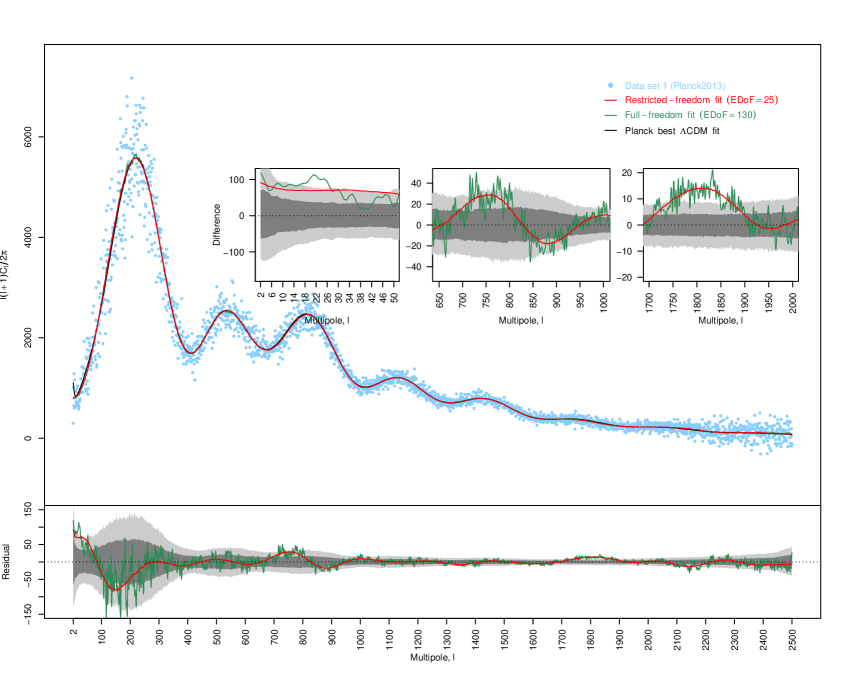
Figure 2: (Top panel) The nonparametric fits for Planck 2013 temperature angular power spectrum data (data set 1). Green: full-freedom fit (EDoF $\sim 130$), red: restricted-freedom fit (EDoF $=25$), black: best fit $\Lambda$CDM model, blue: data set 1, Planck 2013 angular power spectrum data. The bottom panel illustrates the residuals of the best fit $\Lambda$CDM model with respect to unbiased nonparametric fits. The $1\sigma$ and $2\sigma$ confidence bands are plotted in dark and light gray colors. Results show the deviation of the best fit $\Lambda$CDM model from data in three multipole ranges (highlighted in top panel inset plots). These deviations are at low multipoles $18<\ell<26$ with greater than $2\sigma$ significance, $\ell\sim 750$ at $1$ to $\sim 2\sigma$ significance and $\ell\sim 1800$ at greater than $2\sigma$ significance.

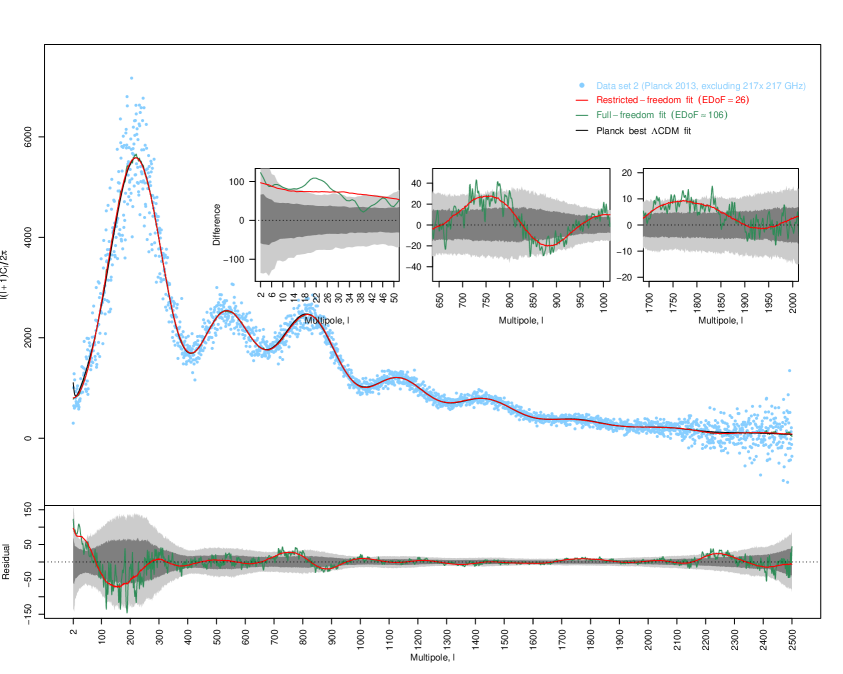
Figure 3: (Top panel) The nonparametric fits for Planck 2013 temperature angular power spectrum data excluding $217\times 217$ GHz spectrum (data set 2). Green: full-freedom fit (EDoF $\sim 106$), red: restricted-freedom fit (EDoF $=26$), black: best fit $\Lambda$CDM model, blue: data set 2, Planck angular power spectrum data (excluding $217\times 217$ GHz power spectrum). The bottom panel illustrates the residuals of the best fit $\Lambda$CDM model with respect to unbiased nonparametric fits. The $1\sigma$ and $2\sigma$ confidence bands are plotted in dark and light gray colors respectively. The residual of unbiased full-freedom fit (green curve) and unbiased restricted-freedom fit (red curve) show the deviation of the best fit $\Lambda$CDM model from data in three multipole ranges (highlighted in top panel inset plots). They show the deviations at low multipoles $18<\ell<26$ with greater than $2\sigma$ significance, $\ell\sim 750$ at $1$ to $\sim 2\sigma$ significance and $\ell\sim 1800$ at $1$ to $\sim 2\sigma$ significance. The significance of the feature at $\ell\sim 1800$ is reduced considerably by excluding the $217\times 217$ GHz spectrum from the Planck 2013 data.

For testing the consistency of the Planck best fit $\Lambda$CDM and the data we employ the Monte Carlo simulation described in Subsection 3.3. The simulations mimic 1000 independent observations of angular power spectrum for data set 1 and 2 all based on the best fit $\Lambda$CDM model. Applying the nonparametric method we obtain the full-freedom fits of the simulated data and the corresponding distances to the Planck best fit $\Lambda$CDM (as the true model). The estimated Probability Density Functions (PDF) of the calculated distances are shown for data set 1 and data set 2, in Figure 4, top-left and top-right panels respectively. Furthermore the corresponding empirical Cumulative Distribution Functions (CDF) are plotted in Figure 4 (bottom panels). These plots will provide us a scale that at what distances the best fit $\Lambda$CDM model and the full-freedom non-parametric fits should stand if the observed data is a true realization of the concordance model.

Using the Equation 3.17, the Planck best fit $\Lambda$CDM stands in function space at the distances $1.172\times 10^{-1}$ and $9.932\times 10^{-2}$ to the full-freedom fits associated with data set 1 and data set 2 respectively. Locating these numbers in the CDF diagrams of the data set 1 and 2 (Figure 4, bottom panels) we find that the corresponding confidence levels of these distances are $0.95$ and $0.70$ respectively.

Deriving the confidence levels, we also attempt to transfer these information from the function space to multipole $\ell$ angular power spectrum space. As described in Subsection 3.4, we try to remove the bias from the nonparametric fits in order to compare them with the best fit $\Lambda$CDM model. We use distribution of 1000 full-freedom fits at each $\ell$ obtained from the simulated angular power spectrum data (which are all based on the best fit $\Lambda$CDM model) and calculate the median values, $\widehat{{\cal D}}^{med}_{\ell}$. We use these median values at each $\ell$ to derive residuals through Equation 3.22. Figures 2 and 3 (bottom panels) illustrate the residual values of the best fit $\Lambda$CDM model with respect to the (unbiased) full-freedom fit (green curve) using data set 1 and data set 2 respectively. The median, $\widehat{{\cal D}}^{med}_{\ell}$ is indicated as the zero line (black dotted line) in these plots. The $1\sigma$ and $2\sigma$ confidence bands based on the simulations are shown by dark and light gray colors. We should note here that since in Figures 2 and 3 (bottom panels) we plot the residuals of the best fit $\Lambda$CDM model with respect to the nonparametric fit the zero line represents the nonparametric fit. From Figure 2 (bottom panel) we see that the most prominent deviations between the nonparametric reconstructions and the best fit $\Lambda$CDM model seems to be at low multipoles $18<\ell<26$ at greater than $2\sigma$ significance, $\ell\sim 750$ at $1$ to $\sim 2\sigma$ significance and $\ell\sim 1800$ at greater than $2\sigma$ significance. For better illustration these three regions are replotted in top panel, inset plots. Figure 2 (bottom panel) shows the similar plots for data set 2 (Planck 2013 excluding $217\times 217$ GHz spectrum). We see that the feature at $\ell\sim 1800$ becomes substantially less significant at $1$ to $\sim 2\sigma$ confidence level. Considering all these, the deviations at low multipoles and $\ell\sim 750$ looks to be the most prominent feature in the Planck 2013 data.

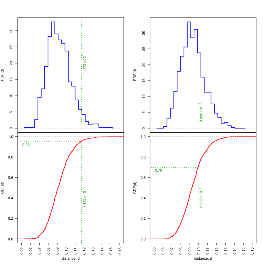
Figure 4: The estimated Probability Density Functions (PDF) of the distance parameter, $d$, (Equation 3.17) from 1000 simulations of the Planck 2013 data (based on the best fit $\Lambda$CDM model) for data set 1 (top-left panel) and data set 2 (top-right panel). The bottom panels shows the empirical Cumulative Distribution Function (CDF) corresponding to PDF of data set 1 (left-bottom panel) and data set 2 (right-bottom panel). In comparison and in the case of the actual real data, the Planck 2013 best fit $\Lambda$CDM stands at $1.172\times 10^{-1}$ distance (left-bottom panel, green vertical dotted line) from the corresponding full-freedom fit in the function space. This can be interpreted that the best fit $\Lambda$CDM model is consistent to the Planck 2013 data at $95\%(\sim 2\sigma)$ confidence level (left-bottom panel, green horizontal dotted line). Excluding the $217\times 217$ GHz spectrum (data set 2), the Planck best fit $\Lambda$CDM stands in $9.932\times 10^{-2}$ distance (right-bottom panel, green vertical dotted line) with respect to the corresponding full-freedom fit in the function space which make this model to be consistent to the data set 2 (Planck 2013 excluding $217\times 217$ GHz spectrum) at $70\%(\sim 1\sigma)$ confidence level (right-bottom panel, green horizontal dotted line).

5 Conclusion

In this paper we have calibrated REACT confidence distances to present an algorithm to accurately estimate the consistency of an assumed theoretical cosmological model with CMB data. Using our nonparametric method we reconstruct the form of the angular power spectrum from the data and compare our results with the theoretically expected angular power spectrum. We recently performed an analysis of comparing the best fit $\Lambda$CDM model and Planck data using REACT in [14] where we have calculated the confidence distance of the standard $\Lambda$CDM model from the center of the nonparametric confidence set.

However, in this work in order to have a more accurate quantitative statistical measure of comparison between the nonparmetric results and the model theoretical expectations we calibrated our consistency measure using many realizations of the data all based on the same theoretical model. While the actual REACT is very conservative in estimation of the inconsistencies between data sets and models and we found previously that the best fit $\Lambda$CDM model is at $36\%(\sim 0.5\sigma)$ confidence distance from the center of the nonparametric confidence set using Planck 2013 temperature data, our calibrated results put the best fit $\Lambda$CDM model at $95\%(\sim 2\sigma)$ confidence distance from the center of the nonparametric confidence set. In this work we have simulated 1000 Monte Carlo realizations of the Planck 2013 temperature angular power spectrum data based on the best fit $\Lambda$CDM model and for each realization we derived the confidence distance between the best nonparametric fit and the true model. We used the distribution of these confidence distances from the simulations to calibrate REACT in this particular problem and we compared the derived distribution with the results from the actual data. Our results indicate that the distance between the best fit $\Lambda$CDM model from the center of the nonparametric confidence set in the case of the real Planck 2013 temperature data is larger than the similar distances we derived in simulations in $95\%$ of the cases. Our results seems to be in a very close agreement with some other analysis discussing the same subject using different methodologies  [11, 10, 12]. Excluding the 217 GHz data from our analysis, the best fit $\Lambda$CDM model shifts to $70\%(\sim 1\sigma)$ confidence distance from the center of nonparametric confidence set resulting to better consistency of the standard model with Planck data. While the $217\times 217$ spectrum is one of the most precise CMB measurements of the Planck, in [15] it has been mentioned that there has been a small systematic in this frequency channel (apparently due to incomplete removal of 4 K cooler lines). This probably can be a reason behind the significant inconsistency we derived between the standard $\Lambda$CDM model and full Planck 2013 data. Excluding the $217\times 217$ spectrum from our analysis and getting significantly better consistency between Planck 2013 and the concordance model seems to support this argument. However, repetition of the analysis using Planck 2015 can make things much more clear.

Using this algorithm we can also highlight the angular scales where the assumed theoretical model deviates from the data (with considerable statistical significance) using large number of simulations and after some bias control. We should recall that REACT and consequently our calibrated REACT in this analysis is a biased estimator and while this would not affect our consistency test, to look for angular scales deviating from the concordance model we should perform a bias control. We can perform this bias control using extensive simulations and subsequently correct/modify the estimated forms of the angular power spectrum. Applying our approach on Planck temperature 2013 data and assuming the best fit spatially flat $\Lambda$CDM model, after performing the bias control and error-estimation our results indicate that the most prominent features in the Planck 2013 data deviating from the best fit $\Lambda$CDM model seems to be at low multipoles $18<\ell<26$ with greater than $2\sigma$ significance, $\ell\sim 750$ at $1$ to $\sim 2\sigma$ significance and $\ell\sim 1800$ with greater than $2\sigma$ significance. Excluding the 217 GHz data the feature at $\ell\sim 1800$ becomes substantially less significant at $1$ to $\sim 2\sigma$. While the feature at $\ell\sim 1800$ seems to be due to some systematics in the data, the features at $\ell\sim 750$ looks to be the most prominent feature in the Planck 2013 data. Similar results have been reported earlier using alternative methods [26].

To summarize, in this paper we propose an approach based on calibration of REACT confidence distances where we can test the consistency of a particular theoretical model with CMB observations and also look for the multipole scales where there are significant deviations. We have applied the method on Planck 2013 data in order to show its strength and simplicity and it can be trivially used against forthcoming data including Planck 2015.

References

- [1] C. L. Bennett et al. Nine-year Wilkinson Microwave Anisotropy Probe (WMAP) Observations: Final Maps and Results, Astrophys. J. Supplement 208 (Oct., 2013) 20, [arXiv:1212.5225].
- [2] G. Hinshaw et al. Nine-year Wilkinson Microwave Anisotropy Probe (WMAP) Observations: Cosmological Parameter Results, Astrophys. J. Supplement 208 (Oct., 2013) 19, [arXiv:1212.5226].
- [3] P. A. R. Ade et al. Planck 2013 results. I. overview of products and scientific results, A&A 571 (2014) A1.
- [4] J. L. Sievers et al. The Atacama Cosmology Telescope: cosmological parameters from three seasons of data, J. Cosmology Astropart. Phys. 10 (Oct., 2013) 60, [arXiv:1301.0824].
- [5] K. T. Story et al. A Measurement of the Cosmic Microwave Background Damping Tail from the 2500-Square-Degree SPT-SZ Survey, Astrophys. J. 779 (Dec., 2013) 86, [arXiv:1210.7231].
- [6] P. A. R. Ade et al. Planck 2013 results. XV. cmb power spectra and likelihood, A&A 571 (2014) A15.
- [7] P. A. R. Ade et al. Planck 2013 results. XVI. cosmological parameters, A&A 571 (2014) A16.
- [8] P. A. R. Ade et al. Planck 2013 results. XXXI. consistency of the planck data, A&A 571 (2014) A31.
- [9] A. Kovács, J. Carron, and I. Szapudi, On the coherence of WMAP and Planck temperature maps, Mon.Not.Roy.Astron.Soc 436 (Dec., 2013) 1422–1429, [arXiv:1307.1111].
- [10] D. K. Hazra and A. Shafieloo, Test of consistency between Planck and WMAP, Phys. Rev. D 89 (Feb., 2014) 043004, [arXiv:1308.2911].
- [11] D. K. Hazra and A. Shafieloo, Confronting the concordance model of cosmology with Planck data, Journal of Cosmology and Astroparticle Physics 1 (Jan., 2014) 43, [arXiv:1401.0595].
- [12] D. Larson, J. L. Weiland, G. Hinshaw, and C. L. Bennett, Comparing Planck and WMAP: Maps, Spectra, and Parameters, ArXiv e-prints (Sept., 2014) [arXiv:1409.7718].
- [13] A. Aghamousa, M. Arjunwadkar, and T. Souradeep, Evolution of the cosmic microwave background power spectrum across wilkinson microwave anisotropy probe data releases: A nonparametric analysis, Astrophys. J. 745 (2012), no. 2 114.
- [14] A. Aghamousa, A. Shafieloo, M. Arjunwadkar, and T. Souradeep, Unveiling acoustic physics of the cmb using nonparametric estimation of the temperature angular power spectrum for planck, Journal of Cosmology and Astroparticle Physics 2015 (2015), no. 02 007.
- [15] P. A. R. Ade et al. Planck 2013 results. XXII. constraints on inflation, A&A 571 (2014) A22.
- [16] D. Spergel, R. Flauger, and R. Hlozek, Planck Data Reconsidered, ArXiv e-prints (Dec., 2013) [arXiv:1312.3313].
- [17] R. Beran, Confidence sets centred at -estimators, Ann. Inst. Statist. Math. 48 (1996) 1–15.
- [18] R. Beran and L. Dümbgen, Modulation of estimators and confidence sets, Ann. Statist. 26 (1998), no. 5 1826–1856.
- [19] R. Beran, React scatterplot smoothers: Superefficiency through basis economy, J. Amer. Statist. Assoc. 95 (2000), no. 449 155–171.
- [20] R. Beran, React trend estimation in correlated noise, in Asymptotics in statistics and probability: papers in honor of George Gregory Roussas (M. L. Puri, ed.), pp. 1–16. VSP International Science Publishers, 2000.
- [21] C. R. Genovese, C. J. Miller, R. C. Nichol, M. Arjunwadkar, and L. Wasserman, Nonparametric inference for the cosmic microwave background, Statist. Sci. 19 (2004), no. 2 308–321.
- [22] B. Bryan, J. Schneider, C. J. Miller, R. C. Nichol, C. R. Genovese, and L. Wasserman, Mapping the cosmological confidence ball surface, Astrophys. J. 665 (August, 2007) 25–41.
- [23] A. Aghamousa, M. Arjunwadkar, and T. Souradeep, Model-independent forecasts of cmb angular power spectra for the planck mission, Phys. Rev. D 89 (Jan, 2014) 023509.
- [24] C. M. Stein, Estimation of the mean of a multivariate normal distribution, The Annals of Statistics 9 (1981), no. 6 1135–1151.
- [25] R. K. Sachs and A. M. Wolfe, Perturbations of a Cosmological Model and Angular Variations of the Microwave Background, Astrophys. J. 147 (Jan., 1967) 73.
- [26] D. K. Hazra, A. Shafieloo, and T. Souradeep, Primordial power spectrum from Planck, Journal of Cosmology and Astroparticle Physics 11 (Nov., 2014) 11, [arXiv:1406.4827].
- [27] R Core Team, R: A Language and Environment for Statistical Computing. R Foundation for Statistical Computing, Vienna, Austria, 2013.