Varieties via their L-functions

Abstract.

We describe a procedure for determining the existence, or non-existence, of an algebraic variety of a given conductor via an analytic calculation involving L-functions. The procedure assumes that the Hasse-Weil L-function of the variety satisfies its conjectured functional equation, with no assumption of an associated automorphic object or Galois representation. We demonstrate the method by finding the Hasse-Weil L-functions of all hyperelliptic curves of conductor less than 500.

1. Introduction

Many objects in number theory are associated to L-functions. Familiar examples include modular forms, Galois representations, and algebraic varieties. One might think of those as the fundamental objects, and the associated L-function as a shadow that serves as a placeholder for some of the invariants of the object. For example, the L-function of an elliptic curve contains information about the conductor of the curve and the number of points on the curve $\text{mod }p$, for each prime $p$. But the L-function does not know everything about the curve. For example, it does not know how many torsion points are on the curve: it only has information about a particular combination of the torsion order, regulator, and a few other parameters as described in the formula of Birch and Swinnerton-Dyer. Of course, this apparent shortcoming is due to the fact that the translation from an elliptic curve to its L-function goes via the Jacobian, and the Jacobian only sees the isogeny class of the curve. As far as we know, no information is lost when translating from the Jacobian/isogeny class to the L-function.

While it has been natural to view L-functions as arising from other objects, in this paper we make the point that it is possible to detect the L-function without having access to the associated object. By “detect” we mean that one can find the Dirichlet coefficients and functional equation parameters in a practical manner involving a computer calculation. We have demonstrated this principle for L-functions of Maass forms on $\mathrm{GL}(3)$, $\mathrm{GL}(4)$, and ${\rm Sp}(4)$, see [6]. There are many internal consistency checks for those calculations, but in most cases there does not currently exist an independent method to generate the data for the underlying Maass form. In the present paper, the L-functions we consider are associated to several types of arithmetic objects, as described in Section 2.3. In most cases this allows for independent verification of our calculations.

In the next section, we describe the L-functions  we will consider, we list (some of) the associated objects, and we summarize the results of our calculations. Details of our method are given in the following sections.

2. Axioms for L-functions

This paper takes an axiomatic approach to L-functions. The most famous example of this approach is the Selberg class [17]. Selberg’s axioms are as general as possible: all known (or conjectured) L-functions satisfy much stricter conditions. Since our methods involve computer calculations, we seek axioms that are as restrictive as possible. This reduces the size of the space we must search.

A proposal for such a set of axioms is given in [7]. We specialize to the case of “tempered arithmetic entire L-functions of degree 4, weight 1, and trivial central character, which have rational integer coefficients in the arithmetic normalization.” While that set of L-functions may appear highly specialized, there are many objects which give rise to such L-functions, for example a hyperelliptic curve $C/{\mathbb{Q}}$ of genus 2 or an abelian surface $A/{\mathbb{Q}}$. See Section 2.3 for more examples.

2.1. The Axioms

Below is a complete list of the properties we assume for the L-functions in our search.

Dirichlet series:

$$L(s)=\sum_{n=1}^{\infty}\frac{A_{n}/\sqrt{n}}{n^{s}},\ \ \ \ \ \ \ \ \ \ \ \ \ \ \ A_{n}\in{\mathbb{Z}},$$ (2.1)

with $A_{n}\ll n^{\frac{1}{2}+\varepsilon}$.

Functional equation:

$$\Lambda(s):=N^{s/2}\ \Gamma_{\mathbb{C}}(s+\tfrac{1}{2})^{2}\,L(s),$$ (2.2)

originally defined by (2.1) for $s=\sigma+it$ with $\sigma>1$, continues to an entire function which satisfies the functional equation

$$\Lambda(s)\,=\,\varepsilon\,\Lambda(1-s),$$ (2.3)

where $\varepsilon=\pm 1$. The positive integer $N$ is called the conductor of the L-function, and $\varepsilon$ is called the sign.

Euler Product:

$$L(s)=\prod_{p}F_{p}(p^{-s})^{-1},$$ (2.4)

with $F_{p}(z)=G_{p}(z/\sqrt{p})$ where $G_{p}(z)\in{\mathbb{Z}}[z]$. Furthermore, if $p\nmid N$ then

$$G_{p}(z)=1-A_{p}z+(A_{p}^{2}-A_{p^{2}})z^{2}-A_{p}z^{3}+z^{4}$$ (2.5)

and the roots of $F_{p}(z)$ lie on $|z|=1$, and if $p|n$ then $F_{p}$ has degree $<4$ and each root of $F_{p}(z)$ lies on $|z|=p^{m/2}$ for some $m\in\{0,1,2,3\}$.

Note that the restrictions on $F_{p}$ imply that the Dirichlet coefficients satisfy the bound $|A_{n}|/\sqrt{n}\leq d_{4}(n)$, where $d_{4}(n)=\sum_{abcd=n}1$ is the $4$-fold divisor function; in particular, $d_{4}(p)=4$ if $p$ is prime.

In the functional equation we used the normalized $\Gamma$-function

$$\Gamma_{\mathbb{C}}(s)=2(2\pi)^{-s}\Gamma(s).$$ (2.6)

For most of the paper we write our L-functions as

$$L(s)=\sum_{n=1}^{\infty}\frac{b_{n}}{n^{s}},$$ (2.7)

and only occasionally will we make use of the fact that $b_{n}=A_{n}/\sqrt{n}$ for some $A_{n}\in{\mathbb{Z}}$.

2.2. Arithmetic vs analytic normalization

In this paper we consider L-functions  in the analytic normalization, meaning that the functional equation relates $s$ to $1-s$. The benefit of providing a uniform approach to all L-functions  is partially offset by the fact that, for some L-functions, the arithmetic nature of the coefficients has been obscured. Thus, it is natural to also consider the arithmetically normalized L-function, which in the case at hand is given by

$$L_{ar}(s)=L(s-\tfrac{1}{2})=\sum_{n=1}^{\infty}\frac{A_{n}}{n^{s}},$$ (2.8)

which satisfies the functional equation

$$\Lambda_{ar}(s):=N^{s/2}\ \Gamma_{\mathbb{C}}(s+1)^{2}\,L_{ar}(s)\,=\,\varepsilon\,\Lambda_{ar}(2-s).$$ (2.9)

This perspective is often preferred by people who consider L-functions of algebraic varieties, in particular elliptic curves and hyperelliptic curves. However, not all L-functions have an arithmetic normalization, for it is expected that all primitive L-functions $L(s)=\sum b_{n}n^{-s}$ fall into one of these three categories:

1. Motivic L-functions, for which there exists a number field $F/{\mathbb{Q}}$ and an integer $w$ such that $b_{n}n^{w/2}\in{\mathcal{O}_{F}}$ for all $n$.

2. Non-arithmetic L-functions, for which a positive proportion of the Dirichlet coefficients are transcendental.

3. Other L-functions, for which there exists an integer $w$ such that $b_{n}n^{w/2}$ is an algebraic integer for all $n$, but those integers do not all lie in the same number field.

An example of type (O) is $L(s,\chi)L(s,E)$, where $\chi$ is a Dirichlet character and $E$ is an elliptic curve. We are not aware of any examples of primitive L-functions  of type (O). See [7] for more discussion.

2.3. Related objects

While we wish to make the point that L-functions with the above axioms can be thought of as existing on their own, of course there are various objects which are associated to such L-functions. We list example objects below; we would welcome learning of additional items to include on this list.

The following objects are associated to L-functions that (in some cases conjecturally) satisfy a functional equation of the form (2.2):

• Siegel cusp forms of weight 2 on the paramodular group $K(N)$;

• Hyperelliptic curves $C/{\mathbb{Q}}$ of genus 2 with conductor $N$;

• Abelian surfaces $A/{\mathbb{Q}}$ of conductor $N$.

In the next three examples, $k/{\mathbb{Q}}$ is a quadratic field with ring of integers $\mathcal{O}_{k}$ and discriminant $D$, and $\mathfrak{N}$ is an ideal of $\mathcal{O}_{k}$. In each case, the conductor of the associated L-function is given by $N=\operatorname{Norm}(\mathfrak{N})D^{2}$.

• Elliptic curves $E/k$ of conductor $\mathfrak{N}$;

• Hilbert cusp forms of parallel weight $2$ for $\Gamma_{0}(\mathfrak{N})\subset\mathrm{PSL}(2,\mathcal{O}_{k})$, where $k$ is real quadratic;

• Bianchi cusp forms of weight $2$ for $\Gamma_{0}(\mathfrak{N})\subset\mathrm{PSL}(2,\mathcal{O}_{k})$, where $k$ is imaginary quadratic.

The final two cases only give rise to non-primitive L-functions.

• The L-function $L(s,E_{1})L(s,E_{2})$, where $E_{j}/{\mathbb{Q}}$ is an elliptic curve of conductor $N_{j}$;

• The L-function $L(s,f_{1})L(s,f_{2})$, where $f_{j}\in S_{2}(\Gamma_{0}(N_{j}),\chi_{j})$, where either both $\chi_{1}$ and $\chi_{2}$ are the trivial character, or $N_{1}=N_{2}$ and $\chi_{2}=\overline{\chi_{1}}$.

In examples 7) and 8), the conductor of the L-function is $N=N_{1}N_{2}$.

The above examples satisfy the functional equation (2.2), but we will also require the (arithmetically normalized) Dirichlet coefficients to be rational integers. This will automatically happen in cases 2), 3), 4), and 7). In cases 1), 5), and 6), it may occur for some cusp forms in the space but not others. In case 8), there are two ways to have rational integer coefficients in the product. One possibility is that both $f_{1}$ and $f_{2}$ have rational integer coefficients, which by modularity is just a translation of case 7) if $\chi_{1}$ and $\chi_{2}$ are trivial. The other is that the coefficients of $f_{1}$ lie in a quadratic field and $f_{2}={f_{1}^{\sigma}}$, where $\sigma$ is the Galois conjugate.

2.4. Modularity

The same L-function  can arise from more than one object on the list in Section 2.3. For example, the L-function  of a hyperelliptic curve is also the L-function of an abelian surface, namely, the Jacobian of the curve. Other examples lie deeper. For instance, by work of Freitas, Le Hung, and Siksek [10], if $k/{\mathbb{Q}}$ is real quadratic, then every elliptic curve $E/k$ from item 7) has the same L-function as that of a Hilbert modular form, item 5). There are several other conjectural relations, such as the paramodular conjecture [4] which associates certain abelian surfaces to Siegel paramodular cusp forms.

In this paper we use only the properties of the L-function as given in Section 2.1. In order to draw conclusions about objects related to L-functions, we propose the following:

Terminology.

The L-modularity conjecture for the object $X$ is the assertion that the L-function of $X$ has an analytic continuation and satisfies its conjectured functional equation.

We note that L-modularity is a weaker condition than modularity. In Section 2.6 we describe results on hyperelliptic curves and abelian surfaces which are conditional on the L-modularity conjecture for those objects. This is a weaker assumption than the paramodular conjecture [4].

2.5. Main results

We now state our main results, which we refer to as “Computational Conclusion,” or “Conclusion” for short. The terminology reflects the fact that the results are based on numerical calculations, and in principle they can be made completely rigorous. To be made rigorous one would require a method of certifying that a) the computer running the computation performed as expected, b) the computation was done with explicit truncation bounds and error bounds (via interval arithmetic, for example), and c) that the computer code was a correct implementation of the formulas that were the theoretical basis for the computation. Having not performed those tasks, we do not refer to our results as a “Theorem.” But we emphasize that in principle the results can be made rigorous, which is qualitatively different than only providing numerical evidence.

Conclusion 2.1.

The only conductors $N\leq 500$ for which there can exist an L-function satisfying the axioms in Section 2.1 are the following:

1. The 70 values $N=N_{1}N_{2}$, where $N_{j}$ is the conductor of an elliptic curve $E/{\mathbb{Q}}$.

2. The 6 values $N=M^{2}$, where there is an $f\in S_{2}(\Gamma_{0}(M),\chi)$ where $\chi$ is a real nontrivial Dirichlet character and the Fourier coefficients of $f$ lie in a quadratic field.

3. The 12 values $N=249$, $277$, $295$, $349$, $353$, $388$, $389$, $394$, $427$, $461$, $464$, and $472$, each of which has $\varepsilon=1$.

Note that the values of $N$ in case 1) begin 121, 154, 165, 169, …, and the six values of $N$ in case 2) are $13^{2}$, $16^{2}$, $18^{2}$, $20^{2}$, and $21^{2}$ (twice).

There are examples of case 2) where the character is trivial. According to the LMFDB [9], the first occurs with $N=23^{2}=529$, which is beyond the range covered by this theorem.

Conclusion 2.2.

For each $N$ in Conclusion 2.1, there is only one choice of Dirichlet coefficients $b_{2}$, $b_{3}$, $b_{4}$, $b_{5}$, …, $b_{100}$ for which there can exist an L-function satisfying the axioms in Section 2.1, with the exception of $N=286$, $364$, $390$, $400$, $418$, $442$, and $480$, for which there are two choices, and $N=441$, for which there are three choices.

Note: the conductors in which there are multiple L-functions in Conclusion 2.2 all arise from cases 1) and 2) in Conclusion 2.1.

2.6. Interpretation of the results

The results in Conclusion 2.1 have implications for the arithmetic objects associated to such L-functions. For example:

Corollary 2.3.

Assuming L-Modularity for hyperelliptic curves, a hyperelliptic curve $C/{\mathbb{Q}}$ must have conductor $N\geq 154$.

This improves the previous lower bound $N\geq 105$, due to Mestre [11], under the same assumptions.

Proof.

The only value $N<154$ permitted by Conclusion 2.1 is $N=121$. But Schoof proved [16] that the only curve$/{\mathbb{Q}}$ which has good reduction outside of $p=11$ is an elliptic curve of conductor 11. ∎

There are hyperelliptic curves with conductor 169, such as $y^{2}=x^{6}+4x^{5}+6x^{4}+2x^{3}+x^{2}+2x+1$ on Stoll’s list [18]. In order to prove that the smallest conductor is $N=169$, one must show that 154 and 165, which do arise as the product of two elliptic curves, do not also arise from hyperelliptic curves. Conclusion 2.2 states that for each of those conductors there is a unique choice of the first 100 Dirichlet coefficients, and those agree with the coefficients of $L(s,E_{11})L(s,E_{14})$ and $L(s,E_{11})L(s,E_{15})$, respectively. It is possible to determine more coefficients, which could allow one to apply the Faltings-Serre method to prove that those are the only L-functions  with those conductors arising from an algebraic variety. It would still remain to prove that there is no hyperelliptic curve with such an L-function.

Other results along these lines can be obtained. For example, Conclusion 2.1 can be used to give a new proof of the result [5] that $25$ is the smallest norm conductor of an elliptic curve$/{\mathbb{Q}}(i)$.

We can also use Conclusion 2.1 to resolve some of the cases in Table 1 in the work of Brumer and Kramer [4]. Brumer and Kramer seek to produce a provably complete list of all conductors of abelian surfaces. For every odd integer $N<1000$ they either have an example of an abelian surface with such a conductor, or they prove there is no such surface. However, there are 50 cases of odd $N<1000$ which they were unable to resolve, the first few of which are $N=415$, 417, 531, and 535.

An immediate consequence of Conclusion 2.1 is:

Corollary 2.4.

Assuming L-Modularity for abelian surfaces, there is no abelian surface with conductor $N=415$ or $417$.

2.7. Comparison with other tables of arithmetic objects

We briefly discuss the relationship between our calculations and other work concerning the objects listed in Section 2.3.

Brumer and Kramer’s [4] formulation of the Paramodular Conjecture was greatly aided by the calculations of Poor and Yuen [13] of paramodular cusp forms of weight 2 and prime level. Poor and Yuen (personal communication) have extended their calculations to all levels $N<1000$.  Mainly due to a lack of dimension formulas, their  results are rigorous only in a few cases.  However, their heuristic results are consistent with our calculations, and also with the tabulation of hyperelliptic curves that we describe next.

Booker, Sijsling, Sutherland, Voight, and Yasaki [2] tabulated hyperelliptic curves$/{\mathbb{Q}}$ of genus 2. They found hyperelliptic curves with each of the 12 conductors listed in item 3) of Conclusion 2.1, and they have not found any conductors $N<500$ which are not listed in Conclusion 2.1. (There are conductors arising from abelian surfaces that are not isogenous to the Jacobian of a hyperelliptic curve, but the smallest known has conductor $N=561$.)

With the exception of the first elliptic curve$/{\mathbb{Q}}(i)$ (whose L-function has conductor $N=25\cdot 4^{2}=400$), the objects listed in Section 2.3 have conductors outside the range of our calculations.

An interesting case is conductor $N=550$, for which Poor and Yuen [14] have found a paramodular form, but for which the Abelian surface predicted by the Paramodular Conjecture has not yet been found. In Section 8 we provide data for the L-function, which may be of some use in the search for the conjectured Abelian surface.

3. A sketch of the method

We briefly describe the methods used to prove Conclusion 2.1. The details comprise the rest of the paper.

For a given conductor $N$ and sign of the functional equation $\varepsilon$, we wish to determine whether there is an L-function which satisfies a functional equation with those parameters as well as the other conditions described in Section 2.1. At this point, the only information we don’t know about the L-functions  are the Dirichlet coefficients.

We treat the Dirichlet coefficients as unknowns, and form a system of equations involving those coefficients. The equations arise by evaluating the L-function in several ways using the approximate functional equation, described in Section 4. The method used to form equations is given in Section 5.

The idea of using the approximate functional equation to generate equations with the Dirichlet coefficients as unknowns has appeared previously. Booker [1] used this to find missing coefficients when several other coefficients were already known, and Bian [3] used the functional equation for twists to generate a large system of linear equations, from which all the coefficients could be calculated.

Initially the equations are linear in the Dirichlet coefficients. We construct a nonlinear system by using the fact that the coefficients are multiplicative and satisfy a recursion for the prime powers arising from the shape of the local factors in the Euler product. It is possible to directly solve the nonlinear system, as we did in our previous work on Maass form L-functions [6]. However, in the case at hand, we can exploit the fact that the arithmetically normalized coefficients are rational integers, which implies that there are only finitely many choices for the local factor at each $p$.

We compiled a complete list of possible local factors for each small prime. This involved using the bound on the roots to obtain bounds on the coefficients, looping over all polynomials with integer coefficients in the given range, and then checking which had roots with the appropriate absolute value. In Table 1 we show the number of possibilities for small $p$.

prime, $p$	good	bad
2	35	26
3	63	32
5	129	38
7	207	44

Table 1. Number of possible local factors $F_{p}$

It is noteworthy that in our approach, the “bad” primes pose no extra difficulty. In fact, it is easier for our method to handle the bad primes because, as shown in Table 1, there are fewer possibilities to consider.

Since the system has infinitely many unknowns, we truncate it and track the error due to the omitted terms. We solve the truncated system of equations by testing all possible values of the remaining coefficients (see Section 6). This is organized as a breadth-first search of a tree, as described in Section 7.

The final ingredient is optimizing the system of equations as the search progresses to successive depths of the tree: we use only one equation at each conductor; see Section 7.

4. The approximate functional equation

The approximate functional equation is the primary tool used to evaluate $L$-functions. It involves a test function which can be chosen with some freedom. This will play a key role in our calculations.

The material in this section is taken from Section 3.2 of Rubinstein [15].

Let

$$L(s)=\sum_{n=1}^{\infty}\frac{b_{n}}{n^{s}}$$ (4.1)

be a Dirichlet series that converges absolutely in a half plane, $\Re(s)>\sigma_{1}$.

Let

$$\Lambda(s)=Q^{s}\left(\prod_{j=1}^{a}\Gamma(\kappa_{j}s+\lambda_{j})\right)L(s),$$ (4.2)

with $Q,\kappa_{j}\in{\mathbb{R}}^{+}$, $\Re(\lambda_{j})\geq 0$, and assume that:

1. $\Lambda(s)$ has a meromorphic continuation to all of ${\mathbb{C}}$ with simple poles at $s_{1},\ldots,s_{\ell}$ and corresponding residues $r_{1},\ldots,r_{\ell}$.

2. $\Lambda(s)=\varepsilon\overline{\Lambda(1-\overline{s})}$ for some $\varepsilon\in{\mathbb{C}}$, $|\varepsilon|=1$.

3. For any $\sigma_{2}\leq\sigma_{3}$, $L(\sigma+it)=O(\exp{t^{A}})$ for some $A>0$, as $\left|t\right|\to\infty$, $\sigma_{2}\leq\sigma\leq\sigma_{3}$, with $A$ and the constant in the ‘Oh’ notation depending on $\sigma_{2}$ and $\sigma_{3}$.

Note that (4.2) expresses the functional equation in more general terms than (2.2), but it is a simple matter to unfold the definition of $\Gamma_{\mathbb{R}}$ and $\Gamma_{\mathbb{C}}$.

To obtain a smoothed approximate functional equation with desirable properties, Rubinstein [15] introduces an auxiliary function. Let $g:{\mathbb{C}}\to{\mathbb{C}}$ be an entire function that, for fixed $s$, satisfies

$$\left|\Lambda(z+s)g(z+s)z^{-1}\right|\to 0$$ (4.3)

as $\left|\Im{z}\right|\to\infty$, in vertical strips, $-x_{0}\leq\Re{z}\leq x_{0}$. The smoothed approximate functional equation has the following form.

Theorem 4.1.

For $s\notin\left\{s_{1},\ldots,s_{\ell}\right\}$, and $L(s)$, $g(s)$ as above,

$$\Lambda(s)g(s)=\sum_{k=1}^{\ell}\frac{r_{k}g(s_{k})}{s-s_{k}}+Q^{s}\sum_{n=1}^{\infty}\frac{b_{n}}{n^{s}}f_{1}(s,n)+\varepsilon Q^{1-s}\sum_{n=1}^{\infty}\frac{\overline{b_{n}}}{n^{1-s}}f_{2}(1-s,n)$$ (4.4)

where

$$f_{1}(s,n) :=\frac{1}{2\pi i}\int_{\nu-i\infty}^{\nu+i\infty}\prod_{j=1}^{a}\Gamma(\kappa_{j}(z+s)+\lambda_{j})z^{-1}g(s+z)(Q/n)^{z}dz$$

$$f_{2}(1-s,n) :=\frac{1}{2\pi i}\int_{\nu-i\infty}^{\nu+i\infty}\prod_{j=1}^{a}\Gamma(\kappa_{j}(z+1-s)+\overline{\lambda_{j}})z^{-1}g(s-z)(Q/n)^{z}dz$$ (4.5)

with $\nu>\max\left\{0,-\Re(\lambda_{1}/\kappa_{1}+s),\ldots,-\Re(\lambda_{a}/\kappa_{a}+s)\right\}$.

In our examples, $L(s)$ continues to an entire function, so the first sum in (4.4) does not appear. For fixed $Q,\kappa,\lambda,\varepsilon$, and sequence $b_{n}$, and $g(s)$ as described below, the right side of (4.4) can be evaluated to high precision.

A reasonable choice for the weight function is

$$g(s)=e^{ibs+cs^{2}},$$ (4.6)

which by Stirling’s formula satisfies (4.3) if $c>0$, or if $c=0$ and $|b|<\pi d/4$, where $d$ is the degree of the $L$-function. Rubinstein [15] uses such a weight function with $b$ chosen to balance the size of the terms in the approximate functional equation, minimizing the loss in precision in the calculation. In this paper, we exploit the fact that there are many choices of weight function, and so there are many ways to evaluate the $L$-function. We combine those calculations to extract as much information as possible from the known Dirichlet coefficients. This idea is described in the next section.

In our discussions below, we find it more convenient to use the Hardy $Z$-function instead of the $L$-function itself. The function $Z$ associated to an $L$-function $L$ is defined by the properties: $Z(\frac{1}{2}+it)$ is a smooth function which is real if $t$ is real, and $|Z(\frac{1}{2}+it)|=|L(\frac{1}{2}+it)|$.

5. A system of equations in the Dirichlet coefficients

Once we choose a sign $\varepsilon$ and a conductor $N$, we know everything about the L-function except for the integers $A_{n}$ determining the Dirichlet coefficients. Note that, by the conditions on the local factors in the Euler product, the $A_{n}$ are determined by $A_{p}$ and $A_{p^{2}}$ for $p\nmid N$, and $A_{p}$, $A_{p^{2}}$, and $A_{p^{3}}$ for $p|N$.

We will use the approximate functional equation (4.4) to create a system of equations whose solution(s) will be the $A_{n}$. We create the equations by using the flexibility of choosing the weight function $g(s)$. The following example illustrates the idea.

In our example we let $N=211$ and $\varepsilon=1$.

In (4.4), choose $s=\frac{1}{2}+2i$ and $g(z)=1$ to obtain

$$Z(\tfrac{1}{2}+2i)=\mathstrut 3.308\underline{5}+1.015\underline{8}\,b_{2}+0.366\underline{4}\,b_{3}+0.150\underline{9}\,b_{4}+0.068\underline{3}\,b_{5}+0.033\underline{2}\,b_{6}$$ (5.1)

$$+0.017\underline{1}\,b_{7}+0.0092\underline{1}\,b_{8}+0.0051\underline{4}\,b_{9}+0.0029\underline{6}\,b_{10}+0.0017\underline{5}\,b_{11}$$ (5.2)

$$\cdots$$ (5.3)

$$+8.2\underline{0}\times 10^{-6}\,b_{24}+5.8\underline{2}\times 10^{-6}\,b_{25}+4.1\underline{7}\times 10^{-6}\,b_{26}$$ (5.4)

$$\cdots$$ (5.5)

$$+4.2\underline{6}\times 10^{-9}\,b_{51}+3.3\underline{7}\times 10^{-9}\,b_{52}+2.6\underline{7}\times 10^{-9}\,b_{53}$$ (5.6)

$$\cdots.$$ (5.7)

A comment on precision: numerical calculations were done to 50 decimal digits of precision, and all numerical values shown are truncations of the actual values. The notation $3.308\underline{5}$ means $3.3085...$, where the remaining digits have been truncated.

Note that since we know the exact form of the functional equation, and we have chosen $s$ and $g(z)$, the only “unknowns” in the approximate functional equations are the Dirichlet coefficients $b_{n}=A_{n}/\sqrt{n}$.

Now, choose $s=\frac{1}{2}+2i$ and $g(z)=e^{z}$ to obtain

$$Z(\tfrac{1}{2}+2i)=\mathstrut 1.685\underline{9}+0.164\underline{0}\,b_{2}-0.043\underline{4}\,b_{3}-0.048\underline{5}\,b_{4}-0.030\underline{6}\,b_{5}-0.016\underline{7}\,b_{6}$$ (5.8)

$$-0.0084\underline{4}\,b_{7}-0.0039\underline{7}\,b_{8}-0.0016\underline{7}\,b_{9}-0.00056\underline{5}\,b_{10}-0.000060\underline{8}\,b_{11}$$ (5.9)

$$\cdots$$ (5.10)

$$+5.0\underline{9}\times 10^{-6}\,b_{24}+2.7\underline{7}\times 10^{-6}\,b_{25}+1.2\underline{8}\times 10^{-6}\,b_{26}$$ (5.11)

$$\cdots$$ (5.12)

$$-1.2\underline{0}\times 10^{-9}\,b_{51}+4.5\underline{2}\times 10^{-11}\,b_{52}+8.6\underline{4}\times 10^{-10}\,b_{53}$$ (5.13)

$$\cdots.$$ (5.14)

Since the left sides of (5.1) and (5.8) are equal, subtracting gives the following equation, satisfied by the coefficients of any L-function of the chosen form:

$$0=\mathstrut 1.622\underline{6}+0.851\underline{8}\,b_{2}+0.409\underline{9}\,b_{3}+0.199\underline{4}\,b_{4}+0.099\underline{0}\,b_{5}+0.050\underline{0}\,b_{6}$$ (5.15)

$$+0.025\underline{5}\,b_{7}+0.013\underline{1}\,b_{8}+0.0068\underline{2}\,b_{9}+0.0035\underline{3}\,b_{10}+0.0018\underline{1}\,b_{11}$$ (5.16)

$$\cdots$$ (5.17)

$$+3.1\underline{0}\times 10^{-6}\,b_{24}+3.0\underline{5}\times 10^{-6}\,b_{25}+2.8\underline{8}\times 10^{-6}\,b_{26}$$ (5.18)

$$\cdots$$ (5.19)

$$+5.4\underline{7}\times 10^{-9}\,b_{51}+3.3\underline{3}\times 10^{-9}\,b_{52}+1.8\underline{1}\times 10^{-9}\,b_{53}$$ (5.20)

$$\cdots.$$ (5.21)

We have the freedom to create more equations by choosing different pairs of test functions, or by evaluating $Z(s)$ at a different point. We establish Conclusion 2.1 by creating a system of such equations for each conductor $N$ and sign $\varepsilon$ in the functional equations, and then solving the system subject to the constraints imposed by the Euler product. In the next section, we describe some of the important properties of the system of equations, and then in Section 6 we describe the process of solving the system in more detail.

5.1. Decreasing contributions of the coefficients

We must truncate the system of equations so that we deal only with finitely many unknowns. This requires bounding the contribution of those entries which have been eliminated. There are two ingredients to that bound: an estimate for the size of the Dirichlet coefficients and an estimate for the size of the terms appearing in the equations.

The Dirichlet coefficients are easily estimated using the properties we have assumed for the Euler product. Our numerical examples in the previous section illustrate that the contributions of the coefficients are decreasing fairly rapidly. In fact, the size of the term multiplying $b_{n}$ in an equation such as (5.15) is approximately $\exp(C\sqrt{n/N^{1/2}})$ where $C<0$ depends on the specific $\Gamma$-factors and the test function $g$. This follows from the inverse Mellin transform

$$\frac{1}{2\pi i}\int_{(c)}\Gamma(kz)X^{z}\,dz=e^{X^{1/k}}$$ (5.22)

and the fact that $f_{j}(s,n)$ in (4.1), in the case of a degree $d$ L-function, is a perturbation of (5.22) with $k=d/2$. As illustrated in Figure 1, this approximation can be fairly good even when $n$ is small, recalling that in our case $d=4$.

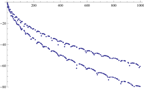
Figure 1. The ($\log$ of the) contributions of the $p^{\text{th}}$ coefficients, for $p<1000$, for two example equations in the case of functional equation (2.2) with $N=211$.

Proving precise estimates that are useful for small $n$ can be difficult: see [12] for details.

6. Solving the system

We continue with (5.15), which must be satisfied by any L-function with conductor $N=211$ and sign $\varepsilon=1$.

Since $2\nmid 211$, there are 35 possible local factors at $p=2$ in the Euler product, as indicated in Table 1. Here are two of them:

$$L_{2,9}(z)=\mathstrut \left(1+\frac{1}{\sqrt{2}}\,z+\frac{1}{\sqrt{2}}\,z^{3}+z^{4}\right)^{-1}$$ (6.1)

$$=\mathstrut 1-\frac{1}{\sqrt{2}}\,z+\frac{1}{{2}}\,z^{2}-\frac{3}{\sqrt{2}}\,z^{3}+\frac{1}{{4}}\,z^{4}+\frac{1}{4\sqrt{2}}\,z^{5}+\cdots$$ (6.2)

$$L_{2,29}(z)=\mathstrut \left(1-{\sqrt{2}}\,z+z^{2}-{\sqrt{2}}\,z^{3}+z^{4}\right)^{-1}$$ (6.3)

$$=\mathstrut 1+{\sqrt{2}}\,z+\,z^{2}+{\sqrt{2}}\,z^{3}+{{2}}\,z^{4}+{\sqrt{2}}\,z^{5}+\cdots.$$ (6.4)

The indices 9 and 29 indicate where those polynomials fall among the list of 35 possible local factors, when ordered lexicographically. Note that $b_{2^{m}}$ is the coefficient of $z^{m}$.

When we substitute the two examples above into (5.15), use the multiplicative relations among the coefficients, and gather terms, we find

$$L_{2,9}:\phantom{xxxxx}0=\mathstrut 1.106\underline{0}+0.375\underline{0}\,b_{3}+0.096\underline{5}\,b_{5}+0.025\underline{4}\,b_{7}+0.0068\underline{2}\,b_{9}$$ (6.5)

$$+0.0018\underline{1}\,b_{11}+0.00046\underline{0}\,b_{13}+0.00010\underline{5}\,b_{15}+0.000020\underline{0}\,b_{17}$$ (6.6)

$$\cdots$$ (6.7)

$$+1.2\underline{5}\times 10^{-8}\,b_{49}+5.4\underline{7}\times 10^{-9}\,b_{51}+1.8\underline{1}\times 10^{-9}\,b_{53}$$ (6.8)

$$\cdots$$ (6.9)

$$L_{2,29}:\phantom{xxxxx}0=\mathstrut 3.045\underline{5}+0.481\underline{5}\,b_{3}+0.104\underline{0}\,b_{5}+0.025\underline{8}\,b_{7}+0.0068\underline{4}\,b_{9}$$ (6.10)

$$+0.0018\underline{2}\,b_{11}+0.00046\underline{6}\,b_{13}+0.00010\underline{8}\,b_{15}+0.000021\underline{7}\,b_{17}$$ (6.11)

$$\cdots$$ (6.12)

$$+1.2\underline{5}\times 10^{-8}\,b_{49}+5.4\underline{7}\times 10^{-9}\,b_{51}+1.8\underline{1}\times 10^{-9}\,b_{53}$$ (6.13)

$$\cdots.$$

If we now use the bounds $|b_{p}|\leq 4$ and $|b_{p^{2}}|\leq 10$, and write “$\pm X$” to indicate a real number in the interval $[-X,X]$, we find

$$L_{2,9}:\phantom{xxxxx}0=\mathstrut 1.106\underline{0}\pm 2.067$$ (6.14)

$$L_{2,29}:\phantom{xxxxx}0=\mathstrut 3.045\underline{5}\pm 2.525\,.$$ (6.15)

The first equation is true, and the second equation is false. Thus, the local factor $L_{2,29}$ cannot occur in any L-function satisfying our assumptions. By creating several equations along the lines described above, one can prove that 15 out of the 35 possible local factors at $p=2$ cannot occur in an L-function satisfying our assumptions.

What can we do about the 20 local factors at $p=2$ that appear to be possible? We move on to the possible local factors at $p=3$. That is, for each of the 20 remaining factors at $p=2$, we consider each of the 63 possible factors at $p=3$. To give one more numerical example, if we use the $25^{th}$ choice for the local factor at $p=3$ in (6.9) we find:

$$L_{2,9}\text{ and }L_{3,25}:\phantom{xxxxx}0=\mathstrut 0.87817\underline{6}+0.096\underline{4}\,b_{5}+0.025\underline{4}\,b_{7}+0.0018\underline{1}\,b_{11}$$ (6.16)

$$+0.0004\underline{6}\,b_{13}+0.0000\underline{2}\,b_{17}+3.7\underline{4}\times 10^{-6}\,b_{19}$$ (6.17)

$$\cdots.$$ (6.18)

Since $|b_{p}|\leq 4$, we see that the above equation cannot be satisfied by the coefficients of any L-function. This rules out the combination $L_{2,9}L_{3,25}$ in the Euler product.

As we proceed in this manner, one of two things can happen. We may find that every choice of coefficients for a given $p$ leads to an equation which cannot be satisfied. That proves there does not exist an L-function with the given functional equation, and therefore there does not exist any object which would have an L-function with such a functional equation.

Or, we could find that, after searching through the first 100 coefficients, there are combinations which are consistent with the equations we form. This proves that only those combinations of coefficients are possible for any L-function with the given functional equation. However, it does not prove that such an L-function exists.

We now give more details about how we organize the search through the coefficients.

7. Searching the tree

The procedure described in Section 6 involves a breadth-first search of a tree, where we prune nodes which have been found to be inconsistent with a possible solution to the system of equations.

We use the entire local factor at the primes $p=2$ and $3$. For larger $p$, we search through the possible $b_{p}$ and $b_{p^{2}}$ separately. This is helpful because, for example, when considering $b_{5}$, the value of $b_{25}$ proportionally contributes very little to the sum: see the plots in Figure 1. Thus, we need only consider the 17 possible values of $b_{5}$, instead of the 129 possible values of $F_{5}$.

Since the running time of the tree search is proportional to the number of equations used when testing candidate coefficients, it is desirable to use few equations. That is, having a small number of equations is preferred provided that the equations are useful for testing the candidate coefficients.

The logical extreme, which was previously employed in [8], is to construct a single equation which has been optimized to minimize the contributions of those coefficients that contribute to the error term. This is easily accomplished (using least squares, for example) by taking a linear combination of the available equations. Figure 2 illustrates an example where we have chosen to minimize the contributions of the coefficients $b_{p}$ for $p\geq 23$. As we are testing possible values of $b_{19}$ using that equation, the error term from the larger coefficients will be small. So one should expect that at most one of those possible choices of $b_{19}$ will lead to a consistent equation. See [8] for more discussion on this approach.

To illustrate the effectiveness of the method, the following is a summary of two sample runs. Each list contains the number of viable possibilities at each depth of searching the tree. For example, in the case of $N=209$ and $\varepsilon=1$, when considering only $p=2$, there were 20 possible values (out of 35) that led to a consistent equation. Then after testing every possible value with $p=3$ for each of those 20 possibilities, a total of 87 combinations remained. Then there were 44 possible combinations for $p=2$, 3, and 5 that survived, and so on.

$$N=209,\ \varepsilon=1:\ \ \ \ \ \ \ \ \ \ \ \ \ \ \{20,87,44,4,1,1,1,1,1,1,1,1,1,2,1,1,1,1,1,1,1,1\}$$ (7.1)

$$N=211,\ \varepsilon=1:\ \ \ \ \ \ \ \ \ \ \ \ \ \ \{20,91,39,1,1,0\}$$ (7.2)

From (7.1) it appears that there is an L-function with $N=209$ and $\varepsilon=1$. Indeed, $L(s,E_{11})L(s,E_{19})$ is such an L-function. From (7.1) it appears that there is exactly one L-function, but as mentioned in Section 2.6, the most we can say is that there is a unique choice of the first 100 coefficients. Current methods do not make it possible to prove there are not several L-functions  which all begin with those same 100 coefficients.

From (7.2) we see that after considering all possible values of $b_{11}$, we have proven that there is no L-function with $N=211$ and $\varepsilon=1$.

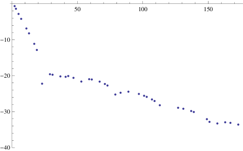
Figure 2. The ($\log$ of the) contributions of the $p^{\text{th}}$ coefficients for one equation made from a linear combination of 11 of our basic equations.

8. Conductor 550

Poor and Yuen [14] have identified a paramodular form of level 550, which by the Paramodular Conjecture [4] is associated to an Abelian surface of conductor 550. Such an Abelian surface has yet to be identified, so to assist in its search, we provide some data about the L-function  of conductor 550 which arose in our search.

Table 2 provides the first few local factors or Dirichlet coefficients, using the notation in Section 2.1. The local factor at $p=3$ agrees with that found by Poor and Yuen.

$p$	$G_{p}(T)$		$p$	$A_{p}$
2	$(1+T)(1+2T^{2})$		17	$-3$
3	$1-T^{2}+9T^{4}$		19	$1$
5	$1+3T+5T^{2}$		23	$-3$
7	$1+4T^{2}+49T^{4}$		29	$0$
11	$(1+T)(1-3T+11T^{2})$		31	$-5$
13	$1-8T^{2}+169T^{4}$		37	$3$

Table 2. Local factors and Dirichlet coefficients of the primitive L-function of degree 4, weight 1, and conductor $N=550$

References

- [1] A. Booker, Numerical tests of modularity. J. Ramanujan Math. Soc. 20 (2005), no. 4, 283–339.
- [2] A. Booker, J. Sijsling, A. Sutherland, John Voight, and Dan Yasaki, A database of genus 2 curves over the rational numbers, Algorithmic Number Theory 12th International Symposium (ANTS XII), LMS Journal of Computation and Mathematics 19 (2016), 235-254.
- [3] C. Bian, Computing GL(3) automorphic forms. Bull. Lond. Math. Soc. 42 (2010), no. 5, 827–842.
- [4] A. Brumer and K. Kramer, Paramodular abelian varieties of odd conductor. Trans. Amer. Math. Soc. 366 (2014), no. 5, 2463-2516.
- [5] J. E. Cremona, Hyperbolic tessellations, modular symbols, and elliptic curves over complex quadratic fields. Compositio Math. 51 (1984), no. 3, 275-324.
- [6] D. Farmer, S. Koutsoliotas, and S. Lemurell, Maass forms on GL(3) and GL(4), Int Math Res Notices 2014 (22): 6276-6301. doi: 10.1093/imrn/rnt145 arXiv:1212.4545
- [7] D. Farmer, A. Pitale, N. Ryan, and R. Schmidt, Analytic L-functions: Definitions, Theorems, and Connections, preprint, arXiv:1711.10375.
- [8] D. Farmer and N. Ryan, Evaluating L-functions with few known coefficients, LMS J. Comput. Math. 17 (2014), no. 1, 245-258. arXiv:1211.4181
- [9] The LMFDB Collaboration, The L-functions and Modular Forms Database, http://www.LMFDB.org [Online: accessed November 20, 2014].
- [10] N. Freitas, B. Le Hung, and S. Siksek Elliptic Curves over Real Quadratic Fields are Modular arXiv:1310.7088
- [11] J.-F. Mestre, Formules explicites et minorations de conducteurs de variétés algébriques. Compositio Math. 58 (1986), no. 2, 209-232.
- [12] P. Molin, Intégration numérique et calculs de fonctions L, PhD Thesis, Institut de Mathématiques de Bordeaux, 2010.
- [13] C. Poor and D. S. Yuen, Paramodular Cusp Forms, arXiv:0912.0049
- [14] C. Poor and D. S. Yuen, personal communication.
- [15] M. Rubinstein, Computational methods and experiments in analytic number theory, in, “Recent perspectives in random matrix theory and number theory”, F.Mezzadri and N.C.Snaith, Eds, LMS 2005.
- [16] Schoof, René Abelian varieties over Q with bad reduction in one prime only. Compos. Math. 141 (2005), no. 4, 847-868.
- [17] A. Selberg, Old and new results and conjectures about a class of Dirichlet series, Proceedings of the Amalfi Conference on Analytic Number Theory 1989, Univ. Salerno, Salerno (1992), 367–385.
- [18] http://www.mathe2.uni-bayreuth.de/stoll/