Abstract

This note aims at demonstrating the advantage of moving-water well-balanced schemes over still-water well-balanced schemes for the shallow water equations. We concentrate on numerical examples with solutions near a moving-water equilibrium. For such examples, still-water well-balanced methods are not capable of capturing the small perturbations of the moving-water equilibrium and may generate significant spurious oscillations, unless an extremely refined mesh is used. On the other hand, moving-water well-balanced methods perform well in these tests. The numerical examples in this note clearly demonstrate the importance of utilizing moving-water well-balanced methods for solutions near a moving-water equilibrium.

Keywords: shallow water equation, still water, moving water equilibrium, high order accuracy, well-balanced scheme

1 Introduction

The main objective of this note is to demonstrate the advantage of schemes which are well balanced for moving water equilibrium, over those which are only well balanced for still water, for small perturbations of the moving water equilibrium for the shallow water equations.

Well-balanced schemes refer to those schemes which have zero truncation error for certain steady-state solutions of hyperbolic balance laws

$$U_{t}+f(U)_{x}=g(U,x).$$

That is, for certain non-trivial functions $V(x)$ satisfying

$$f(V)_{x}=g(V,x),$$

the well balanced schemes do not have any truncation error. Note that in general $V(x)$ is unknown and is not a polynomial, thus to require a zero truncation error is a difficult task.

For shallow water equations, there are typically two classes of well-balanced schemes, namely those which are well balanced for still-water equilibrium, where the velocity is zero, and those which are well balanced for general moving-water equilibrium. A scheme which belongs to the latter class is more difficult to construct. We refer to [1] for a recently developed high-order accurate finite volume weighted essentially non-oscillatory (WENO) scheme which is well balanced for general moving-water equilibrium. Discussions on the history of the development of well balanced schemes for shallow water equations, with an extensive reference list, can be found in [2].

Since it is much more difficult to construct well-balanced schemes for moving-water equilibrium than for still water, a natural question is whether the former has any advantage over the latter. However, to our best knowledge, examples to show this advantage seem to be absent in the literature. In the Castro Urdiales meeting for which this special issue is dedicated to, there was an intense discussion on this issue but no such examples were provided in the discussion.

The purpose of this note is therefore to provide carefully selected numerical examples to demonstrate the advantage of well-balanced schemes for moving-water equilibrium over well-balanced schemes for still water. These examples have solutions which contain small perturbations from a moving-water equilibrium. A well-balanced scheme for still water would generate spurious oscillations at the level of the truncation error of the scheme, until the mesh is extremely refined. On the other hand, a well-balanced scheme for the moving-water equilibrium could resolve these small perturbations on much coarser meshes. These examples clearly demonstrate the advantage of well-balanced schemes for moving-water equilibrium. We shall use the high order finite volume WENO schemes in [4], which are well balanced for still water, and those in [1], which are well balanced for moving water, in the numerical tests.

2 Shallow water equations and well-balanced methods

In one space dimension, the shallow water equations take the form

$$\left\{\begin{array}[]{l}\displaystyle h_{t}+(hu)_{x}=0\\ \displaystyle(hu)_{t}+\left(hu^{2}+\frac{1}{2}gh^{2}\right)_{x}=-ghb_{x},\end{array}\right.$$ (2.1)

where $h$ denotes the water height, $u$ is the velocity of the fluid, $b$ represents the bottom topography and $g$ is the gravitational constant. The still-water (also referred as lake at rest) steady state is given by

$$u=0\qquad\text{and}\qquad h+b=const,$$ (2.2)

which represents a still flat water surface. The general moving-water steady state is given by

$$m=hu=const\qquad\text{and}\qquad E=\frac{1}{2}u^{2}+g(h+b)=const.$$ (2.3)

We introduce the notation $U=(h,\,hu)^{T}$ for the conservative variables, with the superscript $T$ denoting the transpose, and $V=(m,\,E)^{T}$ for the equilibrium variables. We refer to [1] for the variable transformation between $U=U(V,x)$ and $V=V(U,x)$.

The computational domain is discretized into cells $I_{i}=[x_{i-\frac{1}{2}},x_{i+\frac{1}{2}}]$, $i=1,\cdots,N$. We denote the size of the $i$-th cell by $\triangle x_{i}$ and the center of the cell by $x_{i}=\left(x_{i-\frac{1}{2}}+x_{i+\frac{1}{2}}\right)/2$. Let $\bar{U}(x_{i},t)=\int_{I_{i}}U(x,t)\,dx/\triangle x_{i}$ denote the cell average of $U(\cdot,t)$ over the cell $I_{i}$. The computational variables are $\bar{U}^{n}_{i}$, which approximate the cell averages $\bar{U}(x_{i},t)$ at the time $t=t^{n}$. For the ease of presentation, we denote the shallow water equations (2.1) by

$$U_{t}+f(U)_{x}=g(h,b).$$

2.1 Methods preserving still-water equilibrium

Many high-order well-balanced methods for the still-water steady state solution (2.2) have been developed in the literature for the shallow water equations, see for example [2] for a list of references. In this note, we will use the fifth-order finite volume WENO methods based on the separation of the source terms developed in Xing and Shu [4]. In this subsection, we briefly review this well-balanced scheme in one dimension. We refer to [4] for further details.

We first reconstruct the point values $U^{\pm}_{i+\frac{1}{2}}$ at the cell interface from the given cell averages $\bar{U}_{i}$ by the standard WENO reconstruction procedure, which can be eventually written out as

$$U_{i+\frac{1}{2}}^{+}=\sum_{k=-r+1}^{r}w_{k}\bar{U}_{i+k}\equiv S^{+}_{\bar{U}}(\bar{U})_{i},\qquad U_{i+\frac{1}{2}}^{-}=\sum_{k=-r}^{r-1}\tilde{w}_{k}\bar{U}_{i+k}\equiv S^{-}_{\bar{U}}(\bar{U})_{i}$$ (2.4)

where $r=3$ for the fifth order WENO approximation and the coefficients $w_{k}$ and $\tilde{w}_{k}$ depend nonlinearly on $\bar{U}$. Now we freeze the cell averages $\bar{U}$ and the corresponding coefficients $w_{k}$ and $\tilde{w}_{k}$. With these fixed coefficients, we apply the linear operators $W\mapsto S^{\pm}_{\bar{U}}(W)$ to $W=(b,0)^{T}$ to compute the reconstructed values $b^{\pm}_{i+\frac{1}{2}}$. Assume $U$ is the still-water steady state solution satisfying (2.2), we clearly have

$$h^{\pm}_{i+\frac{1}{2}}+b^{\pm}_{i+\frac{1}{2}}=constant.$$ (2.5)

The main idea in constructing well-balanced methods is to decompose the integral of the source term into a sum of several terms, then compute each of them in a way consistent with the approximation for the corresponding flux terms. We first rewrite the shallow water equations (2.1) as

$$\left\{\begin{array}[]{l}\displaystyle h_{t}+(hu)_{x}=0\\ \displaystyle(hu)_{t}+\left(hu^{2}+\frac{1}{2}gh^{2}\right)_{x}=\left(\frac{1}{2}gb^{2}\right)_{x}-g(h+b)b_{x},\end{array}\right.$$ (2.6)

for which the semi-discrete numerical method takes the form

$$\triangle x_{i}\frac{d\bar{U}(x_{i},t)}{dt}=-(\hat{F}_{i+\frac{1}{2}}-\hat{F}_{i-\frac{1}{2}})+G(U,x),$$ (2.7)

where $\hat{F}$ is a numerical flux, such as the Lax-Friedrichs flux

$$\hat{F}_{i+\frac{1}{2}}=\frac{1}{2}\left[f(U^{-}_{i+\frac{1}{2}})+f(U^{+}_{i+\frac{1}{2}})-\alpha\left(\left(\begin{array}[]{c}h+b\\ hu\end{array}\right)^{+}_{i+\frac{1}{2}}-\left(\begin{array}[]{c}h+b\\ hu\end{array}\right)^{-}_{i+\frac{1}{2}}\right)\right],$$ (2.8)

with $\alpha=\max_{U}|u\pm\sqrt{gh}|$. The first component of the source term approximation $G(U,x)$ is zero, and the second component is given by

$$\frac{1}{2}g\left(\widehat{b_{i+\frac{1}{2}}^{2}}-\widehat{b_{i-\frac{1}{2}}^{2}}\right)-g\overline{(h+b)}_{i}(\hat{b}_{i+\frac{1}{2}}-\hat{b}_{i-\frac{1}{2}})-\int_{I_{i}}g\left(h+b-\overline{(h+b)}_{i}\right)b_{x}dx,$$ (2.9)

with $\widehat{b^{2}_{i+\frac{1}{2}}}=\frac{1}{2}\left((b^{+}_{i+\frac{1}{2}})^{2}+(b^{-}_{i+\frac{1}{2}})^{2}\right)$ and $\hat{b}_{i+\frac{1}{2}}=\frac{1}{2}(b^{+}_{i+\frac{1}{2}}+b^{-}_{i+\frac{1}{2}})$.

2.2 Methods preserving moving-water equilibrium

We have developed high-order well-balanced finite volume WENO schemes for the moving-water equilibrium (2.3) for the shallow water equations in [1]. In this subsection, we briefly review these methods and refer to [1] for further details.

At each time step, we first apply the usual WENO reconstruction procedure to the cell averages $\bar{U}_{i}$, and obtain $U^{\pm}_{i+\frac{1}{2}}$, hence $V^{\pm}_{i+\frac{1}{2}}$.

Given the cell averages $\bar{U_{i}}$ and a bottom function $b(x)$, we choose local reference values $\bar{V_{i}}$ of the equilibrium variables. These are defined implicitly by the requirement that

$$\frac{1}{\Delta x_{i}}\int_{I_{i}}U(\bar{V}_{i},x)dx=\bar{U}_{i}.$$ (2.10)

Relation (2.10) chooses $\bar{V}_{i}$ as the unique (see the paragraphs preceding [1, Def.3.2]) local equilibrium such that the corresponding conserved variables $U(\bar{V}_{i},b(x))$ have the same cell average $\bar{U}_{i}$ as the numerical data. It is proven in [1, Def.3.2] that, if the data $U(x)$ and $b(x)$ are in local equilibrium ($V(U(x),x)\equiv\bar{V}$ for all cells $I_{i}$), the reference equilibrium states $\bar{V}_{i}$ computed via (2.10) coincide with the true local steady state $\bar{V}$. The reconstruction is completed by limiting the reconstruction $V^{\pm}_{i+\frac{1}{2}}$ with respect to the reference values $\bar{V}_{i}$ (see [1, (3.18)]), to obtain the limited values $\tilde{V}^{\pm}_{i+\frac{1}{2}}$ and $\tilde{V}_{i}$.

The fourth-order well-balanced scheme is given by

$$\triangle x_{i}\frac{d\bar{U}(x_{i},t)}{dt}=-(\hat{F}(\hat{U}_{i+\frac{1}{2}}^{-},\hat{U}_{i+\frac{1}{2}}^{+})-\hat{F}(\hat{U}_{i-\frac{1}{2}}^{-},\hat{U}_{i-\frac{1}{2}}^{+}))+s_{i},$$ (2.11)

where the function $\hat{F}(\cdot,\cdot)$ is a conservative, Lipschitz continuous numerical flux, and

$$\hat{U}_{i+\frac{1}{2}}^{\pm}=U(\tilde{V}_{i+\frac{1}{2}}^{\pm},\hat{b}_{i+\frac{1}{2}}),\qquad\hat{b}_{i+\frac{1}{2}}=\min(b_{i+\frac{1}{2}}^{-},b_{i+\frac{1}{2}}^{+}).$$ (2.12)

The total source term $s_{i}$ is given by

$$s_{i}:=\frac{\displaystyle 4S_{2}-S_{1}}{3}+f(\hat{U}_{i-\frac{1}{2}}^{+})-f(\tilde{U}_{i-\frac{1}{2}}^{+})+f(\tilde{U}_{i+\frac{1}{2}}^{-})-f(\hat{U}_{i+\frac{1}{2}}^{-}),$$ (2.13)

where $\tilde{U}_{i-\frac{1}{2}}^{\pm}=U(\tilde{V}_{i+\frac{1}{2}}^{\pm},b_{i+\frac{1}{2}}^{\pm})$. The extrapolated interior source term $(4S_{2}-S_{1})/3$ is defined by

$$S_{1} = s_{i}^{int}(\tilde{U}^{+}_{i-\frac{1}{2}},\tilde{U}^{-}_{i+\frac{1}{2}},b^{+}_{i-\frac{1}{2}},b^{-}_{i+\frac{1}{2}})$$ (2.14)

$$S_{2} = \left(s_{i}^{int}(\tilde{U}^{+}_{i-\frac{1}{2}},\tilde{U}_{i},b^{+}_{i-\frac{1}{2}},b_{i})+s_{i}^{int}(\tilde{U}_{i},\tilde{U}^{-}_{i+\frac{1}{2}},b_{i},b^{-}_{i+\frac{1}{2}})\right)$$ (2.15)

and the well-balanced quadrature of the source term $s_{i}^{int}$ is given by

$$s_{i}^{int}(U_{L},U_{R},b_{L},b_{R})=-\frac{1}{2}g(h_{L}+h_{R})(b_{R}-b_{L})+\hat{s}_{i}^{int}$$ (2.16)

where $\hat{s}_{i}^{int}$ is given by [1, (3.63)-(3.65)].

3 Numerical examples

In this section we present numerical results of both moving-water well-balanced methods and still-water well-balanced methods presented in Section 2, for a carefully selected set of test examples in one dimension. Comparison of these results is provided as a demonstration of the advantage of moving-water well-balanced methods. In all the examples, time discretization is by the classical third-order total variation diminishing (TVD) Runge-Kutta method [3], and the CFL number is taken as 0.6. The gravitation constant $g$ is taken as 9.812$m/s^{2}$.

3.1 Perturbation of a moving water equilibrium

The following test cases are chosen to demonstrate the capability of these schemes for computations on the perturbation of steady state solutions.

The bottom topography is given by:

$$b(x)=\left\{\begin{array}[]{l l}0.2-0.05(x-10)^{2}&\mbox{if }8\leq x\leq 12,\\ 0&\mbox{otherwise,}\end{array}\right.$$ (3.1)

in the computational domain $[0,25]$. Three steady states, subcritical or transcritical flow with or without a steady shock will be investigated.

Our initial conditions are given by imposing a small perturbation of size $0.05$ on the height of these steady states in the interval $[5.75,\,6.25]$. Theoretically, this disturbance should split into two waves, propagating to the left and right respectively. Note that in [1], we have shown the numerical results of the moving-water well-balanced methods with a perturbation size $0.01$, which demonstrate that these small perturbations are well captured. Here we provide the numerical results of both the moving-water well-balanced methods and still-water well-balanced methods, and demonstrate the different behavior of these two methods.

a): Subcritical flow:

The initial condition is given by:

$$E=22.06605,\qquad m=4.42,$$ (3.2)

together with the boundary condition that the discharge $m$=4.42 is imposed at upstream and the water height $h$=2 is imposed at downstream when the flow is subcritical.

We run the tests with 100 uniform cells until $t=1.5$, when the downstream-traveling water pulse has already passed the bump. The differences between the water height $h$ at that time and the background moving water state, are shown in Figure 3.1. The result of the still-water well-balanced method is plotted on the left and that of the moving-water well-balanced method is shown on the right. The difference can be easily observed, as there are significantly more spurious oscillations generated by the still-water well-balanced method. As we refine the mesh to $1000$ cells, the results are shown in Figure 3.2. Because $\Delta x$ is now very small, the perturbation is relatively big in comparison with truncation errors of the schemes and can be well captured by both methods.

 

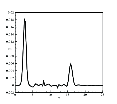
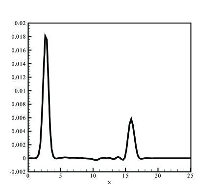
Figure 3.1: The difference between the height $h$ at time $t=1.5$ and the background moving steady state water height (3.2), when 100 uniform cells are employed. An initial perturbation of size $0.05$ is imposed between $[5.75,\,6.25]$. Left: result based on still-water well-balanced scheme. Right: result based on moving-water well-balanced scheme.

 

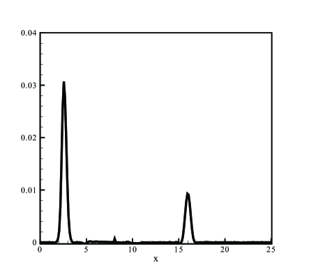
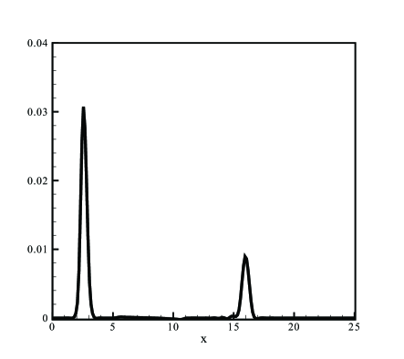
Figure 3.2: Same as in Figure 3.1, but 1000 uniform cells are employed.

b): Transcritical flow without a shock:

The initial condition is given by:

$$E=\frac{1.53^{2}}{2\times 0.66^{2}}+9.812\times 0.66,\qquad m=1.53,$$ (3.3)

together with the boundary condition that the discharge $m$=1.53 is imposed at upstream and the water height $h$=0.66 is imposed at downstream when the flow is subcritical.

We run the tests with 100 uniform cells until $t=1.5$, when the downstream-traveling water pulse has already passed the bump. The differences between the water height $h$ at that time and the background moving water state, are shown in Figure 3.3. Again, the difference can be easily observed, as there are significantly more spurious oscillations generated by the still-water well-balanced method. As we refine the mesh to $1000$ cells, the results in Figure 3.4 show resolved solutions for both methods.

 

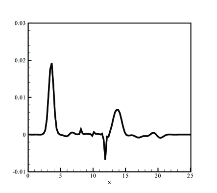
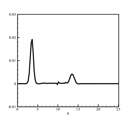
Figure 3.3: The difference between the height $h$ at time $t=1.5$ and the background moving steady state water height (3.3), when 100 uniform cells are employed. An initial perturbation of size $0.05$ is imposed between $[5.75,\,6.25]$. Left: result based on still-water well-balanced scheme. Right: result based on moving-water well-balanced scheme.

 

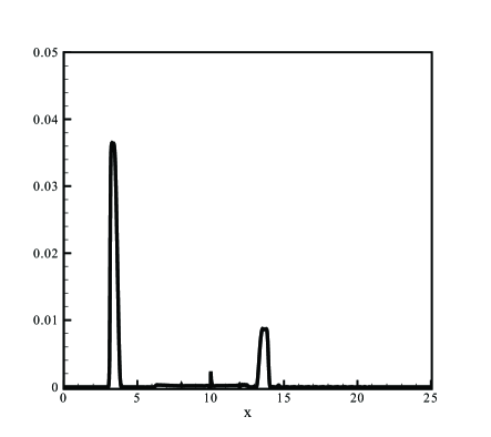
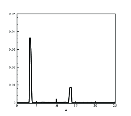
Figure 3.4: Same as in Figure 3.3, but 1000 uniform cells are employed.

c): Transcritical flow with a shock:

The initial condition is given by:

$$E=\left\{\begin{array}[]{l l}\frac{3}{2}(9.812\times 0.18)^{\frac{2}{3}})+9.812\times 0.2\par&\mbox{if }x\leq 11.665504281554291\\ \frac{\displaystyle 0.18^{2}}{\displaystyle 2\times 0.33^{2}}+9.812\times 0.33&\mbox{otherwise}\end{array}\right.\qquad m=0.18,$$ (3.4)

together with the boundary condition that the discharge $m$=0.18 is imposed at upstream and the water height $h$=0.33 is imposed at downstream.

We run the tests with 200 uniform cells until $t=3$. The differences between the water height $h$ at that time and the background moving water state, are shown in Figure 3.5. Once again, the difference can be easily observed, as there are significantly more spurious structures generated by the still-water well-balanced method. As we refine the mesh to $1000$ cells, the results are shown in Figure 3.6. Even at this resolution there is still an advantage using the moving-water well-balanced method. Note that near the point $x=11.7$ there is a big displacement for both methods, as we recall that $11.7$ is the position where the shock is located.

 

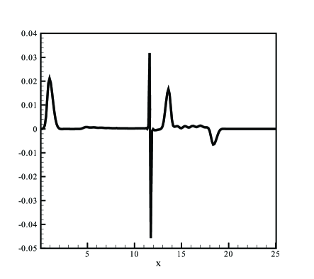
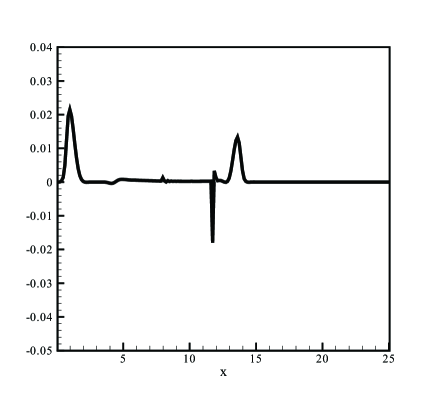
Figure 3.5: The difference between the height $h$ at time $t=3$ and the background moving steady state water height (3.4), when 200 uniform cells are employed. An initial perturbation of size $0.05$ is imposed between $[5.75,\,6.25]$. Left: result based on still-water well-balanced scheme. Right: result based on moving-water well-balanced scheme.

 

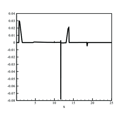
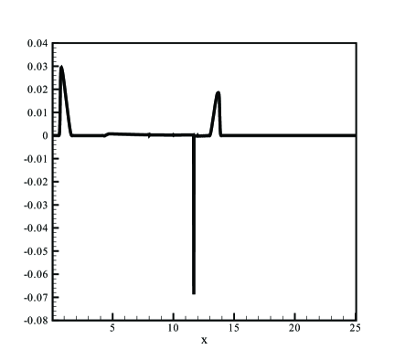
Figure 3.6: Same as in Figure 3.5, but 1000 uniform cells are employed.

3.2 Perturbation with smaller magnitude

In this subsection, we utilize a smaller perturbation to these tests and show that moving-water well-balanced methods demonstrate more clearly their advantage in capturing such perturbations.

We keep the main setup the same as in Section 3.1, and impose a smaller perturbation of size $0.001$ to these steady states. To save space, only the results of the subcritical flow (3.2) are shown. The differences between the water height $h$ at that time and the background moving water state, when 100 uniform cells are used, are plotted in Figure 3.7. We also show the differences of the momentum $hu$ in Figure 3.8. These figures clearly demonstrate that the still-water well-balanced method is not capable of capturing such a small perturbation on the coarse mesh, as large spurious oscillations are observed. As we refine the meshes to 200 cells, the results are shown in Figures 3.9 and 3.10, where spurious oscillations for the still-water well-balanced method have a reduced magnitude, but its performance is still significantly inferior to that of the moving-water well-balanced method. The results with $1000$ cells are shown in Figures 3.11 and 3.12. Even though the difference between the two methods is now significantly reduced, the advantage of the moving-water well-balanced method can still be observed on such a refined mesh.

 

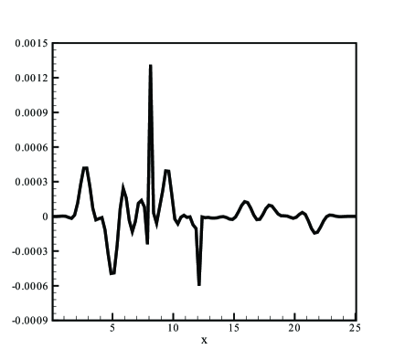
Figure 3.7: The difference between the height $h$ at time $t=1.5$ and the background moving steady state water height (3.2), when 100 uniform cells are employed. An initial perturbation of size $0.001$ is imposed between $[5.75,\,6.25]$. Left: result based on still-water well-balanced scheme. Right: result based on moving-water well-balanced scheme.

 

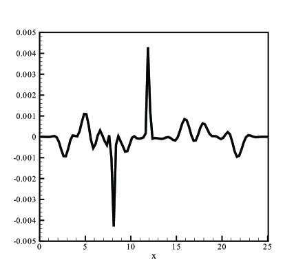
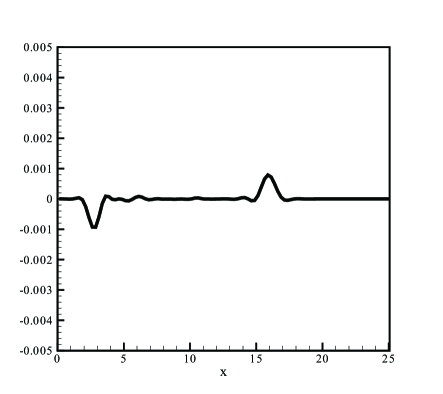
Figure 3.8: The difference between the momentum $hv$ at time $t=1.5$ and the background moving steady state water height (3.2), when 100 uniform cells are employed. An initial perturbation of size $0.001$ is imposed between $[5.75,\,6.25]$. Left: result based on still-water well-balanced scheme. Right: result based on moving-water well-balanced scheme.

 

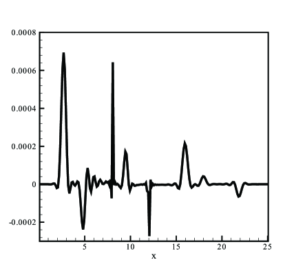
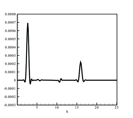
Figure 3.9: Same as in Figure 3.7, but 200 uniform cells are employed.

 

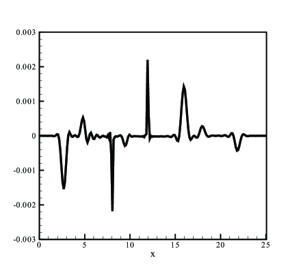
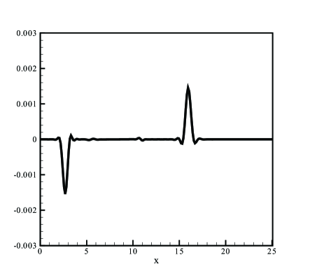
Figure 3.10: Same as in Figure 3.8, but 200 uniform cells are employed.

 

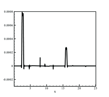
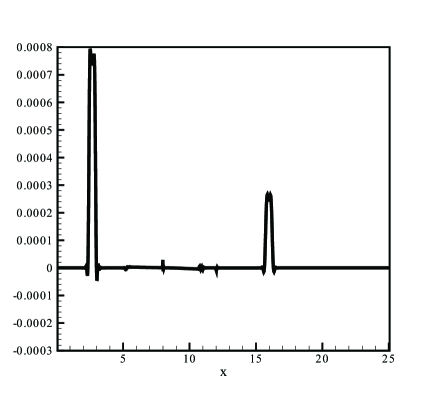
Figure 3.11: Same as in Figure 3.7, but 1000 uniform cells are employed.

 

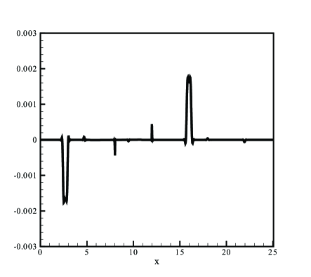
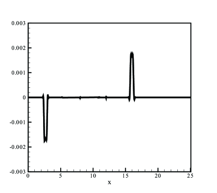
Figure 3.12: Same as in Figure 3.8, but 1000 uniform cells are employed.

Acknowledgement. The first author is a contractor [UT-Battelle, manager of Oak Ridge National Laboratory] of the U.S. Government under Contract No. DE-AC05-00OR22725. Accordingly, the U.S. Government retains a non-exclusive, royalty-free license to publish or reproduce the published form of this contribution, or allow others to do so, for U.S. Government purposes.

References

- [1] S. Noelle, Y. Xing and C.-W. Shu, High order well-balanced finite volume WENO schemes for shallow water equation with moving water, J. Comput. Phys. 226 (2007), 29-58.
- [2] S. Noelle, Y. Xing and C.-W. Shu, High order well-balanced schemes, to appear in Numerical Methods for Relaxation Systems and Balance Equations, G. Puppo and G. Russo, editors, Quaderni di Matematica, Dipartimento di Matematica, Seconda Universita di Napoli, Italy.
- [3] C.-W. Shu and S. Osher, Efficient implementation of essentially non-oscillatory shock-capturing schemes, J. Comput. Phys. 77 (1988), 439-471.
- [4] Y. Xing and C.-W. Shu, High order well-balanced finite volume WENO schemes and discontinuous Galerkin methods for a class of hyperbolic systems with source terms, J. Comput. Phys. 214 (2006), 567-598.