An early warning indicator for atmospheric blocking events using transfer operators

Abstract

The existence of persistent midlatitude atmospheric flow regimes with time-scales larger than 5-10 days and indications of preferred transitions between them motivates to develop early warning indicators for such regime transitions. In this paper, we use a hemispheric barotropic model together with estimates of transfer operators on a reduced phase space to develop an early warning indicator of the zonal to blocked flow transition in this model. It is shown that, the spectrum of the transfer operators can be used to study the slow dynamics of the flow as well as the non-Markovian character of the reduction. The slowest motions are thereby found to have time scales of three to six weeks and to be associated with meta-stable regimes (and their transitions) which can be detected as almost-invariant sets of the transfer operator. From the energy budget of the model, we are able to explain the meta-stability of the regimes and the existence of preferred transition paths. Even though the model is highly simplified, the skill of the early warning indicator is promising, suggesting that the transfer operator approach can be used in parallel to an operational deterministic model for stochastic prediction or to assess forecast uncertainty.

The transfer operator of a model of the atmosphere is used to isolate and detect persistent atmospheric regimes and to define an early warning indicator of transitions between these regimes. The methodology is expected to have application potential to general dissipative chaotic systems.

I introduction

The midlatitude atmospheric flow is considered to be a chaotic dynamical system for which predictability is limited (Lorenz, 1963; Palmer, 1993). Although the behavior of this flow is dominated by weather systems on short time scales caused by baroclinic instability, strong variability on time scales longer than 5-10 days, with a predominantly barotropic structure, is also observed (James, 1994). It has been argued that at least part of the observed low-frequency variability can be explained by recurrent and persistent atmospheric regimes (Mo et al., 1988; Kimoto and Ghil, 1993; Smyth et al., 1999) such as the North Atlantic Oscillation (NAO) and blocking events (Plaut and Vautard, 1994; Ghil and Robertson, 2002).

Many studies identifying atmospheric regimes use algorithms relying on the recurrence property of these regimes such as the k-means (Mo et al., 1988; Kondrashov et al., 2004) and the Gaussian mixture algorithms (Smyth et al., 1999; Smyth, 1999). Other studies make use of persistence properties, for example leading to Hidden Markov Models (Majda et al., 2006; Franzke et al., 2008). Most of these techniques rely on the reduction of the high-dimensional phase space to a few dimensions.

The existence of weather regimes in General Circulation Models (GCM) and in reanalysis has been questioned for some time (Stephenson et al., 2004; Christiansen, 2007; Fereday et al., 2008). Using the Integrated Forecast System (IFS) of the European Centre for Medium-Range Weather Forecasts (talk), it was shown (Dawson et al., 2012; Jung et al., 2005; Dawson et al., 2014) that it was necessary to use a spatial resolution of T1279 (16 km), or to include stochastic parametrizations, in order for the atmospheric regime behavior to occur. This suggests that although the atmospheric regimes are large-scale low frequency motions, the faster small-scale motions (either explicitly resolved or included as random perturbations) are important to simulate them.

The barotropic structure of midlatitude low-frequency variability has motivated early studies using low-order barotropic models. Charney and DeVore (1979) have shown that such regimes could manifest themselves in highly truncated spectral barotropic models as stable fixed points representative of different solutions of a standing Rossby wave over topography. Flow regimes and spontaneous transitions have been observed in laboratory experiments using rotating annulus experiments for a barotropic fluid with topography (Weeks et al., 1997) and for a two-layer shear flow (Williams, 2003; Williams et al., 2004, 2005, 2008). In (Weeks et al., 1997), a zonal flow and blocked flow were found for different values of the Rossby number, and spontaneous transitions between the two were observed for intermediate values of the Rossby number. They suggested that these transitions were associated with the existence of two basins of attraction connected by heteroclinic orbits.

A scenario of chaotic itinerancy (Kaneko, 1991; Itoh and Kimoto, 1996) permitted by heteroclinic connections is supported by the study of Crommelin et al. (2004) using a 6-mode barotropic model. For specific values of the forcing parameter, the two stable fixed points of the zonal and blocked regimes merge with a periodic orbit (due to barotropic instability), yielding a heteroclinic connection. Although such a specific situation is unlikely to exist in the real atmosphere, Crommelin (2003) found evidence of ruins of such a heteroclinic connection in a hemispheric barotropic model with realistic topography and forcing (Selten, 1995), manifested by the presence of preferred transition paths. Regime behavior was also found in more realistic barotropic (Legras and Ghil, 1985; Branstator and Opsteegh, 1989; Crommelin, 2003) and multilayer quasi-geostrophic models (Itoh and Kimoto, 1996; Kondrashov et al., 2004). Because these models exhibit chaotic behavior, the regimes are no longer identified by stable fixed points but rather as neighborhoods in the phase space where trajectories tend to persist, motivating their denomination as meta-stable regimes.

In the laboratory experiments by Williams (2003), it is the inertia-gravity waves which are responsible for the regime transitions when the flow is baroclinically unstable. Such waves and barotropic disturbances occur in the real atmosphere together with baroclinically unstable synoptic weather systems, so that it is not yet clear if one disturbance is more important than the other in inducing certain regime transitions. All these possible mechanisms suggest, however, that the variability of the midlatitude atmospheric circulation can be captured by a deterministic model with multiple basins of attraction ‘forced’ by random perturbations representative of high-frequency eddies.

This multi-scale property of the climate system motivates a stochastic-modeling approach (Gardiner, 2009) to climate variability (Penland, 2003). Stochastic climate modeling often relies on a time-scale separation where the state vector is decomposed into a slow climate component and fast weather fluctuations. These fast fluctuations are not resolved explicitly but their aggregated effect is represented by a noise term. The system is thus modeled by a Stochastic Differential Equation (SDE) (Gardiner, 2009) with in general non-linear deterministic terms and additive and/or state-dependent noise terms (Majda et al., 1999, 2001; Franzke et al., 2005, 2015). When the time-scale separation assumption is violated, the Mori-Zwanzig formalism shows that a non-Markovian term representative of the memory effect induced by past interactions between the resolved and the unresolved variables has to be added (Chorin and Hald, 2009; Darve et al., 2009; Wouters and Lucarini, 2013; Kondrashov et al., 2015). Stochastic modeling has been applied to many problems in climate science, such as subgrid-scale parametrization, uncertainty quantification and data assimilation Palmer and Williams (2009); Franzke et al. (2015).

When randomness is present in a dynamical system, whether it is because of uncertainty in the initial state of chaotic systems or because of a stochastic forcing, it is of interest to study the evolution of probability densities in phase space by the flow rather than that of individual trajectories (Lasota and Mackey, 1994; Froyland and Padberg-gehle, 2014). This evolution is given by the transfer operator whose point spectrum, the Ruelle-Policott resonances (Pollicott, 1985; Ruelle, 1986a, b; Butterley and Liverani, 2007; Chekroun et al., 2014), give valuable information on the slow dynamics of the system. For mixing dissipative systems, these resonances are associated with a slow correlation decay and the manifestation of meta-stability (Froyland and Padberg-gehle, 2014).

The main purpose of the present study is to develop an early warning indicator of transitions between atmospheric flow regimes. A traditional method that gives an early warning of a sudden transition is the use of the critical slow down of the system when it gets close to a bifurcation point Scheffer et al. (2009). However, in a high-dimensional model such as that used in (Crommelin, 2003) it is too simplistic to reduce the topology of the system to one or more stable fixed points. Recently, it was shown that complex networks can reveal information on nearby simple bifurcations in high-dimensional dynamical systems (van der Mheen et al., 2013). Near bifurcation points, the topology of the network changes drastically and early warning indicators for transitions were developed based on these topological changes (Viebahn and Dijkstra, 2014; Feng et al., 2014; Tirabassi et al., 2014).

In this study, we base the early warning indicator on the evolution of probability densities with respect to meta-stable regimes in a reduced phase space of the barotropic model used in Crommelin (2003). To study the slow dynamics in this phase space and to evaluate the effect of memory induced by the reduction, the spectrum of transfer operators estimated for different lags is analyzed. Meta-stable regimes are subsequently detected from the transfer operator at a carefully chosen lag. An early warning indicator of transition to the blocked regime is developed from the transfer operator making use of the existence of preferred transition paths between the regimes. To test the quality of the early warning indicator, a traditional method employing the Peirce skill score (Peirce, 1884; Stephenson, 2000; Thornes and Stephenson, 2001) is used. Finally, a study of the energy budget of the barotropic model is performed, where particular attention is given to the conversion of mean kinetic energy to eddy kinetic energy by Reynolds’ stresses, to provide a physical background to the early warning indicator.

II Reduction of the T21-barotropic model

II.1 Model and Data

Transitions between zonal and blocked regimes of the northern hemisphere atmospheric circulation are here investigated using a barotropic model Selten (1995); Crommelin (2003); Franzke et al. (2005). The dimensionless equation of the model, expressed in terms of the streamfunction $\psi$ (representing the non-divergent flow) and using the mean radius of the Earth and the inverse of its rotation rate as horizontal and temporal scale, is given by the barotropic vorticity equation (BVE)

$$\frac{\partial\nabla^{2}\psi}{\partial t}=-\mathcal{J}(\psi,\nabla^{2}\psi+f+h_{b})-k_{1}\nabla^{2}\psi+k_{2}\nabla^{8}\psi+\nabla^{2}\psi^{*},$$ (1)

where $\mathcal{J}$ denotes the Jacobian operator, $f$ the Coriolis parameter, $h_{b}$ the scaled orography, $k_{1}$ the Ekman damping coefficient, $k_{2}$ the coefficient of scale-selective damping and $\nabla^{2}\psi^{*}$ the prescribed vorticity forcing. The non-dimensional orography $h_{b}$ is related to the one of the real Northern Hemisphere $h^{\prime}_{b}$ by

$$h_{b}=2A_{0}\frac{h^{\prime}_{b}}{H}~{}\sin\phi_{0},$$ (2)

where $\phi_{0}=45^{\circ}$N, $A_{0}=0.2$ is a factor determining the strength of the surface winds that blow across the topography, and $H$ is a scale height of 10 km.

The BVE is projected onto spherical harmonics, triangularly truncated at the $21^{st}$ mode (T21). The spherical harmonic coefficients are chosen such that the model is hemispheric with no flow across the equator, resulting in a system of $231$ Ordinary Differential Equations (ODE), which are integrated using a fourth order Runge-Kutta numerical scheme. Following Selten (1995), the Ekman damping time scale and the scale-selective damping time scale were chosen as $15$ days and $3$ days (for wavenumber 21), respectively, so as to adequately reproduce the observed mean and variance of the 500hPa Northern-Hemisphere 10-day mean relative vorticity. The vorticity forcing $\nabla^{2}\psi^{*}$ is calculated from ECMWF reanalysis data of wintertime 500hPa relative vorticity from 1981 to 1991, in order for the first two moments of the simulated relative vorticity to be as close as possible to the observed relative vorticity. The term $\nabla^{2}\psi^{*}$ is calculated (Roads, 1987; Selten, 1995) according to

$$\nabla^{2}\psi^{*}=\mathcal{J}(\psi_{cl},\nabla^{2}\psi_{cl}+f+h_{b})+k_{1}\nabla^{2}\psi_{cl}-k_{2}\nabla^{8}\psi_{cl}+\overline{\mathcal{J}(\psi^{\prime},\nabla^{2}\psi^{\prime})},$$ (3)

where $\psi_{cl}$ is the mean of the observed streamfunction. The quantity $\psi^{\prime}$ is the deviation of the 10-day running mean observed streamfunction from $\psi_{cl}$. The present study relies on a 500,000-day-long simulation using an integration time-step of 30 minutes, with daily output and a spin-up of $5,000$ days removed.

II.2 Phase-space reduction

In order to investigate the presence of meta-stable regimes and preferred transition paths, it is important to define a proper reduction of the $231$-dimensional phase space. This is usually done by projecting the state vector on a low-dimensional basis of orthogonal vectors such that the variance of the projected state vector is maximized. In practice, this can be achieved by an Empirical Orthogonal Function (EOF, e.g von Storch and Zwiers, 1999) analysis of the streamfunction normalized by the kinetic energy norm (Crommelin, 2003; Franzke et al., 2005). The streamfunction patterns of the three leading EOFs are represented in figure 1 and explain $36.7\%$ of the total variance. The first EOF is related to the Arctic Oscillation (AO), blocking events and the strength of the polar vortex (Crommelin, 2003). As it shows a dipole-like pattern over the Atlantic basin, the third EOF has been associated with the North Atlantic Oscillation (NAO).

Figure 1: Dimensionless streamfunction of the three leading EOFs of the barotropic model. EOF 1 (a), EOF 2 (b) and EOF 3 (c) that explain 21.4%, 8.5% and 6.8% of the variance, respectively.

For the purpose of this study, special care must be given to the choice of the EOFs used to define the reduce phase space. Indeed, the presence of meta-stable regimes and the transitions between them should not be hidden by the projection. Furthermore, for the sake of time-scale separation between the motions in the reduced phase space and the unresolved ones, it is important for the principal components of the selected EOFs to show decorrelation times as large as possible compared to the other principal components. These decorrelation times, defined as the time scale after which the autocorrelation function has decayed to $1/e$ of its value at lag 0, are plotted in figure 2 for the 20 leading principal components. Largest decorrelation times are found for principal components 1, 2 and 3 (41, 18 and 15 days, respectively), while other principal components have a decorrelation time shorter than 10 days (with many smaller than 5 days). Because Crommelin (2003) has shown that meta-stability was mainly visible on the first principal component ($\text{pc}_{1}$), while transition between the meta-stable regimes occurred through low and high values of principal component $\text{pc}_{3}$, we have chosen to define the reduced phase space $Y$ as the $(\text{EOF}_{1},\text{EOF}_{3})$ plane. The projection of the state vector $\mathbf{x}\in X$ on the reduced phase space $Y$ is then given by the observable $\mathbf{y}$ obtained by $h:{\bf x}_{t}\mapsto{\bf y}_{t}=(\mathrm{pc}_{1}(t),\mathrm{pc}_{3}(t))$.

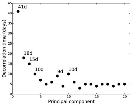
Figure 2: Decorrelation times (in days) of the 20 leading principal components.

The two-dimensional normalized histogram of $\textnormal{pc}_{1}$ and $\textnormal{pc}_{3}$ for the 500,000-day-long simulation is (cf. figure 3) similar to figure 7 in (Crommelin, 2003). To estimate the histogram, principal components $\text{pc}_{1}$ and $\text{pc}_{3}$ were normalized by their respective standard deviations and the $(\text{EOF}_{1},\text{EOF}_{3})$ plane was discretized into a grid $G$ of $50\times 50$ boxes spanning a $[-3,3]\times[-3,3]$ square. Grid boxes at the boundary are extended so that all realizations belong to the grid. Furthermore, if a box contains no realization, it is removed from the grid, as it is not likely to support part of the projection of the attractor. This resulted in a grid of $m=1577$ boxes containing on average $314$ realizations and such that $80\%$ of the boxes contain at least 20 realizations. The components $H_{i}$ of the normalized histogram $H$ for grid-box $B_{i}$ are then calculated as the likelihoods $\hat{\mathbb{P}}(y_{t}\in B_{i})=\#\{y_{t}\in B_{i}\}/\#\{y_{t}\in G\}$, where $\#\{y_{t}\in B_{i}\}$ is the number of realizations of the observable $\mathbf{y}$ in box $B_{i}$ and $\#\{y_{t}\in G\}$ is the total number of realizations.

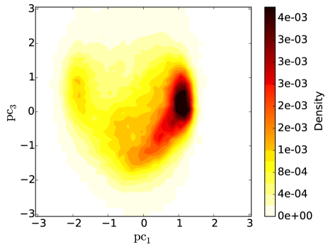
Figure 3: Normalized histogram of the first and third leading principal components normalized by their respective standard deviations and discretized using $50\times 50$ grid boxes.

The histogram in figure 3 shows two local maxima indicative of the presence of recurrent or persistent regimes. These regimes will be precisely defined in section IV.3. For now, following Crommelin (2003), we associate the local maximum for negative pc₁ to the blocked regime (since it corresponds to high pressure over north-western Europe) and the maximum for positive values of $\textnormal{pc}_{1}$ to the zonal regime. Crommelin (2003) also showed that the transitions from the zonal to the blocked regime were preferably going through negative values of $\textnormal{pc}_{3}$, interpreted as the positive phase of the NAO.

The dynamics of the state vector $\mathbf{x}$ of the barotropic model on the phase space $X$ are deterministic and Markovian. However, application of the Mori-Zwanzig formalism (Chorin and Hald, 2009; Darve et al., 2009; Kondrashov et al., 2015) indicates that in a closed model of the dynamics of the observable $\mathbf{y}$, memory terms accounting for past interactions between the resolved and the unresolved variables have to be included together with an, in general non-white, noise term. Under the assumption that the time scales of the resolved variables are slower by several orders of magnitude than those of the unresolved variables, these memory terms can be neglected (Givon et al., 2004; Majda et al., 2001). As can be seen in figure 2, the decorrelation time of the unresolved variables $\mathrm{pc}_{2}$ is not smaller that the one of the resolved variables $\mathrm{pc}_{1}$ and $\mathrm{pc}_{3}$ and hence time-scale separation does not apply and memory effects should be considered. In sections III and IV, we show how transfer operator techniques can provide detailed information on this issue.

III Transfer operators, resonances and their estimation

The spectrum of transfer operators giving the evolution of densities induced by the flow can provide valuable information on the time scales of the dynamics; in this section we show how these operators can be approximated on a reduced phase space.

III.1 Transfer operators of dissipative dynamical systems

We consider an autonomous dissipative dynamical system (DDS) governed by the ODE

$$\dot{\mathbf{x}}= F(\mathbf{x}), \quad\mathbf{x}\in X,$$ (4)

$$\mathbf{x}(0)= x_{0},$$

where $X=\mathbb{R}^{d}$ is an Euclidean vector space and $F:X\to X$ a smooth vector field with associated flow $\{S_{\tau}\}_{\tau\geq 0}$. The evolution of a distribution $f$ of $\mathcal{D}^{\prime}$ (Rudin, 1991) induced by the flow $\{S_{\tau}\}$ is described by a family of linear operators $\{\mathcal{L}_{\tau}\}_{\tau\geq 0}$, namely the Perron-Frobenius operators or transfer operators, such that

$$<\mathcal{L}_{\tau}f,g>=<f,g\circ\mathcal{S}_{\tau}>,\quad\text{for all }g\in\mathcal{C}^{\infty},$$ (5)

where $\circ$ is the composition operator and $<f,g>$ is the action of the distribution $f$ on the smooth function $g$. The family $\{\mathcal{L}_{\tau}\}_{\tau\geq 0}$ is a one-parameter semigroup, that is

$$\mathcal{L}_{\tau_{1}+\tau_{2}}=\mathcal{L}_{\tau_{1}}\mathcal{L}_{\tau_{2}}~{};~{}\mathcal{L}_{0}=I$$ (6)

While the more intuitive transfer operators acting on (integrable) probability densities (chap 7.4 in Lasota and Mackey, 1994) will be considered in section III.2 to V, it has been shown that the statistical properties, such as the decay rate of correlations, of several mixing dissipative systems are related to the point spectrum of transfer operators acting on (larger) spaces of distributions (Gouëzel and Liverani, 2006; Butterley and Liverani, 2007). Such statistics are provided by an ergodic invariant measure. A measure $\mu$ of a measurable space $(X,\mathcal{B}(X))$ is invariant under the flow $S_{\tau}$ if $\mu(S_{\tau}^{-1}(A))=\mu(A)$ for all sets $A$ in $\mathcal{B}(X)$. It is ergodic if all invariant sets $A$ are trivial subsets of $X$ ($\mu(A)=0$ or $\mu(A)=1$). Moreover, a dynamical system is mixing if $\lim_{t\to\infty}\mu(A\cap S_{\tau}^{-1}(B))=\mu(A)\mu(B)$, in which case the correlation function

$$\rho_{f,g}(\tau)=\int fg\circ S_{\tau}-\int f\int g\quad\text{for }f\in L^{1},g\in L^{\infty},$$ (7)

converges to zero as the lag $\tau$ goes to infinity (chap 4.4 in Lasota and Mackey, 1994).

In the case of a DDS for which the attractor has Lebesgue measure zero, it is important to choose a physical invariant measure for which spatial and temporal averages of continuous observables are identical for an initial set of positive Lebesgue measure (Eckmann and Ruelle, 1985; Young, 2002). It has been shown, for Anosov flows, that a physical measure of Sinaï-Ruelle-Bowen (SRB) type (Young, 2002) exists and that an appropriate Banach space $\mathfrak{B}$ can be defined on which the semigroup of transfer operators is bounded and strongly continuous (chap. 1.5, Engel and Nagel, 2001), with its point spectrum $P\sigma(\mathcal{L}_{\tau})$ located inside the complex unit-disk (Butterley and Liverani, 2007).

Whether the system considered in this study is Anosov is a difficult question. However, it has been observed that many-particle systems with sensitive dependence to initial conditions ”behave” as Anosov (Gallavotti and Cohen, 1995). We will follow this so-called chaotic hypothesis and assume that the transfer operators $\{\mathcal{L}_{\tau}\}_{\tau\geq 0}$ associated with the flow $\{S_{\tau}\}_{\tau\geq 0}$ constitute a strongly continuous semigroup and that there exists a unique SRB measure (i.e, 1 is the only eigenvalue of the transfer operators located on the unit disk, the system is mixing).

For a bounded and strongly continuous semigroup, there exists an infinitesimal operator $\mathcal{A}$, namely the generator of the semigroup, and $u(\tau)=\mathcal{L}_{\tau}f$ is the unique solution ($\forall\tau\geq 0$) of the following Cauchy problem (chap. 2.6 in Engel and Nagel, 2001)

$$\dot{u}(\tau)=\mathcal{A}u(\tau)~{};~{}u(0)=f.$$ (8)

For transfer operators, the linear system (8) is the Liouville equation which replaces the non-linear problem (4) at the expense of having to deal with a Partial Differential Equation (PDE).

The Spectral Mapping Theorem (SMT) (chap. 4.3.7, Engel and Nagel, 2001) allows us to relate the point spectrum $P\sigma(\mathcal{A})$ of the generator of a strongly continuous semigroup to the point spectrum $P\sigma(\mathcal{L}_{\tau})$ of the semigroup operators, according to

$$P\sigma(\mathcal{L}_{\tau})\setminus\{0\}=e^{\tau P\sigma(\mathcal{A})}.$$ (9)

A vector $\phi$ is called an eigenvector associated with the eigenvalue $\lambda$ in $P\sigma(\mathcal{L}_{\tau})$ if $\mathcal{L}_{\tau}\phi=\lambda\phi$.

The SMT will be used in section IV.1 to associate the spectrum of the transfer operators to motions of different time-scales. To fix the ideas, let us take an eigenvector $\phi$ (possibly a distribution) associated with a non-zero eigenvalue $\lambda$ of $P\sigma(\mathcal{L}_{\tau})$. For any observable $g$ (a smooth test function)

$$<\phi,g\circ S_{\tau}>= <\mathcal{L}_{\tau}\phi,g>$$ (10)

$$= \lambda<\phi,g>.$$ (11)

Applying the SMT, there exists an $\alpha$ in $P\sigma(\mathcal{A})$ such that $\lambda=e^{t\alpha}$, so that (11) becomes

$$<\phi,g\circ S_{\tau}>=e^{tRe(\alpha)}e^{itIm(\alpha)}<\phi,g>.$$ (12)

Thus, the term $<\phi,g\circ S_{\tau}>$ converges exponentially fast to zero at the rate $-Re(\alpha)>0$. Loosely speaking, the point spectrum of the generator $\mathcal{A}$ close to the imaginary axis (correspondingly, the point spectrum of $\mathcal{L}_{\tau}$ close to the unit circle) is responsible for a slow rate of decay of correlations in the direction of their eigenvectors. This point spectrum, called the Ruelle-Pollicott (RP) resonances (Pollicott, 1985; Ruelle, 1986a, b), is therefore a candidate for a mathematical explanation of the observed low-frequency variability such as induced by meta-stability. This important fact motivates the estimation of the RP resonances to study the dynamics associated with meta-stable regimes in section IV. In sections III.2 to IV, we present how these resonances can be calculated from approximations of the transfer operators on the reduced phase space.

III.2 Estimation of transfer operators on the reduced phase space

For Anosov systems, the stability of the SRB measure (Kifer, 1986; Dellnitz and Junge, 1999), the transfer operators (Blank et al., 2002) and the dominant part of their spectra (Keller et al., 1998; Baladi and Holschneider, 1999) to perturbations, has motivated the discrete approximation of transfer operators using Ulam-type methods (Dellnitz and Junge, 1999; Froyland, 2001; Blank et al., 2002; Chekroun et al., 2014).

For low-dimensional systems, Ulam’s method relies on a Galerkin approximation of the infinite-dimensional transfer operators by finite-dimensional matrices (Ulam, 1964; Froyland, 1998; Dellnitz and Junge, 1999). For this purpose, the phase space is discretized into a grid $G=\{B_{i}\}_{1\leq i\leq m}$ of $m$ grid boxes defining an orthogonal basis of characteristic functions. The transfer operator $\mathcal{L}_{\tau}$ is then approximated by a time-homogenous Markov chain with transition matrix $P_{\tau}$ whose elements are the transition probabilities

$$(P_{\tau})_{ij}=\mathbb{P}(x_{t+\tau}\in B_{j}|x_{t}\in B_{i}),$$ (13)

of a trajectory of $\mathbf{x}$ in box $B_{i}$ to pass through $B_{j}$ after a lag $\tau$. These probabilities can be estimated from a long time-series $\{x_{t}\}_{1\leq t\leq N}$ of $\mathbf{x}$ using the Maximum Likelihood Estimator (MLE)

$$(\hat{P}_{\tau})_{ij}=\hat{\mathbb{P}}(x_{t+\tau}\in B_{j}|x_{t}\in B_{i})=\frac{\#\{(x_{t}\in B_{i})\wedge(x_{t+\tau}\in B_{j})\}}{\#\{x_{t}\in B_{i}\}},$$ (14)

where $\#\{x_{t}\in B_{i}\}$ is the total number of realizations of $\mathbf{x}$ in $B_{i}$ and $\#\{(x_{t}\in B_{i})\wedge(x_{t+\tau}\in B_{j})\}$ is the number of realizations of $\mathbf{x}$ in box $B_{i}$ ending in $B_{j}$ $\tau$-time later. As $N$ goes to infinity, $(\hat{P}_{\tau})_{ij}$ converges to $(P_{\tau})_{ij}$ with an error of order $\mathcal{O}(N^{-1/2})$ (Billingsley, 1961).

Because, the high dimensionality of the phase space of the barotropic model ($d=231$) prohibits the direct approximation of $\mathcal{L}_{\tau}$ and because, as described in section II.2 and in Crommelin (2003), the dynamics relevant to transitions between meta-stable regimes predominantly occur in the reduced phase space $Y=(\mathrm{EOF}_{1},\mathrm{EOF}_{3})$, we instead estimate the transition probabilities of a Markov process associated with the dynamics in the reduced phase space $Y$ (Chekroun et al., 2014), by replacing $\mathbf{x}$ in (13) and (14) by the observable $\mathbf{y}=h(\mathbf{x})$. Markov operators approximated by these transition probabilities cannot be expected to give the transfer of densities in the reduced phase space as induced by the flow $S_{\tau}$. Nonetheless, it has been shown by Chekroun et al. (2014, Theorem A), for systems with a unique SRB measure and a continuous observable $h$, that the transition probabilities in the full phase-space $X$, are related to the transition probabilities of the Markov process on the reduced phase-space $Y$ by

$$\mathbb{P}(y_{t+\tau}\in B_{j}|y_{t}\in B_{i})=\mathbb{P}(x_{t+\tau}\in h^{-1}(B_{j})|x_{t}\in h^{-1}(B_{i})).$$ (15)

Hence the transition probabilities in $X$ restricted to pairs $(h^{-1}(B_{i}),h^{-1}(B_{j}))$ are exactly the transition probabilities in $Y$ for pairs $(B_{i},B_{j})$. As a consequence, the estimated transition matrices $\{\hat{P}_{\tau}\}$ contain information on the transfer operators $\{\mathcal{L}_{\tau}\}$ and their RP resonances as filtered by the observable.

Accordingly, we have discretized the reduced phase space $Y$ using exactly the same $50\times 50$ grid as for the histogram as in section II.2. Then, the matrices $\{\hat{P}_{\tau}\}$ were estimated from the 500,000-day-long time-series of $\mathbf{y}$ and for different lags $\tau$. Importantly, $\{\hat{P}_{\tau}\}_{\tau\geq 0}$ need not be a semigroup because (i) the partial observation of the system introduces memory effects (Darve et al., 2009; Chorin and Hald, 2009), (ii) the Galerkin approximation adds numerical diffusion (Froyland et al., 2013) and (iii) the estimation of transition probabilities from a time-series of limited length is prone to sampling errors (cf. section IV below).

Before to study in detail the spectral properties of the transition matrices, we remark that these matrices are row stochastic, implying that their eigenvalues satisfy $|\lambda|\leq 1$. In our case, there exists necessarily a unique eigenvalue equal to $1$ because the transition matrices $\{\hat{P}_{\tau}\}$, by construction from a unique time series, represent irreducible Markov chains (Baladi, 2000). The uniqueness of this eigenvalue in turn implies that its associated eigenvector $\vec{\pi}=\{\pi_{1},...,\pi_{m}\}$, or fixed point, is in fact identical to the normalized histogram $H$ of figure 3.

Indeed the following calculation shows that the histogram $H$ is invariant for any $\hat{P}_{\tau}$

$$(H\hat{P}_{\tau})_{j}= \sum_{k=1}^{m}H_{k}(\hat{P}_{\tau})_{kj}$$

$$= \sum_{k=1}^{m}\frac{\#\{y_{t}\in B_{k}\}}{\#\{y_{t}\in G\}}\times\frac{\#\{(y_{t}\in B_{k})\wedge(y_{t+\tau}\in B_{j})\}}{\#\{y_{t}\in B_{k}\}}$$

$$= \sum_{k=1}^{m}\frac{\#\{(y_{t}\in B_{k})\wedge(y_{t+\tau}\in B_{j})\}}{\#\{y_{t}\in G\}}$$

$$= \frac{\#\{y_{t+\tau}\in B_{j}\}}{\#\{y_{t}\in G\}}$$

$$= H_{j}.$$

Thus, each component $\pi_{i}$ yields the likelihood $\hat{\mathbb{P}}(y_{t}\in B_{i})$ for realizations of the observable to be in $B_{i}$. It is straightforward to associate to any m-dimensional vector on the grid $G$ the corresponding density it approximates (Froyland and Padberg, 2009). Not doing the distinction between a probability vector and the corresponding probability density should thus not lead to any confusion.

IV Spectral properties, memory and almost-invariant sets

IV.1 Spectral properties and slow dynamics

We now apply the Spectral Mapping Theorem (SMT) in order to approximate the RP resonances (the dominant eigenvalues of the generator) from the estimated transition matrices $\hat{P}_{\tau}$, as filtered by the observable $h$. For this purpose, we first solve, for each estimated transition matrix in $\{\hat{P}_{\tau}\}$, the eigenvalue problem

$$\vec{e}_{i}(\tau)\hat{P}_{\tau}=\lambda_{i}(\tau)\vec{e}_{i}(\tau)\quad\text{for }i\in\{1,...,m\},$$ (16)

where $\vec{e}_{i}(\tau)$ is the left-eigenvector associated with the $i^{th}$ eigenvalue $\lambda_{i}(\tau)$ of $\hat{P}_{\tau}$. The spectrum of $\hat{P}_{\tau}$ changes with the lag $\tau$. However, if $\{\hat{P}_{\tau}\}_{\tau\geq 0}$ was a semigroup with generator $\mathcal{A}_{m}$, the spectrum $\{\alpha_{i}\}$ of $\mathcal{A}_{m}$ would be independent of $\tau$ and applying the SMT would give

$$r_{i}=-Re(\alpha_{i})=-\frac{1}{\tau}\log{|\lambda_{i}(\tau)|}\quad\text{for }\tau>0\text{ and for }i\in\{1,...,m\},$$ (17)

where $r_{i}$ would be the exponential rate of decay of correlation of any observable in the reduced phase-space with the eigenvector associated with $\lambda_{i}$.

However, as noted section III.2, the transition matrices $\{\hat{P}_{\tau}\}_{\tau\geq 0}$ do not necessarily inherit from the semigroup property (6) of the transfer operators $\{\mathcal{L}_{\tau}\}_{\tau\geq 0}$. Thus, no generator may exist and the rates $r_{i}$ in (17) may depend on the lag $\tau$. Nevertheless, calculating the rates $r_{i}(\tau)$ for each lag allows (i) to give an approximation of the dominant RP resonances with a control on the lag and (ii) to test the semigroup property (6).

For this purpose, we calculated the rates $r_{i}(\tau)$ by solving the eigenvalue problem (16) and applying (17) for $\tau$ ranging from 1 to 39 days. The leading rate equals $0$, since it is associated to the unit-eigenvalue. The rates corresponding to the 10 leading eigenvalues different from unity of each $\hat{P}_{\tau}$ are represented figure 4 with the lag $\tau$ as abscissa and the (cyclic) coloring distinguishing the rank of the rate. A complex pair of conjugate eigenvalues is represented by one square for the two conjugates. The error bars represent $99\%$ confidence intervals estimated from a thousand surrogate transition matrices by applying the bootstrap method described in Appendix A.

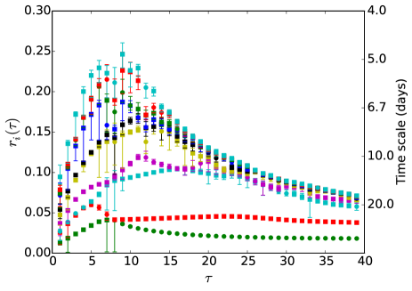
Figure 4: Rates $r_{i}(\tau)$ corresponding to the 10 leading eigenvalues different from unity of each $\hat{P}_{\tau}$, with the lag $\tau$ as abscissa and the (cyclic) coloring giving the rank of the rate. A complex pair of eigenvalues is represented by one square for the two conjugates. The error bars represent $99\%$ confidence intervals estimated from a thousand surrogate transition matrices by applying the bootstrap method described in Appendix A.

Our first observation concerns the small width of the confidence intervals (some are even hidden by the marker size). These intervals evaluate the robustness of the estimates to the limited length of the time-series. The largest intervals occur when two rates almost overlap, so that one of them may appear or disappear in the surrogates, resulting in a change of rank for all higher-rank rates. In our case, large confidence intervals are thus usually indicative of an uncertainty in the existence of two close but distinct rates or of only one (as for the leading rates at $\tau=7$ or $8$, for example). Moreover, Appendix A shows that at least the three leading rates are very robust to changes in the the grid resolution, ranging from a $10\times 10$ grid to a $100\times 100$ grid, compared to the original $50\times 50$ grid.

Being confident on the robustness of the rates to the sampling as well as to the grid resolution, we now turn to a detailed analysis of the results in figure 4. First, we can see that the two rates closest to zero, the leading rates in red and green, are well separated from the rest of the spectrum after a lag between 5 and 10 days. One of these rates derives from a real eigenvalue (the circle), the other represents a pair of complex conjugate eigenvalues (the square); they exchange rank at a lag of 8 days. We can calculate an indicative time scale associated with each rate as the inverse of the rate. Whether this time scale corresponds, to a good approximation, to a decorrelation time is not the matter of this study. For a lag of 15 days, the first rate (in green) and the second rate (in red) correspond to a time scale of $40$ and $23$ days respectively. Furthermore, the second rate is separated from the third (in cyan) by a gap of 13 days. This time-scale separation suggests that the reduced dynamics are slowly mixing due to the presence of meta-stable regimes responsible for low-frequency variability (Dellnitz and Junge, 1997; Froyland and Dellnitz, 2003; Chekroun et al., 2014). This confirms the work on meta-stable atmospheric regimes in this model by Crommelin (2003); we will see in section IV.3 how such regimes can be more objectively detected.

The second important feature, relevant to the problem of stochastic prediction of section V.2, is the relative constance of the two leading rates for lags larger than $8$ days. We can say that the slow dynamics associated with these rates ”behave as Markovian”, by which we mean that looking only at these rates, one cannot disprove the semigroup property (6), even though the dependance on the lag of the other rates is clearly indicative that $\{\hat{P_{\tau}}\}_{\tau\geq 0}$ cannot constitute a semigroup. Thus, the two leading rates do not seem to be affected by memory effects due to the partial observation of the system or by estimate errors, since one would not expect them to be constant otherwise.

From the separation of the two leading rates from the other rates as well as their relative independence on the lag $\tau$ for lags larger than $8$ days, we expect $8$ days to be the minimum lag for which the transition matrix $\hat{P}_{\tau=8}$ is likely to predominantly resolve the dynamics associated with the meta-stable regimes. Consequently, the following developments will rely mostly on the transition matrix $\hat{P}_{\tau=8}$. Such strategy for the choice of the lag is similar to the one of DelSole (2000) and Berner (2005), who look directly at the decorrelation rate of their time series to infer for which lag they should estimate the drift and diffusion coefficients of the Fokker-Planck equation they want to approximate. In our case, however, all the rates associated with the dominant eigenvalues of the transfer operators are considered and not only the decorrelation rate of the time series alone. Let us also acknowledge that the SMT has been used in Crommelin and Vanden-Eijnden (2011) to estimate the spectrum of the generator associated with a Fokker-Planck equation, in Froyland et al. (2013) to compare approximates of transfer operators and generators of low-dimensional dynamical systems and in Franzke et al. (2008) to test the meta-stability of Hidden Markov Models. However, we do not know other studies using the SMT to test the ”Markovianity” of reduced systems, even though the $\tau$-test in Penland and Sardeshmukh (1995) serves a similar purpose in the context of Linear Inverse Modeling.

IV.2 Further validation of the semigroup property

We further test to which extent the semigroup property (6) is violated for special cases of powers $k$ of $\hat{P_{\tau}}$ and the corresponding matrices $\hat{P}_{k\times\tau}$. Rather than directly calculating a distance between the matrices $(\hat{P}_{\tau})^{k}$ and $\hat{P}_{k\times\tau}$, we prefer to calculate, for an initial density $f_{0}$, the distance between the density $f_{k\tau}^{\mathrm{pow}}=f_{0}(\hat{P_{\tau}})^{k}$ transferred by the $k^{th}$ power of $\hat{P_{\tau}}$ and the density $f_{k\tau}^{\mathrm{long}}=f_{0}\hat{P}_{k\times\tau}$ transferred by $\hat{P}_{k\times\tau}$. We use the distance $d(f,g)=\sqrt{\sum_{i=1}^{m}\pi_{i}(f_{i}-g_{i})^{2}}$, which is a sum of squared errors between the components of $f$ and $g$, weighted by the likelihoods $\hat{\mathbb{P}}(y_{t}\in B_{i})$, so that errors in grid boxes less likely to be reached by the Markov process are given less weight. The distances $d(f_{k\tau}^{\mathrm{pow}},f_{k\tau}^{\mathrm{long}})$ have been calculated for a set of $m$ initial densities associated with each grid-box in $\{B_{i}\}$, so that the density associated with box $B_{j}$ integrates to 1 in $B_{j}$ and to zero elsewhere. The distances are represented figure 5a and b for a lag $\tau$ of 8 days and for a multiplicator $k$ of $2$ and $4$, respectively (dark colors indicate small distance).

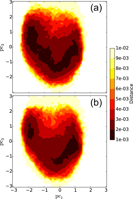
Figure 5: The value at each grid-point represents the distance, for an initial density of 1 at this grid-point, between the density $f_{8k}^{\mathrm{pow}}$ transferred by the $k^{th}$ power of $\hat{P_{8}}$ and a density $f_{8k}^{\mathrm{long}}$ transferred by $\hat{P}_{k\times 8}$ for (a) $k=2$ and (b) $k=4$.

To explain the nature of the violation of the semigroup property (6), let us recall that there exists only three possible candidates, namely (i) the partial observation of the dynamical system, (ii) the coarse-graining induced by the Galerkin approximation and (iii) sampling errors. Furthermore, it is shown in Appendix B, that the distances plotted figure 5 are not affected by the use of twice as more samples and that they only decrease slightly when the resolution increases (and vice versa). Thus, we can say that positive distances in figure 5 are mostly the consequence of memory effects induced by the partial observation of the high-dimensional barotropic model.

We can observe that these memory effects are mostly important where the stationary density is small (figure 3) and thus, where trajectories are less likely to pass by. The denser regions which are associated with meta-stability, as will be seen section IV.3, seem to be less affected by memory effects. This result is in agreement with the relative constancy with lag of the leading rates, also associated with meta-stability. Such memory effects, as well as the dependence on the lag of the spectral gap between the leading rates, should be put in perspective with stochastic modeling with Stochastic Differential Equations (SDE) and based on time-scale separation (Majda et al., 1999, 2001; Franzke et al., 2015). Indeed, in such models, one seeks a reduced basis for the decorrelation time of the resolved variables to be much longer than the one of the unresolved variables, in order to be able to neglect the memory effects made explicit by the Mori-Zwanzig formalism (Darve et al., 2009; Chorin and Hald, 2009). If the transition matrices on the reduced phase space do not directly help in the choice of the basis on which the dynamical system can be optimally reduced, their rates can give insights on the impact of the reduction on the resolved variables.

IV.3 Meta-stable regimes as almost-invariant sets of the transfer operator

We have seen, section IV.2, that the two leading rates of figure 4 are close to zero and that a large spectral gap separates them from the rest of the rates, a configuration indicative of the presence of meta-stable regimes. This characteristic of meta-stability or persistence allows to formally define these regimes as almost-invariant sets (Dellnitz and Junge, 1997; Froyland and Dellnitz, 2003). We now give an extension of the definition of almost-invariant sets to sets in the reduced phase space and present an algorithm to detect them from a transition matrix $\hat{P}_{\tau}$.

A set $A$ of the phase space $X$ is almost-invariant if $S_{\tau}^{-1}(A)\approx A$, so that

$$\mathbb{P}(x_{t+\tau}\in A|x_{t}\in A)\approx 1.$$ (18)

Reformulating, the probability for a trajectory starting in a set $A$ to leave this set after a lag $\tau$ is almost-zero. These sets are thus associated with persistent or meta-stable regimes.

In the case of almost-invariant sets in the reduced phase space, we are interested in sets $E$ of $Y$, almost-invariant with respect to the transition probabilities $\mathbb{P}(y_{t+\tau}\in E|y_{t}\in E)$, such that

$$\mathbb{P}(y_{t+\tau}\in E|y_{t}\in E)\approx 1.$$ (19)

However, applying (15) (Chekroun et al., 2014, Theorem A) we have that

$$\mathbb{P}(y_{t+\tau}\in E|y_{t}\in E)\approx 1\quad\iff\quad\mathbb{P}(x_{t+\tau}\in h^{-1}(E)|x_{t}\in h^{-1}(E))\approx 1.$$ (20)

This important result states that if a set $E$ is almost-invariant in the reduced space $Y$, its pre-image $h^{-1}(E)$ in $X$ is almost-invariant to the flow $S_{\tau}$. In other words, almost-invariant sets in the reduced phase space are images of almost-invariant, yet coarser, sets in the full phase space. Of course, these coarse-grained almost-invariant sets may not be optimal, in the sense that other, more strongly almost-invariant sets (w.r.t (19)) may exist but are filtered out by the observable $h$ in the same way RP resonances can be filtered out by $h$.

Based on these considerations, the transition matrix $\hat{P}_{\tau=8}$ was used to define the meta-stable regimes objectively. For the detection of almost-invariant sets (see also, Dellnitz and Junge, 1997; Froyland and Dellnitz, 2003; Froyland and Padberg, 2009) we use an optimal Markov chain reduction (Deng et al., 2011; Rosvall and Bergstrom, 2008) with respect to the relative entropy rate Cover and Thomas (1991). This type of Markov chain reduction is particularly well suited for the detection of dense almost-invariant sets (highly recurrent), since it attempts to minimize the distance between a density transferred by the reduced transition matrix (giving the transition probabilities between the almost-invariants, see below) and the same density transferred by the original transition matrix. The optimization was implemented using the greedy algorithm from network theory (Clauset et al., 2004), where the grid-boxes are iteratively merged to give coarser and coarser almost-invariant sets.

In accordance with the bimodality of the histogram (figure 3), we have chosen to look for a number of almost-invariant sets $p$ of 2. These two sets are plotted in figure 6, such that all grid boxes in green belong to the first almost-invariant set and all grid boxes in blue belong to the second one. For the family of almost-invariant sets $\{E_{\beta}\}$, the 2-by-2 reduced transition matrix $\hat{Q}_{\tau=8,}$, such that $(\hat{Q}_{\tau=8})_{\beta\gamma}=\hat{\mathbb{P}}(y_{t+\tau}\in E_{\gamma}|y_{t}\in E_{\beta})$, and its stationary density $\eta$, such that $\eta_{\beta}=\hat{\mathbb{P}}(y_{t}\in E_{\beta})$, are found to be

$$\hat{Q}_{\tau=8}=\begin{pmatrix}0.79&0.21\\ 0.14&0.86\end{pmatrix},\quad\eta=\begin{pmatrix}0.27\\ 0.73\end{pmatrix},$$ (21)

the second almost-invariant set (in blue) being almost three times as dense as the first one (in green).

The algorithm is designed to find almost-invariant sets whose union covers the entire grid. However, in view of the early warning problem discussed in section V, we need to find a restriction of the definition of the regimes $\{R_{\beta}\}$ to smaller regions of the grid so that the likelihood $\hat{\mathbb{P}}(y_{t}\in R_{\beta})$ to be in any regime $R_{\beta}$ becomes smaller than one Kharin and Zwiers (2003). To do so, we selected, for each almost-invariant set $E_{\beta}$, their grid-boxes $B_{i}$ maximizing the likelihood $\hat{\mathbb{P}}(y_{t}\in B_{i},y_{t+\tau}\in E_{\beta},y_{t-\tau}\in E_{\beta})$ of a realization of $\mathbf{y}$ to be in $B_{i}$ and to come from and go to the same almost-invariant set $E_{\beta}$, until a sufficiently large number of boxes have been attributed to the regime $R_{\beta}$ to have $\hat{\mathbb{P}}(y_{t}\in R_{\beta})=\hat{\mathbb{P}}(y_{t}\in E_{\beta})/2$ (until half of the almost-invariant set has been selected in terms of stationary density $\pi$). These restrictions are plotted in dark green and dark blue (Fig. 6) and define the blocked and zonal regimes, respectively. The probability to stay in the so-defined blocked and zonal regimes after 8 days is of $66\%$ and $70\%$, respectively.

It is shown in the Appendices A, B and C that these regimes are relatively robust to the limited length of the time series, to the grid resolution and to the lag, respectively. Their definition together with the transition matrices $\{\hat{P}_{\tau}\}$ are used in section V to define an early warning indicator of a transition to the blocking regime.

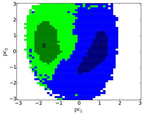
Figure 6: Two almost-invariants sets and their restrictions (in dark colors) corresponding to the blocked and the zonal regime, respectively.

V Preferred transition paths and early warning

V.1 Preferred transition paths

Having defined the regimes, we now study the transitions between them. Following Branstator and Berner (2005), we first plot the mean tendencies of the normalized principal components pc₁ and pc₃. The tendencies were calculated for each principal component using a finite difference scheme such that $\Delta\text{pc}_{i}(t)=(\text{pc}_{i}(t+\Delta t)-\text{pc}_{i}(t))/\Delta t$, where $\Delta\text{pc}_{i}$ is the approximate tendency of the $i^{th}$ principal component and $\Delta t$ is the time step. An estimate of the mean tendency for each grid box was then calculated by averaging over all the realizations of $\mathbf{y}$ in this grid box.

The mean tendency for a time-step $\Delta t$ of 8 days is plotted figure 7. It can be seen as a composition of a clockwise rotation and two sinks. This result corroborates both the meta-stability of the regimes and the existence of preferred transition paths between them, reminiscent of a pseudo-periodic orbit (Plaut and Vautard, 1994; Crommelin, 2003). Indeed, the rotation is such that typical trajectories leaving the zonal regime (blocked regime) to go to the blocked regime (zonal regime) transit through negative values (positive values) of pc₃. Furtermore, the correspondence between the sinks with low-values of mean tendency and the regimes is striking, in particular for the zonal regime. We have seen in section IV.2 that the memory effects are relatively weak in the region of the regimes. In the limit when these effects can be neglected, the reduced dynamics can be modeled by an SDE and the mean tendency gives an approximation of the drift term involved in the Fokker-Planck equation (together with diffusion, not calculated here, Berner, 2005; Gardiner, 2009) which generates the semigroup of transfer operators associated with the SDE. The correspondence between weak tendency and almost-invariance is thus not coincidental.

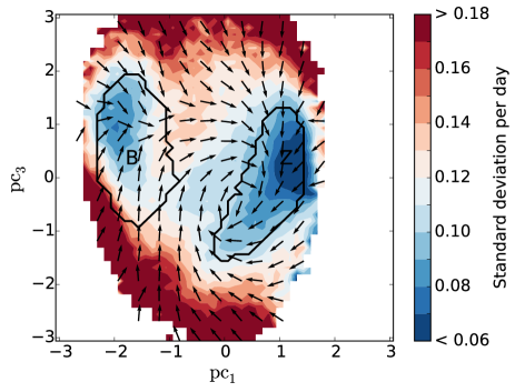
Figure 7: Mean tendency of the normalized principal components calculated using centered differences for $\Delta t=8$ days. Arrows represent the direction and the colors represent the magnitude (in standard deviation per day). As for the following figures, the black contours delimitate the blocked regime, marked by the letter B, and the zonal regime, marked by the letter Z.

To further support the existence of preferred transition paths from one regime to the other, we have calculated, for each grid box, the likelihood $\hat{P}_{ZB}$ ($\hat{P}_{BZ}$) that a trajectory starting in the zonal regime (blocked regime) and passing through this grid box reaches the blocked regime (zonal regime) before the zonal regime (blocked regime).

The resulting likelihoods are plotted in figure 8. In agreement with the tendency, the trajectories going from the zonal to the blocked regime are more likely to do so through low values of the $3^{rd}$ principal component while trajectories going from the blocked to the zonal regime favor high values of the $3^{rd}$ principal component.

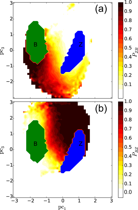
Figure 8: Likelihood, for each grid box, to reach (a) the blocked regime before the zonal regime and (b) the zonal regime before the blocked regime.

V.2 Early warning indicator

The presence of preferred transition paths from the zonal to the blocked regime, as well as the weak mixing associated with the existence of rates close to zero (cf. section IV.1), suggests that there is potential skill in predictability of transitions to the blocked regime. Note that more than trying to predict when a trajectory will leave the zonal regime, we want to use the fact that trajectories leaving the zonal regime are more likely to go to the blocked regime if they transit through negative values of pc₃. We therefore use the transition matrices for different lags to provide an approximation of the transfer of densities in the reduced phase space by the flow and to build an early-warning indicator of transitions to the blocked regime.

The quality of the indicator will depend on (i) the predictability of the full system (in terms of sensitive dependence to initial conditions or rate of decay of correlations) and (ii) the validity of the Markov approximation for the reduced dynamics. While the former is determined by the dynamical system alone, the latter depends on the choice of the observable. We have seen in section IV that the violation of the semigroup property indicates that the reduced dynamics are overall non-Markovian. However, the constancy of the leading rates also indicates that motions associated with the meta-stable regimes behave as Markovian, suggesting that densities transferred by the estimated transition matrices could be used to give a probability of reaching one of the regimes.

The early-warning indicator is thus designed as such. Whenever the observed trajectory (in our case, the simulation) leaves the zonal regime, we define an initial density $f_{B_{i},\tau=0}$, integrating to 1 over grid-box $B_{i}$ to which the last observation belongs and to zero elsewhere (one could instead define an initial density spreading over several boxes to account for uncertainties in the observation). Next, the Markov approximation $f_{B_{i},\tau=1}$ of the transfer of $f_{B_{i},\tau=0}$ by the flow after a lag $\tau$ of 1 day is calculated as $f_{B_{i},\tau=0}\hat{P}_{\tau=1}$. We then calculate the likelihood $\hat{\mathbb{P}}(y_{\tau=1}\in R_{\mathrm{block}}|y_{0}\in B_{i})=\sum_{B_{j}\in R_{\mathrm{block}}}(f_{B_{i},\tau=1})_{j}$ for a realization $y_{t+1}$ to belong to the blocking regime knowing that $y_{t}$ belongs to grid-box $B_{i}$. If this estimated probability exceeds a given critical probability $p_{c}$, an alarm of transition to the blocked regime after a lag $\tau_{\mathrm{alarm}}$ of 1 day is given. Otherwise, the same process is repeated for $\tau=2,3,...$ until an alarm is given or a limit lag $\tau_{\mathrm{max}}$ is reached, after which we wait for the next observation to run the forecasting system.

To illustrate this process we show in figure 9 the transferred density for grid box 314 marked as a blue square and lying in the region of preferred transition paths between the zonal and the blocked regimes. This initial density $f_{B_{i=314},\tau=0}$, is plotted alone panel d). The densities $f_{B_{i=314},\tau=4}$, $f_{B_{i=314},\tau=8}$ and $f_{B_{i=314},\tau=16}$ transferred using the transition matrices $\hat{P}_{\tau=4}$, $\hat{P}_{\tau=8}$ and $\hat{P}_{\tau=16}$ are plotted panel (a), (b) and (c), respectively. The densities $f_{B_{i=314},\tau=2\times 4}$ and $f_{B_{i=314},\tau=2\times 8}$ transferred using the square of the transition matrices $\hat{P}_{\tau=4}$ and $\hat{P}_{\tau=8}$ are also plotted panel e) and f), respectively, to show how the semigroup property can be violated. The corresponding likelihoods to reach the blocked regime are written in the top left of each panel.

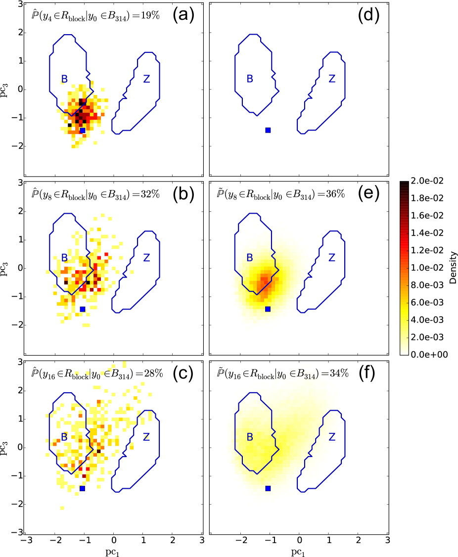
Figure 9: Markov approximation $f_{B_{i=314},\tau}$ of the transfer of the initial density $f_{B_{i=314},\tau=0}$ for a lag $\tau$ of (a) 4 days, (b) 8 days and (c) 16 days. The initial density is plotted in panel (d), integrating to one over box $B_{i=314}$ and to zero elsewhere. The densities transferred using the square of $\hat{P}_{\tau=4}$ and of $\hat{P}_{\tau=8}$ are plotted panel (e) and (f), respectively. The corresponding likelihoods to reach the blocked regime are written in the top left of each panel.

We can see that if a critical probability $p_{c}$ of 0.3 would be chosen, an alarm of transition to the blocking regime would be raised for $\tau=8$ days (figure 9b), as described in the previous paragraph. Figure 10 shows the grid boxes for which an alarm would be given if a critical probability $p_{c}$ of 0.3 was used and the respective lag $\tau_{\mathrm{alarm}}$ after which the transition is predicted to occur. In this case, alarms are mainly flagged for trajectories passing through grid boxes close to the blocked regime or in the region of low principal component pc₃.

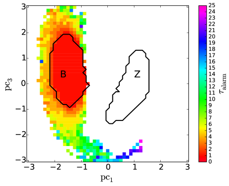
Figure 10: Predicted time of transition to the blocked state $\tau_{\mathrm{alarm}}$, in days, for each grid box where an alarm is given for a critical probability $p_{c}$ of 0.3.

The quality of the early warning indicator of transition to the blocked regime was tested over all trajectories starting when leaving the zonal regime and ending when reaching any of the regimes. In order to take into account sampling errors in the estimation of the transition matrices, the test was performed on a second $500,000$-day-long simulation which was ran taking as initial state the last state of the original simulation from which the transition matrices were estimated. Out of the $11759$ trajectories starting from the zonal regime, $1993$ reached the blocked regime, which we call an occurrence event (O), while $9766$ reached the zonal regime, which we call a non-occurrence event ($\overline{\text{O}}$).

When testing a forecast system, one is interested in how many alarms (A) were given when the event actually occurred, the number of so-called hits, and how many did not occur, the number of so-called false alarms. In the case of a hit, the event occurs at a given time $\tau_{\mathrm{occ}}$ after the alarm is given, so that not only the occurrence of the event should be forecasted, but also when it will occur. For easy reference, the different cases are shown in Table 1. For example, a forecast that a blocking event will occur in a month although it will truly occur only a week later is not of much help. For the purpose of assessing the skill of a forecast not only in terms of occurrence but also in terms of precision of the forecasted date of occurrence, we need to define a tolerance $\epsilon$, in days, such that a hit (H) is granted only when an alarm is given with a prediction time $\tau_{\mathrm{alarm}}$ such that $\tau_{\mathrm{occ}}-\epsilon\leq\tau_{\mathrm{alarm}}\leq\tau_{\mathrm{occ}}+\epsilon$. If, however, the event is predicted to happen too early ($\tau_{\mathrm{alarm}}<\tau_{\mathrm{occ}}-\epsilon$), it is counted as a false alarm of type II (FA2), while if the event is predicted to happen too late ($\tau_{\mathrm{alarm}}>\tau_{\mathrm{occ}}+\epsilon$), it is counted as a missed alarm of type II (MA2). When the event did not occur and no alarm ($\overline{\text{A}}$) was given, we count a correct rejection (CR). When an event occurs but no alarm is given, we count a missed alarm of type I (MA1) and when an event is predicted but does not occur, we count a false alarm of type I (FA1).

Table 1: Overview of the different cases which can occur depending on the alarm given and the event occurring.

	A	A	A	$\overline{\text{A}}$
	$\tau_{f}<\tau_{o}-\epsilon$	$|\tau_{f}-\tau_{o}|\leq\epsilon$	$\tau_{f}>\tau_{o}+\epsilon$
O	FA2	H	MA2	MA1
$\overline{\text{O}}$	FA1	FA1	FA1	CR

To assess the skill of the forecasts based on the categories defined in Table 1, we adapted the original Peirce skill score (PSS) (Peirce, 1884; Stephenson, 2000) to forecasts including the time of occurrence. In our case, we define the PSS as

$$S_{Peirce}(p_{c})=\text{HR}(p_{c})-\text{FAR}_{1}(p_{c}),$$

where $\text{HR}(p_{c})=\text{H}(p_{c})/\text{O}(p_{c})$ is the hit rate, defined as the ratio of the number of hits over the number of occurrences, and $\text{FAR}_{1}(p_{c})=\text{FA1}(p_{c})/\overline{\text{O}}(p_{c})$ is the false alarm rate of type I. The hit rate gives the likelihood of giving an alarm when the event occurs, while the false alarm rate of type I gives the likelihood that an alarm is given but the event does not occur. If the hit rate exceeds the false alarm rate the PSS is positive and the forecast has skill. A PSS of 1 is reached for a perfect forecast, when alarms are only raised when an event will actually occur and with the right predicted time of occurrence.

The PSS is plotted figure 11 versus the critical probability $p_{c}$ and for different tolerances $\epsilon$. A tolerance of $\infty$ means that the precision of the predicted date of occurrence is not taken into account in the skill score. It is evident that as the tolerance increases, the skill score increases as well. The PSS reaches a maximum for a critical probability around 0.5, depending on the tolerance. Such scores have to be put in perspective with the predicted time of occurrence $\tau_{\mathrm{alarm}}$. Indeed, a successful prediction of occurrence of a blocking event $1$ day ahead is counted as a hit, but is not of much practical use. For this reason, we have also represented the average prediction time $\tau_{\mathrm{alarm}}$ as a black dashed line on the same figure 11. It is of around two weeks for a critical probability of 0.3 and around one week for a critical probability of 0.45. Thus, depending on the final purpose of the forecast system, a compromise has to be found between the skill of the forecast system and how many days ahead an event is predicted on average. Choosing a critical probability of 0.3 would give a reasonably good skill score of 0.4 (better than a no-skill forecast) with an average prediction time of 2 weeks.

To summarize, the main advantage of a forecast system relying on the transfer of densities is that it constitutes a very cheap way to account for the sensitive dependence on initial conditions of a chaotic dynamical system.

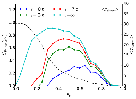
Figure 11: Peirce skill score of the probability forecast of reaching the blocked regime versus the critical probability $p_{c}$ for different tolerances $\epsilon$ (straight lines). The average time lag in days for which an alarm is given is also plotted in black dashed line.

VI Energetics of the transitions

In this section we focus on the remaining question on how the dynamics of the barotropic model can explain (i) the persistence of each regime and (ii) the preferred transition paths from the zonal to the blocked regime through high values or $\textnormal{pc}_{3}$.

To help clarifying these issues the hemispheric energy budget of the model is studied. First, the fields are decomposed in a $\bar{\tau}=8$ days running mean and a deviation from it. This decomposition yields for the streamfunction

$$\begin{split}\psi&=\overline{\psi}+\psi^{\prime}\quad\text{with}\quad\overline{\psi}=\frac{1}{\bar{\tau}}\int_{t-\bar{\tau}/2}^{t+\bar{\tau}/2}\psi~{}dt^{\prime}.\end{split}$$ (22)

Inserting (22) into equation (1)and applying the running mean gives the equation of the mean relative vorticity

$$\frac{\partial{\nabla^{2}\overline{\psi}}}{\partial{t}}+\mathcal{J}(\overline{\psi},\nabla^{2}\overline{\psi}+f+h)+\overline{\mathcal{J}(\psi^{\prime},\nabla^{2}\psi^{\prime})}=-k_{1}\nabla^{2}\overline{\psi}+k_{2}\nabla^{8}\overline{\psi}+\nabla^{2}\psi^{*}.$$ (23)

Subtracting (23) from (1) gives the equation of the deviation from the running mean as

$$\frac{\partial{\nabla^{2}\psi^{\prime}}}{\partial{t}}+\mathcal{J}(\overline{\psi},\nabla^{2}\psi^{\prime})+\mathcal{J}(\psi^{\prime},\nabla^{2}\overline{\psi}+f+h)$$

$$+\mathcal{J}(\psi^{\prime},\nabla^{2}\psi^{\prime})-\overline{\mathcal{J}(\psi^{\prime},\nabla^{2}\psi^{\prime})}=-k_{1}\nabla^{2}\psi^{\prime}+k_{2}\nabla^{8}\psi^{\prime}.$$ (24)

In order to obtain the equation of the hemispheric average of the mean kinetic energy $\overline{E}=<\frac{\overline{u}^{2}+\overline{v}^{2}}{2}>$, with $<\cdot>$ denoting the hemispheric average $\frac{1}{2\pi}\int_{0}^{2\pi}\int_{0}^{\pi/2}\cdot\cos\phi\textnormal{d}\phi\textnormal{d}\lambda$, equation (23) is multiplied by $\overline{\psi}$ and averaged hemispherically, giving

$$\frac{\partial\overline{E}}{\partial{t}}=<\overline{\psi}\text{ }\overline{\mathcal{J}(\psi^{\prime},\nabla^{2}\psi^{\prime})}>-2k_{1}\overline{E}-k_{2}<\overline{\psi}\nabla^{8}\overline{\psi}>-<\overline{\psi}\nabla^{2}\psi*>.$$ (25)

The first term on the right hand side is equal to the opposite of the sum of the Reynolds’ stress terms which represent a conversion of mean to eddy kinetic energy. Finally, multiplying (24) by $\psi^{\prime}$, applying the running mean and averaging over the hemisphere gives the equation of the global eddy kinetic energy $E^{\prime}=<\frac{\overline{u^{\prime 2}}+\overline{v^{\prime 2}}}{2}>$

$$\frac{\partial E^{\prime}}{\partial t}=-<\overline{\psi}\overline{\mathcal{J}(\psi^{\prime},\nabla^{2}\psi^{\prime})}>-2k_{1}E^{\prime}-k_{2}<\psi^{\prime}\nabla^{8}\psi^{\prime}>.$$ (26)

The terms in the equations (25) and (26) were calculated from the model simulation results and we could verify that the calculated tendencies equated the sum of the right hand side terms but for a small error of up to $13\%$ of the standard deviation of the tendencies due to the running average of a deviation not being exactly zero.

The energetics of the transitions can be studied by plotting the kinetic energies (Fig. 12) and the terms in the energy budget (Fig. 13) averaged for each grid box of the reduced phase space. To these plots, a 200 days long trajectory transiting smoothly from the zonal to the blocked regime is added in green, starting with a black square and ending with a black triangle. It is first interesting to notice that low values of $E^{\prime}$ coincide rather well with our definition of the regimes (Fig. 12b). That fact that the eddies are weak in the neighborhood of the regimes is mostly explained by low values of conversion to eddy kinetic energy (Fig. 13c), in particular for the zonal regime, and additionally by a negative forcing for the blocked regime (Fig. 13c-d). This stabilization of the flow in the region of the regimes is a good physical candidate to explain their persistence.

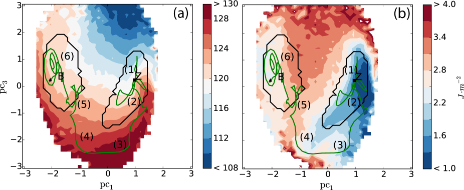
Figure 12: (a) Hemispheric mean kinetic energy $\overline{E}$ in Jm^-2, (b) Hemispheric eddy kinetic energy $E^{\prime}$ in Jm^-2. The green line, starting with a black square and ending with a black triangle, represents a 200 days long trajectory transiting from the zonal to the blocked regime.

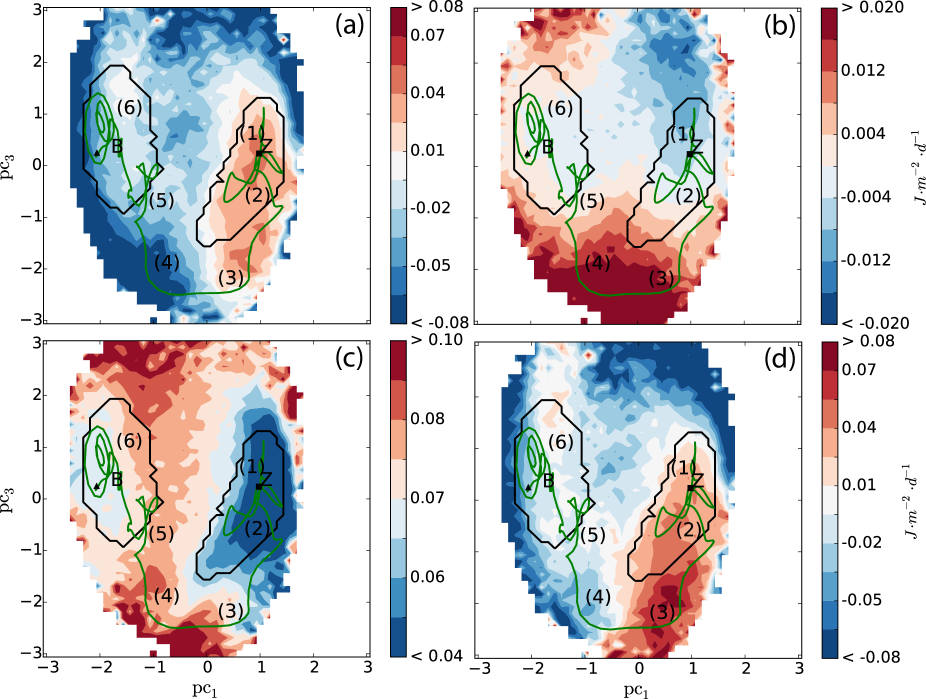
Figure 13: (a) Tendency of the hemispheric mean kinetic energy in Jm^-2day^-1, (b) Tendency of the hemispheric eddy kinetic energy in Jm^-2day^-1, (c) Hemispheric Reynold’s stresses (conversion from mean to eddy kinetic energy when positive) in Jm^-2day^-1, (d) Sum of hemispheric forcing and dissipation in Jm^-2day^-1. The green line, starting with a black square and ending with a black triangle, represents a 200 days long trajectory transiting from the zonal to the blocked regime.

We have seen (section V), that typical trajectories from the zonal to the blocked regime transit through the region of negative $\textnormal{pc}_{3}$. Figures 12 and 13 allow us to give a typical scenario for such a transition. Each step of the following scenario is marked in figures 12 and 13 by the corresponding number.

1. Starting in the zonal regime, the Reynolds’ stress terms are small and the mean flow is stable. However, the positive forcing induces an increase of the mean kinetic energy $\overline{E}$.

2. As $\overline{E}$ increases and the forcing persists, the trajectory evolves to lower value of $\textnormal{pc}_{3}$ and eventually leaves the zonal regime.

3. The trajectory then reaches a region of $\textnormal{pc}_{1}$ close to zero and low $\textnormal{pc}_{3}$. The forcing is still strong but the Reynolds stress terms begin to increase because the strongly sheared flow becomes barotropically unstable for lower values of $\textnormal{pc}_{3}$, so that the total eddy kinetic energy $E^{\prime}$ continues to increase.

4. As the trajectory reaches lower values of $\textnormal{pc}_{1}$, the forcing reverses but the Reynolds’ stress terms continue to increase as the barotropic eddies which emanated at the previous step develop, so that $\overline{E}$ is converted to $E^{\prime}$ which continues to increase.

5. The trajectory then goes to larger values of $\textnormal{pc}_{3}$ where the forcing is negative and energy is removed both from the mean flow and from the eddies so that the barotropic eddies decay.

6. The trajectory eventually reaches the blocked regime for lower values of $\textnormal{pc}_{1}$ where $E^{\prime}$ decreases due to the negative forcing coincident with relatively small Reynolds’ stress terms. The mean flow is once again relatively stable, although not as much as for the zonal regime, as can be seen for the relatively large Reynolds stress terms in the region of largest $\textnormal{pc}_{1}$ inside the blocked regime.

This scenario is consistent with the mechanisms of chaotic itinerancy (Itoh and Kimoto, 1996), heteroclinic connections (Weeks et al., 1997; Crommelin, 2003) and almost-invariant sets bounded by invariant manifolds (Froyland and Padberg, 2009). Indeed, when the reduced state is in the zonal regime, the flow is relatively stable as it belongs to what would be the basin of attraction of the zonal regime. However, as it moves towards the neighborhood of positive forcing, energy is given to the mean flow, the horizontal shear increases and the flow becomes unstable to small perturbations. The increasing Reynolds’ stress term indicates that the perturbation grows, starts to interact with the mean flow and enables the state to leave the basin of attraction of the zonal regime.

VII Summary, Discussion and Conclusions

Using concepts of transfer operators of dissipative dynamical systems, stochastic reduction and meta-stable regimes, we developed an early warning indicator of midlatitude atmospheric regime transitions. It was applied here to the transitions between a zonal and blocked flow in a barotropic hemispheric atmosphere model.

Transfer operators yield the evolution of densities induced by the flow. Markov operators have been estimated on the reduced phase space to approximate the point spectrum of the generator of the transfer operators, namely the Ruelle-Pollicott resonances. Their approximation for different lags have been used to assert the presence of slow dynamics associated with meta-stable regimes and the impact of memory effects on these motions. The presence of rates close to zero and separated from the rest of the spectrum supports the existence of almost-invariant sets associated with meta-stable regimes and with time scales of three to six weeks. Furthermore, the relative constancy of these rates showed that memory effects are weak in the meta-stable regimes and along the transition path from the zonal to the blocked regime.

In order to objectively define these regimes, we have developed an algorithm for the computation of almost-invariant sets based on earlier work in (Dellnitz and Junge, 1999; Froyland and Dellnitz, 2003; Froyland and Padberg, 2009), as well as on optimal Markov chain reduction (Deng et al., 2011; Rosvall and Bergstrom, 2008) and greedy optimization in networks (Clauset et al., 2004). The algorithm attempts to minimize a measure of the distance between the reduced Markov operator (giving the transition probabilities between the almost-invariants) and the original one and allows the detection of sets which are both recurrent and persistent. The algorithm has enabled us to robustly define the blocked and the zonal regimes.

Compared to spectral almost-invariant detection algorithms such as developed earlier by (Dellnitz and Junge, 1997, 1999; Froyland and Dellnitz, 2003; Froyland and Padberg, 2009), which are based on the decomposition of the leading eigenvectors of the transfer operator into characteristic functions supporting the almost-invariant sets, our algorithm is expected to perform better in the detection of more than two almost-invariant sets, since the latter uses an aggregative implementation rather than a divisive one like the spectral algorithms. For example, a similar algorithm (Rosvall and Bergstrom, 2008) has been used for the detection of a dozen of communities, associated with spatial patterns of variability, in a correlation network of sea surface temperature (Tantet and Dijkstra, 2014). In this study, we were only interested in the bi-partition problem and our algorithm showed comparable performance in terms of invariance with respect to that in (Froyland and Padberg, 2009).

The transfer operator based algorithms are also comparable to Hidden Markov Models (HMM, Majda et al., 2006; Franzke et al., 2008), with the difference that the former are non-parametric (no assumption is made on the distribution of the reduced states). Contrary to HMM, our algorithm detects hard clusters (non-overlapping sets) and takes as input the transfer operator rather than directly the time series of the observable. In theory, it would be possible to adapt the algorithm to soft clustering (to allow overlapping between the clusters) but the optimization problem would become harder as it would necessitate another algorithm than the (combinatorial) greedy algorithm.

The energy budget of the model showed that striking similarities exist between regions of low EKE and regions of almost-invariance, weak tendency and small memory effects. Low EKE is indicative of stability of the mean flow and thus of almost-invariance, low tendency as well as weaker memory effects due to the small amplitude of the faster unresolved variables.

The early warning indicator is based on a forecasting scheme involving the evolution of densities by the estimated transfer operator in a two-dimensional reduced phase space spanned by two EOFs of the model. It relies on the Markov approximation of the evolution of an initial density in the neighborhood of the latest observation of the system and on the estimation of the probability to reach the blocked regime. A warning is broadcasted for a lag $\tau_{\mathrm{alarm}}$ if this probability exceeds a prescribed critical probability. The quality of the early warning indicator, as measured by the Peirce Skill Score, is highest for a critical probability of about 0.5 but a smaller critical probability of 0.3 allows to emit warnings two weeks ahead of the event, on average. A next step is to investigate how this promising indicator would perform for more realistic models of atmospheric flow transitions.

While the model here has obvious deficiencies (e.g. the lack of the representation of baroclinic instability), it is one of the midlatitude atmospheric models for which regime transitions are found and hence forms a nice test model for the development of the early warning indicator. The computational procedure can in principle be carried out with a General Circulation Models (GCM) exhibiting regime behavior (Dawson et al., 2012, 2014), if sufficiently long simulations can be performed. Note that in our case, we used a 500,000-day-long simulation ($\sim 1300$ years) to assure the significance of our statistics. However, the dominant part of the spectrum was found to be robust to the use of only $50\times 365$ samples which is the typical size of an operational GCM or a reanalysis record. The question remains if the transfer operator based early warning indicator would perform well with nearly Gaussian GCM or observational data (Dawson et al., 2012, 2014; Majda et al., 2006), where it is not clear whether preferred transition paths between the meta-stable regimes exist.

Another application could be to estimate transfer operators from a long run of an operational weather prediction GCM and use these operators in parallel with a deterministic run of the GCM, in order to account for both uncertainty in the deterministic forecast (Palmer et al., 2005), and to give an early warning indicator of transition to a new meta-stable regime.

Finally, the early warning indicator presented here certainly extends those based on critical slowdown Scheffer et al. (2009), such as the increase in variance and lag-1 autocorrelation, which definitely have problems in high-dimensional phase space. Even the network based indicators (van der Mheen et al., 2013; Viebahn and Dijkstra, 2014; Feng et al., 2014; Tirabassi et al., 2014) are not readily extended to high-dimensional systems. It is therefore hoped that the techniques in this paper will find application in many types of chaotic high-dimensional systems as found in physics and engineering.

Appendix A Bootstrap applied to transition matrices

This appendix is concerned with the limited length of the record used to estimate the transition matrices $\{\hat{P}_{\tau}\}$ defined in section III.2. This statistical inference problem can result in errors, notably in the rates and the regimes calculated from $\{\hat{P}_{\tau}\}$ in section IV.1 and IV.3 respectively, and requires an estimation of confidence intervals.

Following Chekroun et al. (2014), we use a version of the non-parametric bootstrap (Efron, 1980; Mudelsee, 2010), adapted to the estimation of transition matrices as done in (Craig and Sendi, 2002). It starts from the matrix $T_{\tau}$ counting the transitions of $\{y_{t}\}$ from one grid box to another, before the normalization has been applied to get the transition probabilities. From $T_{\tau}$, $N_{s}$ surrogate count matrices $\{T_{\tau,s}^{*}\}_{1\leq s\leq N_{s}}$ are generated. This is done, for each row $i$, by taking with replacement $n_{i}$ target grid boxes among the $n_{i}$ transitions starting from grid-box $B_{i}$ of $T_{\tau}$. This accounts for drawing $n_{i}$ times from a Multinomial distribution with vector of probabilities $\{(\hat{P}_{\tau})_{il}\}_{1\leq l\leq m}$. From these $N_{s}$ surrogate count matrices, the transition matrices $\{\hat{P}_{\tau,s}^{*}\}_{1\leq s\leq N_{s}}$ are then calculated by normalizing their rows. These matrices can then be used to estimate the sampling error of any functions of the transition matrix $\hat{P}_{\tau}$.

A thousand surrogate matrices $\{\hat{P}_{\tau,s}^{*}\}_{1\leq s\leq N_{s}}$ are used to compute $99\%$ confidence intervals for the rates represented in figure 4. For each lag $\tau$, the leading rates have been calculated for every surrogate transition matrix in $\{\hat{P}_{\tau,s}^{*}\}_{1\leq s\leq N_{s}}$. For each rate $r_{i}(\tau)$ one gets a distribution of surrogate rates $\{(r_{i}(\tau))_{s}^{*}\}_{1\leq s\leq N_{s}}$. After sorting these distributions, the $(0.005*N_{s})^{th}$ and the $(0.995*N_{s})^{th}$ values are taken to give the lower bound and the upper bound, respectively, of the confidence interval for rate $r_{i}(\tau)$.

In this study, we added a bias correction to the intervals because the described construction of the surrogate matrices introduces a bias towards lower values for rates, in particular for the secondary rates. We give an example to explain this bias. Assume that only two transitions start from a box $B_{i}$, with targets $B_{k}$ and $B_{l}$. In the surrogate, the probability to pick two different transitions ($B_{k}$ and $B_{l}$) will be of $1/2$, while the probability to pick two of the same transitions (twice $B_{k}$ or twice $B_{l}$) will also be of $1/2$. Thus, a bias is introduced towards a weaker mixing resulting in lower values of the rates (in particular to the secondary ones more sensitive to such details). This bias was removed by centering the mean of the surrogate rates $\{(r_{i}(\tau))_{s}^{*}\}_{1\leq s\leq N_{s}}$ to the the value of the original rate $r_{i}(\tau)$ being tested.

The surrogate transition matrices $\{\hat{P}_{\tau,s}^{*}\}_{1\leq s\leq N_{s}}$ can also be used to test the robustness of the regimes to the sampling by running, for each $\hat{P}_{\tau,s}^{*}$, the regime detection algorithm described in section IV.3. The membership of a grid box to a regime can be given by a membership matrix $M_{i\beta}$ such that $M_{i\beta}=1$ if grid box $B_{i}$ belongs to regime $E_{\beta}$, and is zero otherwise. Confidence intervals are not well suited for statistics taking logical values. Instead, we compute, for each grid-box $B_{i}$, the fraction of surrogates for which $B_{i}$ belongs to regime $E_{\beta}$. These fractions are plotted in figure 14a,b for the blocked and the zonal regime, respectively, using $N_{s}=100$ surrogates.

We can see that the core of the regimes are very robust to the sampling, as indicated by the amount of grid boxes in each regime for which a fraction close to a $100\%$ of the boxes of the surrogates have been attributed to the same regime. However, boxes along the path of the transition from the zonal to the blocking regimes are less robust to the sampling. Such exit-region and entering-region for the zonal and the blocked regime, respectively, are indeed harder to attribute to a regime, since they correspond to regions where the invariance is weak. A possibility would be to add a simulated annealing step in the almost-invariant sets detection algorithm as has been used, for example, in Rosvall and Bergstrom (2008).

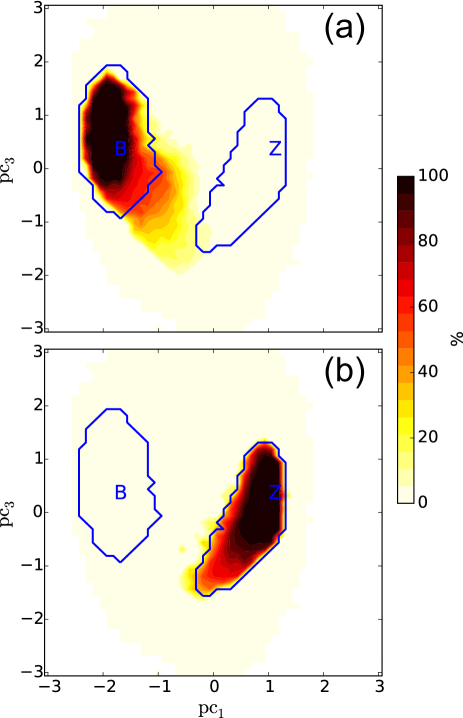
Figure 14: The value at each grid box represents the fraction of surrogate regimes for which the grid box belongs to (a) the blocked regime or (b) the zonal regime out of a $100$ surrogates. The surrogate regimes were detected by applying the algorithm of section IV.3 to the bootstrap surrogate transition matrices.

Appendix B Robustness to grid resolution

The robustness of the rates and the regimes to the grid resolution for which the transition matrices are estimated is tested next.

Figure 15a, b represent rates calculated from transition matrices estimated on a grid of $10\times 10$ and $100\times 100$ boxes respectively, to be compared with figure 4 of section IV.1. We can see that at least the $3$ leading rates in green, red and cyan are not much affected by the grid resolution so that the analysis of section IV.1 remains valid under changes of the grid in this range. This robustness to the grid of the leading rates is in agreement with the fact that they represent slow large-scale motions less likely to be affected by small perturbations of the transition matrices.

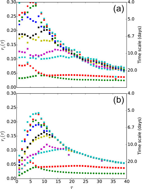
Figure 15: Rates $r_{i}(\tau)$ as in figure 4 but calculated from estimates of transition matrices on a (a) $10\times 10$ grid and (b) $100\times 100$ grid.

Figure 16a,b represent regimes detected from transition matrices estimated on a grid of $20\times 20$ and $200\times 200$ boxes respectively, to be compared with figure 6 of section IV.3. It can be seen that in both cases the regimes are very much alike to the one plotted figure 6 for the grid of $50\times 50$ boxes. The quality of the regimes deteriorates for grids coarser than $20\times 20$ (not represented here) but remains relatively good for resolutions as refined as $200\times 200$ (Fig. 16.b). This robustness of the regimes to very refined resolutions can be explained by the aggregative nature of the almost-invariant sets detection algorithm. Indeed, one expects the estimates of the transition probabilities between grid boxes to deteriorate as the grid becomes thinner and as the number of samples by grid box decreases. However, because the algorithm iteratively agglomerates grid boxes into clusters, the transition probabilities between these coarser and coarser clusters become less and less sensitive to the sampling as the number of samples by clusters increases with their size.

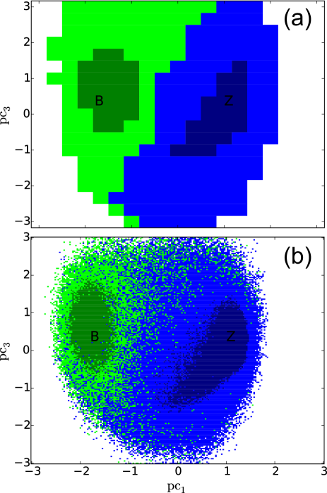
Figure 16: Almost-invariant sets and their regimes as for figure 6 but for a grid of (a) $20\times 20$ and (b) $200\times 200$.

Appendix C Robustness of the regimes to the time lag

In addition to the robustness test of the regimes to the grid resolution, we next test their robustness to the choice of the time lag of the transition matrix from which they are detected. Regimes detected for lags $\tau$ of 7 and 50 days are plotted in figure 17a,b, respectively, to be compared to figure 6 of section IV.3. In this range, we can see that the quality of the regimes is robust to the lag.

For lags shorter than 7 days, however, the algorithm is not able to distinguish the transition path between the zonal and the blocked regime from the regimes themselves (not shown here). Such result is in agreement with the fact that for lags smaller than $7$ days, the complex pair of rates represented by green squares in figure 4, more likely to be associated with the transition, is dominant over the real eigenvalue represented by red circles and likely to be associated with the meta-stability of the regimes. Thus the motions associated with the transition appear to be dominant over the meta-stability of the regimes for such short lags.

The deterioration of the regimes for lags larger that $50$ days is to be expected due to the fact that, as seen section IV.1, the leading rates of figure 4, associated with meta-stability, have time-scales not larger than $40$ days, so that for longer lags, the motions associated with the meta-stable regimes are likely to decorrelate and cannot be detected by the algorithm.

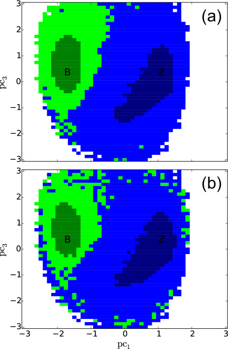
Figure 17: Almost-invariant sets and their regimes as for figure 6 but for a lag of (a) 7 days and (b) 50 days.

Appendix D Test of the semigroup property

In this appendix, we justify that the distances plotted in figure 5a in section IV.1, between densities transferred by a power of 2 of $\hat{P}_{8}$ and densities transferred by $\hat{P}_{2\times 8}$, are mostly explained by memory effects rather than by the Galerkin approximation or by the sampling.

To do so, we first represent the same distances but calculated from transition matrices estimated from time series of only $250,000$ realizations and as much as $1,000,000$ realizations (Fig. 18.a and b respectively), compared to the $500,000$ realizations from which the distances represented figure 5 have been calculated. We can see that neither plots seem to be affected by the short or long length of the time-series. One has to go to record lengths shorter than $200,000$ realizations to start to see a difference in the distances (not shown here). Thus, the distances represented in figure 5 are not likely to be due to the limited length of the time-series from which the transition probabilities have been calculated.

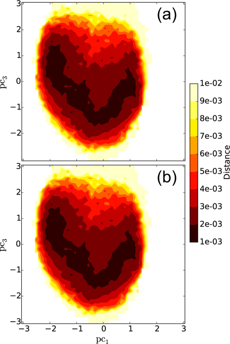
Figure 18: As for figure 5, the value at each grid-point represents the distance, for an initial density of 1 at this grid-point, between the density $f_{8k}^{\mathrm{pow}}$ transferred by the $k^{th}$ poser of $\hat{P_{8}}$ and a density $f_{8k}^{\mathrm{long}}$ transferred by $\hat{P}_{k\times 8}$ for $k=2$. However, the transition matrices have been estimated from a time series of (a) $250,000$ days and (b) $1,000,000$ days, compared to the $500,000$ of figure 5.

Secondly, to test the effect of the Galerkin approximation on the distances, we have again reproduced figure 5, using $500,000$ realizations, but with a grid of $20\times 20$ and $100\times 100$ (Fig. 19.a and b respectively). While for the $20\times 20$ grid, the distances get larger, indicating that this increase is due to the Galerking approximation, the distances for the $100\times 100$ grid resolution (Fig. 19.b) are very much alike the one for the $50\times 50$ resolution (Fig. 5). Note that this is also true when a record length of $1,000,000$ realizations (not shown here), so that the similarities between the plots is not likely to be due to a compensating effect between the grid resolution and the number of samples per grid point.

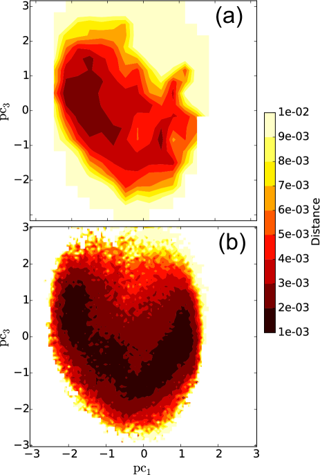
Figure 19: As for figure 5, the value at each grid-point represents the distance, for an initial density of 1 at this grid-point, between the density $f_{8k}^{\mathrm{pow}}$ transferred by the $k^{th}$ poser of $\hat{P_{8}}$ and a density $f_{8k}^{\mathrm{long}}$ transferred by $\hat{P}_{k\times 8}$ for $k=2$. However, the transition matrices have been estimated from on a grid of (a) $20\times 20$ and (b) $100\times 100$ boxes, compared to the $50\times 50$ boxes of figure 5.

We can thus conclude that the distances represented in figure 5 for $\hat{P}_{8}^{2}$ and $\hat{P}_{2\times 8}$ are mostly due to memory effects introduced by the only partial observation of the barotropic model.

References

References

- Lorenz (1963) E. Lorenz, Journal of the atmospheric sciences 20, 130 (1963).
- Palmer (1993) T. N. Palmer, Weather 48, 314 (1993).
- James (1994) I. N. James, Introduction to Circulating Atmospheres, edited by R. W. Houghton, M. J. Rycroft, and A. J. Dessler (Cambridge University Press, Cambridge, 1994).
- Mo et al. (1988) K. C. Mo, M. Ghil, P. Physics, and L. Angeles, Journal of Geophysical Research 93, 10927 (1988).
- Kimoto and Ghil (1993) M. Kimoto and M. Ghil, Journal of the atmospheric sciences 50, 2625 (1993).
- Smyth et al. (1999) P. Smyth, K. Ide, M. Ghil, C. Science, P. Physics, and L. Angeles, Journal of the atmospheric sciences 56, 3704 (1999).
- Plaut and Vautard (1994) G. Plaut and R. Vautard, Journal of the atmospheric sciences 51, 210 (1994).
- Ghil and Robertson (2002) M. Ghil and A. Robertson, Proceedings of the National Academy of Sciences of the United States of America 99, 2493 (2002).
- Kondrashov et al. (2004) D. Kondrashov, K. Ide, and M. Ghil, Journal of the atmospheric sciences 61, 568 (2004).
- Smyth (1999) P. Smyth, Statistics and Computing 3425, 63 (1999).
- Majda et al. (2006) A. J. Majda, C. L. Franzke, A. Fischer, and D. Crommelin, Proceedings of the National Academy of Sciences of the United States of America 103, 8309 (2006).
- Franzke et al. (2008) C. L. Franzke, D. Crommelin, A. Fischer, and A. J. Majda, Journal of Climate 21, 1740 (2008).
- Stephenson et al. (2004) D. B. Stephenson, a. Hannachi, and a. O’Neill, Quarterly Journal of the Royal Meteorological Society 130, 583 (2004).
- Christiansen (2007) B. Christiansen, Journal of Climate 20, 2229 (2007).
- Fereday et al. (2008) D. R. Fereday, J. R. Knight, A. A. Scaife, C. K. Folland, and A. Philipp, Journal of Climate 21, 3687 (2008).
- Dawson et al. (2012) A. Dawson, T. N. Palmer, and S. Corti, Geophysical Research Letters 39, L21805 (2012).
- Jung et al. (2005) T. Jung, T. N. Palmer, and G. J. Shutts, Geophysical Research Letters 32, L23811 (2005).
- Dawson et al. (2014) A. Dawson, T. N. Palmer, and S. Corti, Climate Dynamics (2014), 10.1029/2012GL053284.
- Charney and DeVore (1979) J. G. Charney and J. G. DeVore, Journal of the atmospheric sciences 36, 1205 (1979).
- Weeks et al. (1997) E. R. Weeks, H. L. Swinney, and M. Ghil, Science 278, 1598 (1997).
- Williams (2003) P. D. Williams, Geophysical Research Letters 30, 2255 (2003).
- Williams et al. (2004) P. D. Williams, T. W. N. Haine, and P. L. Read, Nonlinear Processes in Geophysics 11, 127 (2004).
- Williams et al. (2005) P. D. Williams, T. W. N. Haine, and P. L. Read, Journal of Fluid Mechanics 528, 1 (2005).
- Williams et al. (2008) P. D. Williams, T. W. N. Haine, and P. L. Read, Journal of the atmospheric sciences 65, 3543 (2008).
- Kaneko (1991) K. Kaneko, Physica D: Nonlinear Phenomena 54, 5 (1991).
- Itoh and Kimoto (1996) H. Itoh and M. Kimoto, Journal of the atmospheric sciences 53, 2217 (1996).
- Crommelin et al. (2004) D. Crommelin, J. D. Opsteegh, F. Verhulst, and D. Bilt, Journal of the atmospheric sciences 61, 1406 (2004).
- Crommelin (2003) D. Crommelin, Journal of the atmospheric sciences 60, 229 (2003).
- Selten (1995) F. M. Selten, Journal of the atmospheric sciences 52, 915 (1995).
- Legras and Ghil (1985) B. Legras and M. Ghil, Journal of the atmospheric sciences 42, 433 (1985).
- Branstator and Opsteegh (1989) G. Branstator and J. D. Opsteegh, Journal of the atmospheric sciences 46, 1799 (1989).
- Gardiner (2009) C. W. Gardiner, Handbook of Stochastic Methods, edited by H. Haken (Springer, Berlin Heidelberg, 2009) p. 447.
- Penland (2003) C. Penland, Bulletin of the American Meteorological Society 84, 921 (2003).
- Majda et al. (1999) A. J. Majda, I. Timofeyev, and E. Vanden-Eijnden, Proceedings of the National Academy of Sciences 96, 14687 (1999).
- Majda et al. (2001) A. J. Majda, I. Timofeyev, and E. Vanden-Eijnden, Communications on Pure and Applied Mathematics 54, 891 (2001).
- Franzke et al. (2005) C. L. Franzke, A. J. Majda, and E. Vanden-Eijnden, Journal of the atmospheric sciences 62, 1722 (2005).
- Franzke et al. (2015) C. L. Franzke, T. J. O’Kane, J. Berner, P. D. Williams, and V. Lucarini, Wiley Interdisciplinary Reviews: Climate Change 6, 63 (2015).
- Chorin and Hald (2009) A. J. Chorin and O. H. Hald, Stochastic tools in mathematics and science, edited by S. Antman, P. Holmes, and K. Sreenivasan (Springer, New York Heidelberg Dordrecht London, 2009).
- Darve et al. (2009) E. Darve, J. Solomon, and A. Kia, Proceedings of the National Academy of Sciences of the United States of America 106, 10884 (2009).
- Wouters and Lucarini (2013) J. Wouters and V. Lucarini, Journal of Statistical Physics 151, 850 (2013), arXiv:arXiv:1208.3080v2 .
- Kondrashov et al. (2015) D. Kondrashov, M. D. Chekroun, and M. Ghil, Physica D 297, 33 (2015).
- Palmer and Williams (2009) T. N. Palmer and P. D. Williams, Stochastic Physics and Climate Modelling, edited by P. Williams and T. Palmer (Cambridge University Press, Cambridge, 2009) p. 496.
- Lasota and Mackey (1994) A. Lasota and M. C. Mackey, Chaos, Fractals and Noise, edited by J. E. Marsden and L. Sirovich (Springer, Berlin, 1994).
- Froyland and Padberg-gehle (2014) G. Froyland and K. Padberg-gehle, Ergodic Theory, Open Dynamics, and Coherent Structures, edited by W. Bahsoun, C. Bose, and G. Froyland, Springer Proceedings in Mathematics & Statistics, Vol. 70 (Springer New York, New York, NY, 2014) pp. 171–216.
- Pollicott (1985) M. Pollicott, Inventiones Mathematicae 81, 413 (1985).
- Ruelle (1986a) D. Ruelle, Physical review letters 56, 405 (1986a).
- Ruelle (1986b) D. Ruelle, Journal of statistical physics 44, 281 (1986b).
- Butterley and Liverani (2007) O. Butterley and C. Liverani, Journal of Modern Dynamics 1, 301 (2007).
- Chekroun et al. (2014) M. D. Chekroun, J. D. Neelin, D. Kondrashov, J. C. McWilliams, and M. Ghil, Proceedings of the National Academy of Sciences of the United States of America 111, 1684 (2014).
- Scheffer et al. (2009) M. Scheffer, J. Bascompte, W. a. Brock, V. Brovkin, S. R. Carpenter, V. Dakos, H. Held, E. H. van Nes, M. Rietkerk, and G. Sugihara, Nature 461, 53 (2009).
- van der Mheen et al. (2013) M. van der Mheen, H. a. Dijkstra, A. Gozolchiani, M. den Toom, Q. Feng, J. Kurths, and E. Hernandez-Garcia, Geophysical Research Letters 40, 2714 (2013).
- Viebahn and Dijkstra (2014) J. Viebahn and H. a. Dijkstra, International Journal of Bifurcation and Chaos 24, 1430007 (2014).
- Feng et al. (2014) Q. Y. Feng, J. P. Viebahn, and H. a. Dijkstra, Geophysical Research Letters 41, 6008 (2014).
- Tirabassi et al. (2014) G. Tirabassi, J. Viebahn, V. Dakos, H. a. Dijkstra, C. Masoller, M. Rietkerk, and S. Dekker, Ecological Complexity 19, 148 (2014).
- Peirce (1884) C. S. Peirce, Science 4, 453 (1884).
- Stephenson (2000) D. B. Stephenson, Weather and Forecasting 15, 221 (2000).
- Thornes and Stephenson (2001) J. E. Thornes and D. B. Stephenson, Meteorological Applications 8, 307 (2001).
- Roads (1987) J. Roads, Journal of the atmospheric sciences 44, 3495 (1987).
- von Storch and Zwiers (1999) H. von Storch and F. W. Zwiers, in Statistical Analysis in Climate Research (Cambridge University Press, Cambridge, 1999) Chap. 13, pp. 293–316.
- Givon et al. (2004) D. Givon, R. Kupferman, and A. Stuart, Nonlinearity 17, R55 (2004).
- Rudin (1991) W. Rudin, Functional Analysis, edited by L. Gurley, R. Wallis, and M. Luhrs (McGraw-Hill, New York, 1991) p. 424.
- Gouëzel and Liverani (2006) S. Gouëzel and C. Liverani, Ergodic Theory and Dynamical Systems 26, 189 (2006).
- Eckmann and Ruelle (1985) J.-P. Eckmann and D. Ruelle, Reviews of modern physics 57, 617 (1985).
- Young (2002) L.-S. Young, Journal of Statistical Physics 108, 733 (2002).
- Engel and Nagel (2001) K.-J. Engel and R. Nagel, One-parameter semigroups for linear evolution equations, edited by S. Axler, F. W. Gehring, and K. A. Ribet (Springer, New York Berlin Heidelberg Barcelona Hong Kong London Milan Paris Singapore Tokyo, 2001) p. 586.
- Gallavotti and Cohen (1995) G. Gallavotti and E. G. D. Cohen, Journal of Statistical Physics 80, 931 (1995).
- Kifer (1986) Y. Kifer, Journal d’Analyse Mathématique 47, 111 (1986).
- Dellnitz and Junge (1999) M. Dellnitz and O. Junge, SIAM Journal on Numerical Analysis 36, 491 (1999).
- Blank et al. (2002) M. Blank, G. Keller, and C. Liverani, Nonlinearity 15, 1905 (2002).
- Keller et al. (1998) G. Keller, C. Liverani, and T. U. D. Roma, Stability of the spectrum for transfer operators, Tech. Rep. (ANN. SCUOLA NORM. SUP. PISA CL SCI, 1998).
- Baladi and Holschneider (1999) V. Baladi and M. Holschneider, Nonlinearity 12, 525 (1999).
- Froyland (2001) G. Froyland, in Nonlinear dynamics and statistics, edited by A. I. Mees (Birkhäuser Boston, Boston, 2001) Chap. 12, pp. 281–321.
- Ulam (1964) S. M. Ulam, “Problems in Modern Mathematics,” (1964).
- Froyland (1998) G. Froyland, Nonlinear Analysis: Theory, Methods & Applications 32, 831 (1998).
- Billingsley (1961) P. Billingsley, Statistical Inference for Markov process (University of Chicago Press, Chicago, 1961).
- Froyland et al. (2013) G. Froyland, O. Junge, and P. Koltai, SIAM Journal on Numerical Analysis 51, 223 (2013).
- Baladi (2000) V. Baladi, Positive Transfer Operators and Decay of Correlations, edited by R. S. MacKay (World Scientific, Singapore, 2000) p. 314.
- Froyland and Padberg (2009) G. Froyland and K. Padberg, Physica D: Nonlinear Phenomena 238, 1507 (2009).
- Dellnitz and Junge (1997) M. Dellnitz and O. Junge, International Journal of Bifurcation and Chaos 7, 2475 (1997).
- Froyland and Dellnitz (2003) G. Froyland and M. Dellnitz, SIAM Journal on Scientific Computing 24, 1839 (2003).
- DelSole (2000) T. DelSole, Journal of the atmospheric sciences 57, 2158 (2000).
- Berner (2005) J. Berner, Journal of the atmospheric sciences 62, 2098 (2005).
- Crommelin and Vanden-Eijnden (2011) D. Crommelin and E. Vanden-Eijnden, Multiscale Modeling & Simulation 9, 1588 (2011).
- Penland and Sardeshmukh (1995) C. Penland and P. Sardeshmukh, Journal of climate 8, 1999 (1995).
- Deng et al. (2011) K. Deng, P. Mehta, and S. Meyn, Automatic Control, IEEE 56, 2793 (2011).
- Rosvall and Bergstrom (2008) M. Rosvall and C. T. Bergstrom, Proceedings of the National Academy of Sciences of the United States of America 105, 1118 (2008).
- Cover and Thomas (1991) T. M. Cover and J. A. Thomas, in Elements of Information Theory (John Wiley & Sons, New Jersey, 1991) Chap. 2, pp. 13–55.
- Clauset et al. (2004) A. Clauset, M. Newman, and C. Moore, Physical Review E 70, 066111 (2004).
- Kharin and Zwiers (2003) V. Kharin and F. Zwiers, Journal of Climate 16, 4145 (2003).
- Branstator and Berner (2005) G. Branstator and J. Berner, Journal of the atmospheric sciences 62, 1792 (2005).
- Tantet and Dijkstra (2014) A. Tantet and H. a. Dijkstra, Earth System Dynamics 5, 1 (2014).
- Palmer et al. (2005) T. N. Palmer, G. Shutts, R. Hagedorn, F. Doblas-Reyes, T. Jung, and M. Leutbecher, Annual Review of Earth and Planetary Sciences 33, 163 (2005).
- Efron (1980) B. Efron, The Jacknife, the bootstrap, and other resampling plans, Tech. Rep. (Stanford University, Stanford, 1980).
- Mudelsee (2010) M. Mudelsee, Climate Time Series Analysis: Classical Statistical and Bootstrap Methods, edited by L. A. Mysak and K. Hamilton (Springer, Dordrecht Heidelberg London New York, 2010) p. 474.
- Craig and Sendi (2002) B. a. Craig and P. P. Sendi, Health economics 11, 33 (2002).