Finite Temperature Quantum Effects in Many-body Systems by Classical Methods

Abstract

A recent description of an exact map for the equilibrium structure and thermodynamics of a quantum system onto a corresponding classical system is summarized. Approximate implementations are constructed by pinning exact limits (ideal gas, weak coupling), and illustrated by calculation of pair correlations for the uniform electron gas and shell structure for harmonically confined charges. A wide range of temperatures and densities are addressed in each case. For the electron gas, comparisons are made to recent path integral Monte Carlo simulations (PIMC) showing good agreement. Finally, the relevance for orbital free density functional theory for conditions of warm, dense matter is discussed briefly.

Keywords: quantum many-body, classical map, electron gas, charges in trap, density functional theory

1 Introduction and Motivation

A fundamental description of the thermodynamics (e.g., free energy) and structure (e.g., pair correlation function) for materials comprised of electrons and ions remains a challenge for many state conditions of current interest [1]. Typically the ions can be described by semi-classical methods due to their relatively large masses. In contrast, the electrons may require an accurate description of strong quantum effects. Typical solid state conditions occur at temperatures well below the electron Fermi temperature for which the multiplicity of zero temperature many-body theories and simulations are available. However, as the temperature is increased to several times the Fermi temperature such methods fail or become increasingly difficult to implement. At still higher temperatures, effective classical methods can be applied (e.g., molecular dynamics simulation [2], Monte Carlo integration, classical density functional theory [3], liquid state theory [4]). There is a long history of phenomenological attempts to extend these classical methods to lower temperature by including quantum effects in modified pair potentials [5]. More recently, these effective classical systems have been improved significantly by the inclusion of quantum effects in a modified classical temperature [6, 7, 8]. The entire approach of constructing a classical system to replicate the thermodynamics and structure has been given a formally exact context from which more controlled approximations can be constructed [9, 10]. The objective here is to summarize briefly this latter work and to illustrate its utility by two applications: 1) the calculation of pair correlations for the uniform electron gas, and 2) the description of shell structure for charges in a harmonic trap. In both cases the emphasis is on conditions ranging from classical to strongly quantum mechanical. The last section describes how this effective classical approach can be exploited to address current problems of ”warm, dense matter” via orbital free density functional theory [1].

2 Definition of the Effective Classical System

Consider a system of $N$ particles in a volume $V$ with pairwise interactions and an external single particle potential. The Hamiltonian is

$$H_{N}=K+\Phi+\sum_{i}^{N}v\left(\mathbf{q}_{i}\right),$$ (1)

where $K$ and $\Phi$ are the total kinetic and potential energies, respectively. The form of the pair potential $\phi\left(\mathbf{q}_{i},\mathbf{q}_{j}\right)$ and external potential $v\left(\mathbf{q}_{i}\right)$ is left general at this point. The equilibrium thermodynamics for this system in the Grand Canonical ensemble is determined from the grand  potential $\Omega(\beta\mid\mu,\phi)$

$$\beta\Omega(\beta\mid\mu,\phi)=-\ln\sum_{N}Tr_{N}e^{-\beta\left(K+\Phi-\int d\mathbf{r}\mu(\mathbf{r})\widehat{n}(\mathbf{r})\right)}.$$ (2)

Here the local chemical potential $\mu(\mathbf{r})$ is defined by

$$\mu(\mathbf{r})=\mu-v(\mathbf{r}),$$ (3)

and the operator $\widehat{n}(\mathbf{r})$ representing the microscopic density is defined by

$$\widehat{n}(\mathbf{r})=\sum_{i=1}^{N}\delta\left(\mathbf{r}-\mathbf{q}_{i}\right).$$ (4)

The notation $\Omega(\beta\mid\mu,\phi)$ indicates that it is a function of the inverse temperature $\beta^{-1}=k_{B}T$ and a functional of $\mu(\mathbf{r})$ and the pair potential $\phi\left(\mathbf{r},\mathbf{r}^{\prime}\right)$.

A corresponding classical system is defined with a classical grand potential

$$\beta\Omega_{c}(\beta_{c}\mid\mu_{c},\phi_{c})=-\ln\sum_{N}\frac{1}{\lambda_{c}^{3N}N!}\int d\mathbf{q}_{1}..d\mathbf{q}_{N}e^{-\beta_{c}\left(\Phi_{c}-\int dr\mu_{c}(r)\widehat{n}(r)\right)},$$ (5)

where $\lambda_{c}=\left(2\pi\beta_{c}\hbar^{2}/m\right)^{1/2}$ is the thermal de Broglie wavelength and the inverse temperature of the quantum system $\beta$ multiplies the classical grand potential. The classical grand potential is defined in terms of an effective inverse classical temperature $\beta_{c}$, effective classical local chemical potential $\mu_{c}(\mathbf{r})$, and effective classical pair potential $\phi_{c}\left(\mathbf{r},\mathbf{r}^{\prime}\right).$ The classical system therefore has one undetermined scalar and two undetermined functions. These are defined by the following three conditions

$$\Omega_{c}(\beta_{c}\mid\mu_{c},\phi_{c})\equiv\Omega(\beta\mid\mu,\phi),\hskip 18.06749pt\frac{\delta\Omega_{c}(\beta_{c}\mid\mu_{c},\phi_{c})}{\delta\mu_{c}(\mathbf{r})}\mid_{\beta_{c},\phi_{c}}\equiv\frac{\delta\Omega(\beta\mid\mu,\phi)}{\delta\mu(\mathbf{r})}\mid_{\beta},$$ (6)

$$\frac{\delta\Omega_{c}(\beta_{c}\mid\mu_{c},\phi_{c})}{\delta\phi_{c}(\mathbf{r},\mathbf{r}^{\prime})}\mid_{\beta_{c},\mu_{c}}=\frac{\delta\Omega(\beta\mid\mu,\phi)}{\delta\phi(\mathbf{r},\mathbf{r}^{\prime})}\mid_{\beta,\mu}.$$ (7)

An equivalent form for these conditions can be expressed in terms of the pressure, the local average density, and the pair correlation function

$$p_{c}(\beta_{c}\mid\mu_{c},\phi_{c})\equiv p(\beta\mid\mu,\phi),\hskip 18.06749ptn_{c}(\mathbf{r;}\beta_{c}\mid\mu_{c},\phi_{c})\equiv n(\mathbf{r;}\beta\mid\mu,\phi),$$ (8)

$$g_{c}(\mathbf{r},\mathbf{r}^{\prime};\beta_{c}\mid\mu_{c},\phi_{c})\equiv g(\mathbf{r},\mathbf{r}^{\prime};\beta\mid\mu,\phi).$$ (9)

In this way the classical system has the same thermodynamics and structure as that of the underlying quantum system.

These definitions for $\beta_{c},\mu_{c},$ and $\phi_{c}$ are only implicit and require inversion of the classical expressions on the left sides of these equations to express them in terms of the given quantum variables $\beta,\mu,$ and $\phi.$ Generally this is a difficult classical many-body problem. In addition, the inversion is expressed in terms of the corresponding quantum functions $p(\beta\mid\mu,\phi)$, $n(\mathbf{r;}\beta\mid\mu,\phi),$ and $g(\mathbf{r},\mathbf{r}^{\prime};\beta\mid\mu,\phi)$ which require solution to the original difficult quantum many-body problem. Hence it would appear that the introduction of a representative classical system to calculate the thermodynamics of the quantum system is circular. However, it is expected that the inversion can be accomplished in some simple approximation that incorporates relevant quantum effects and the resulting approximate classical parameters $\beta_{c},\mu_{c},$ and $\phi_{c}$ used in a more accurate theory or simulation to ”bootstrap” a better thermodynamics and structure. This is illustrated in the next two sections.

3 Pair Correlations in the Uniform Electron Gas

To illustrate the utility and effectiveness the effective classical system approach defined above, the calculation of pair correlations in the uniform electron gas is described in this section. The objective is to describe these correlations over the entire density and temperature plane. In the classical domain this system is typically known as the one component plasma. The classical system is well-described by classical methods such as liquid state theory, classical Monte Carlo, and molecular dynamics simulation. Both fluid and solid equilibrium phases are now well characterized, including very strong coupling conditions. Consequently, there is a great potential to apply these approaches as well to quantum systems using the classical map.

In this section the system of interest is the uniform electron gas at equilibrium. It is comprised of electrons in a uniform neutralizing background. The dimensionless temperature used here is the temperature relative to the Fermi temperature, $t\equiv 1/\beta\epsilon_{F}$, where the Fermi energy is defined by $\epsilon_{F}=\hbar^{2}\left(3\pi^{2}n\right)^{2/3}/2m$ . Also the density dependence is characterized by the ratio of the average distance between particles relative to the Bohr radius, $r_{s}\equiv r_{0}/a_{B}$, where $4\pi nr_{0}^{3}/3=1$ and $a_{B}=\hbar^{2}/me^{2}$. The dimensionless space scale is $\mathbf{r}^{\ast}\mathbf{=r}/r_{0}$. The classical pair correlation function at uniform equilibrium depends only on the relative coordinate so

$$g_{c}(\mathbf{r},\mathbf{r}^{\prime};\beta_{c}\mid\mu_{c},\phi_{c})\equiv g_{c}(\left|\mathbf{r}^{\ast}-\mathbf{r}^{\ast\prime}\right|,r_{s}\mid\phi_{c}^{\ast}),$$ (10)

where $\phi_{c}^{\ast}\equiv\beta\phi^{\ast}=\Gamma/\left|\mathbf{r}^{\ast}-\mathbf{r}^{\ast\prime}\right|$. Here $\Gamma=\beta e^{2}/r_{0}$ is the classical Coulomb coupling constant. In terms of $t,r_{s}$ it is $\Gamma=2\left(\frac{9}{4}\pi\right)^{-2/3}r_{s}t^{-1}$. Note that the functional $g_{c}(r,r_{s}\mid\cdot)$ is independent of $t$. In contrast, the quantum pair correlation functional depends on both $r_{s}$ and $t$

$$g(\mathbf{r},\mathbf{r}^{\prime};\beta\mid\mu_{c},\phi_{c})\equiv g(\left|\mathbf{r}^{\ast}-\mathbf{r}^{\ast\prime}\right|,r_{s},t\mid\phi^{\ast}).$$ (11)

Now, using the equivalence of the classical and quantum pair correlation functions (9) the classical functional can be inverted to give $\phi_{c}^{\ast}$

$$\phi_{c}^{\ast}\left(r^{\ast},r_{s},t\right)=g_{c}^{-1}(r^{\ast},r_{s}\mid g).$$ (12)

This is the formally exact definition of the effective classical pair potential. The practical procedure is to evaluate this in some reasonable, simple approximation and then ”bootstrap” the result in a more sophisticated approximation to $g_{c}(r^{\ast},r_{s}\mid\phi_{c}^{\ast}).$ First, it is required that the limit of non-interacting particles be given correctly, so the potential is written as

$$\phi_{c}^{\ast}\left(r^{\ast},r_{s},t\right)=\phi_{c}^{\ast(0)}\left(r^{\ast},r_{s},t\right)+\Delta\left(r^{\ast},r_{s},t\right).$$ (13)

Here $\phi_{c}^{\ast(0)}\left(r^{\ast},r_{s},t\right)$ is an effective pair interaction chosen such that its classical pair correlation function is the same as that for the quantum system with no Coulomb interactions, $g^{(0)}\left(r^{\ast},r_{s},t\right).$ The second term, $\Delta\left(r^{\ast},r_{s},t\right)$, replaces the Coulomb interaction by a corresponding classical pair interaction incorporating the quantum effects. Here, it is constrained to be exact in the weak coupling limit. Classically, the latter corresponds to the potential becoming the same as the direct correlation function

$$\phi_{c}^{\ast}\left(r^{\ast},r_{s},t\right)\rightarrow-c\left(r^{\ast},r_{s},t\right),\hskip 18.06749pt\phi_{c}^{\ast(0)}\left(r^{\ast},r_{s},t\right)\rightarrow-c^{(0)}\left(r^{\ast},r_{s},t\right)$$ (14)

where the direct correlation function is defined by the Ornstein-Zernicke equation

$$c\left(r^{\ast},r_{s},t\right)=g\left(r^{\ast},r_{s},t\right)-1-\frac{3}{4\pi}\int d\mathbf{r}^{\prime}c\left(r^{\ast\prime},r_{s},t\right)\left(g\left(\left|\mathbf{r}^{\ast}-\mathbf{r}^{\ast\prime}\right|,r_{s},t\right)-1\right).$$ (15)

The quantum weak coupling limit is the random phase approximation. Therefore (15) is calculated by inserting the finite temperature random phase approximation, $g^{RPA}\left(r^{\ast},r_{s},t\right),$ on the right side. The resulting approximate effective pair potential is now (13) with

$$\phi_{c}^{\ast}\left(r^{\ast},r_{s},t\right)\simeq\phi_{c}^{\ast(0)}\left(r^{\ast},r_{s},t\right)-c^{RPA}\left(r^{\ast},r_{s},t\right)+c^{(0)}\left(r^{\ast},r_{s},t\right).$$ (16)

Clearly this incorporates the ideal gas and weak coupling limits, without being restricted to either.

The qualitative differences of this effective classical potential from the underlying Coulomb potential of the quantum system are two fold. First, the divergence at $r^{\ast}=0$ is removed, i.e. $\phi_{c}^{\ast}\left(r^{\ast}=0,r_{s},t\right)$ is finite. Second, for large $r^{\ast}$ the potential is also of the Coulomb form, but with a different amplitude

$$\phi_{c}^{\ast}\left(r^{\ast},r_{s},t\right)\rightarrow\Gamma_{e}\left(t,r_{s}\right)r^{\ast-1},$$ (17)

The classical Coulomb coupling constant $\Gamma\left(t,r_{s}\right)$  has been replaced by the effective quantum coupling constant $\Gamma_{c}\left(t,r_{s}\right)$

$$\Gamma_{e}\left(t,r_{s}\right)=\frac{2}{\beta\hbar\omega_{p}\coth\left(\beta\hbar\omega_{p}/2\right)}\Gamma,\hskip 18.06749pt\Gamma\left(t,r_{s}\right)=\beta q^{2}/r_{0}=2\left(\frac{9\pi}{4}\right)^{-2/3}\frac{r_{s}}{t}$$ (18)

Here $\beta\hbar\omega_{p}=\beta\hbar\left(4\pi nq^{2}/m\right)^{1/2}$ =$4\left(2\sqrt{3}\pi^{-2}\right)^{1/3}r_{s}^{1/2}/3t$ is the dimensionless plasma frequency.

With the pair potential determined in this way the pair correlation function $g\left(r^{\ast},r_{s},t\right)$ can be calculated beyond the ideal gas and weak coupling conditions using, for example, molecular dynamics or classical Monte Carlo simulation. Here the results are illustrated using an integral equation from liquid state theory or classical density functional theory. It is the hypernetted chain approximation (HNC)

$$\ln g\left(r^{\ast},r_{s},t\right)=-\phi_{c}^{\ast}\left(r^{\ast},r_{s},t\right)-c\left(r^{\ast},r_{s},t\right)+\left(g\left(r^{\ast},r_{s},t\right)-1\right)$$ (19)

This equation together with the Ornstein-Zernicke equation (15) provides a coupled set of equations for both $c\left(r^{\ast},r_{s},t\right)$ and $g\left(r^{\ast},r_{s},t\right).$ Figures 1 and 2 show the results in comparison with recent path integral Monte Carlo (PIMC) simulations [11] at $r_{s}=1$ and $6$ for a wide range of $t$. Clearly there is quite good agreement with this benchmark data using this standard liquid state classical theory modified only by the quantum effects in the modified pair potential. For additional details and other values for $r_{s},t$ see reference [12].

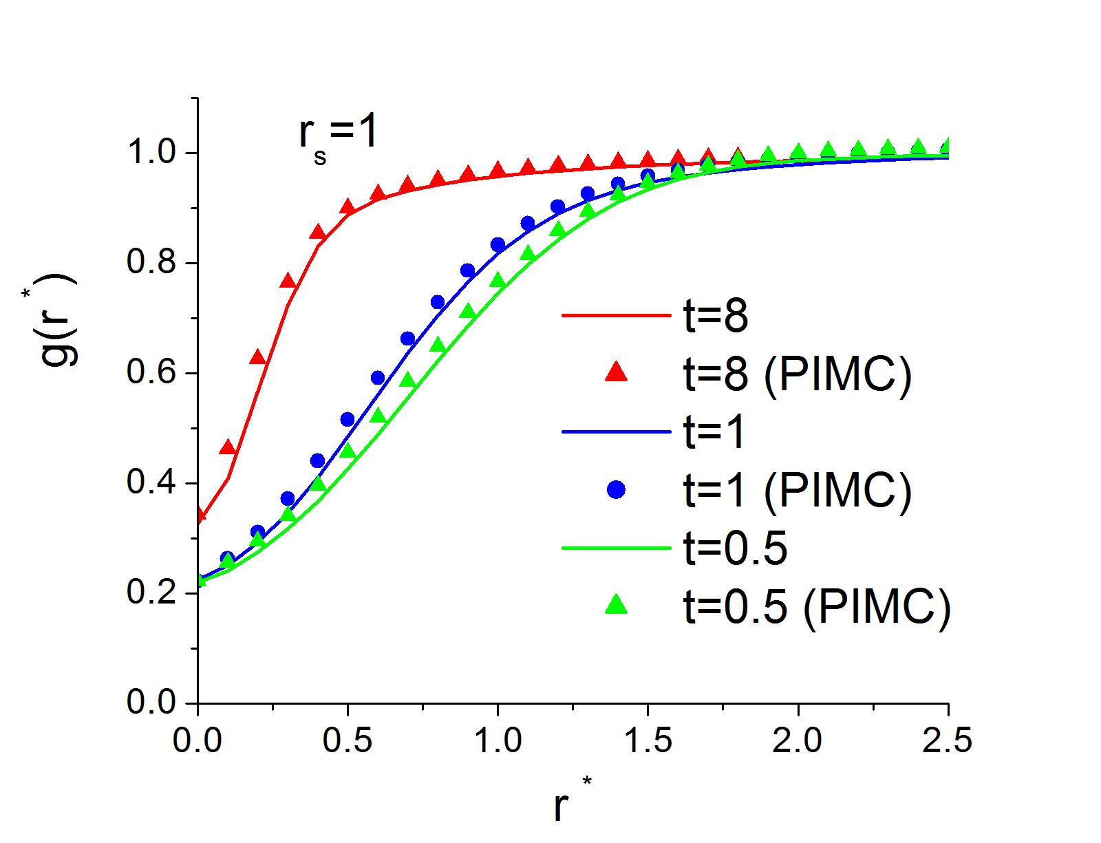
Figure 1: Pair correlation function $g(r^{*})$ for $r_{s}=1$ at $t=$ 0.5, 1, and 8.

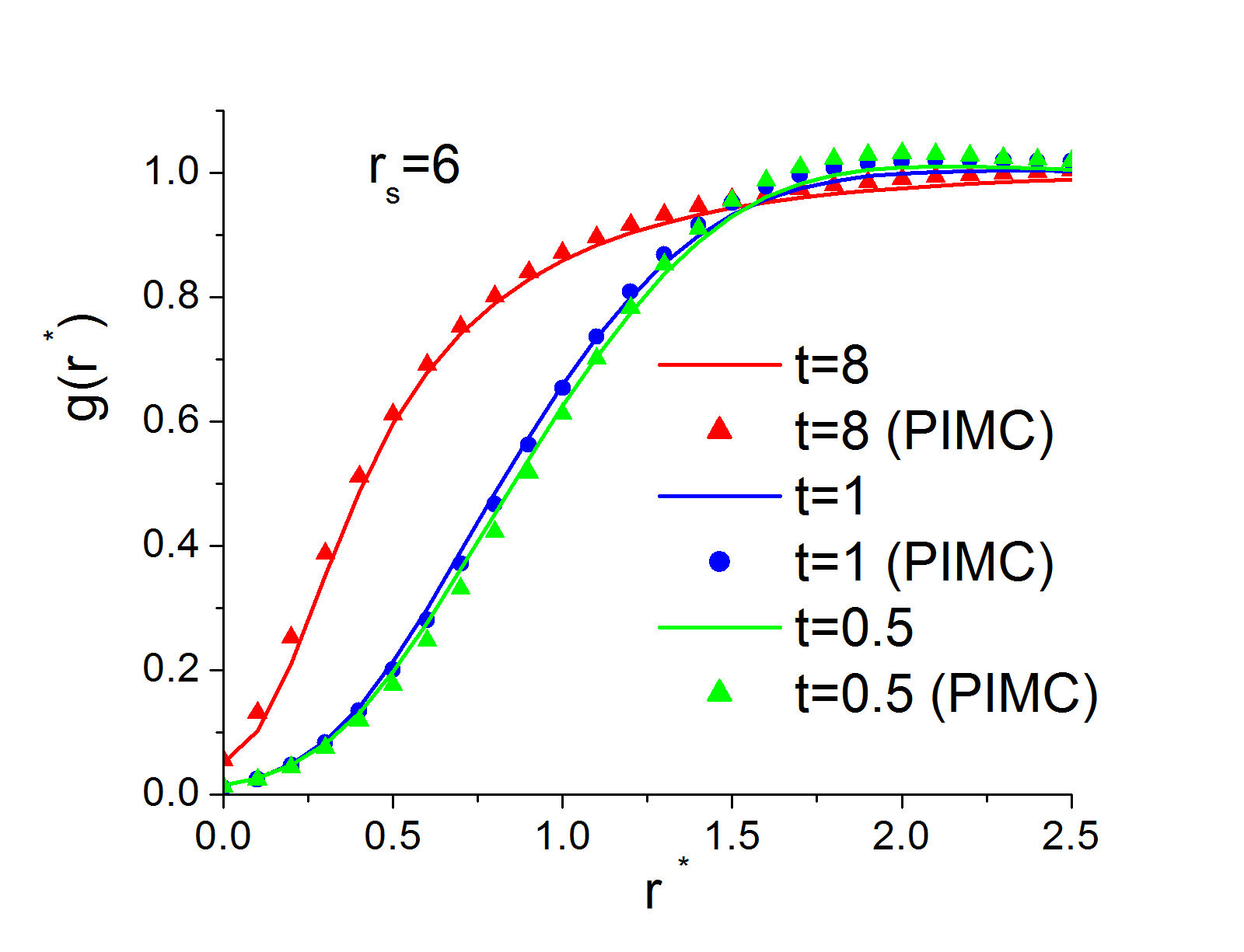
Figure 2: Pair correlation function $g(r^{*})$ for $r_{s}=6$ at $t=$ 0.5, 1, and 8.

4 Charges in a Harmonic Trap

For a second application of the classical map consider $N$ charges in a harmonic trap. The classical HNC of the last section, extended to this inhomogeneous system [13], has been shown to give an accurate description of the radial density profile for this system [14]. Of particular interest is the quantitative description of shell structure that occurs for classical strong coupling conditions. In this section, that approach is extended to include quantum effects.

The HNC theory for the density profile together with (8) and (9) leads to

$$\ln\left(n\left(\mathbf{r}\right)\lambda_{c}^{3}\right)=\beta_{c}\mu_{c}-\beta v_{c}(\mathbf{r})+\int d\mathbf{r}^{\prime}c(\left|\mathbf{r-r}^{\prime}\right|,\mu_{c},\beta_{c})n\left(\mathbf{r}^{\prime}\right).$$ (20)

Here $c(r,\mu_{c},\beta_{c})$ is the same direct correlation function as described in the previous section. Also, $v_{c}(\mathbf{r})$ is the effective classical trap which includes quantum behavior of the given harmonic trap. The approach is to determine $v_{c}(\mathbf{r})$ approximately by inverting (20) for a given approximate quantum density $n\left(\mathbf{r}\right)$. Two approximations are compared here.

The first approximation is to invert (20) for non-interacting particles in a trap. The quantum effects in this case are entirely due to exchange symmetry

$$v_{c}^{\ast(0)}(\mathbf{r}^{\ast})=c-\ln\left(n^{\ast(0)}\left(\mathbf{r}^{\ast}\right)\right)+\int d\mathbf{r}^{\ast\prime}c^{(0)}(\left|\mathbf{r}^{\ast}\mathbf{-r}^{\ast\prime}\right|,r_{s},t)n^{\ast(0)}\left(\mathbf{r}^{\ast\prime}\right).$$ (21)

Here $v_{c}^{\ast}(\mathbf{r}^{\ast})\equiv$ $\beta_{c}v_{c}(\mathbf{r})$ and the superscript $0$ on a property denotes its ideal gas value. Also, $c$ is a constant that only sets the normalization of the density profile. The calculation of $n^{\ast(0)}\left(\mathbf{r}^{\ast}\right)$ is straightforward in terms of the harmonic oscillator eigenfunctions, but for the case considered here $\left(N=100\right)$ it is found that the local density approximation (finite temperature Thomas-Fermi) is quite accurate. An important qualitative feature of $n^{\ast(0)}\left(\mathbf{r}^{\ast}\right)$ is its vanishing at a finite $\mathbf{r}^{\ast}$ as $t\rightarrow 0$. This leads to the formation of a hard wall in the effective classical trap. It is well known that such hard walls produce shell structure in classical mechanics, so this represents a quantum origin for new shell structure independent of Coulomb correlations.

The second approximation is to invert (20) with mean field quantum Coulomb correlations

$$v_{c}^{\ast(H)}(\mathbf{r}^{\ast})=c-\ln\left(n^{\ast(H)}\left(\mathbf{r}^{\ast}\right)\right)+\int d\mathbf{r}^{\ast\prime}\left(c^{(0)}(\left|\mathbf{r}^{\ast}\mathbf{-r}^{\ast\prime}\right|,r_{s},t)-\frac{\Gamma\left(t,r_{s}\right)}{\left|\mathbf{r}^{\ast}\mathbf{-r}^{\ast\prime}\right|}\right)n^{\ast(H)}\left(\mathbf{r}^{\ast\prime}\right).$$ (22)

The density $n^{\ast(H)}\left(\mathbf{r}^{\ast}\right)$ is calculated from quantum density functional theory without exchange or correlation (Hartree approximation), and again using the local density approximation. It gives a qualitative change from the ideal gas form (21) since the system is considerably expanded by the Coulomb repulsion. The hard wall is mitigated and resulting effective classical trap potential has a more harmonic form.

Figure 3 shows the density profiles obtained from (20) using (21) or (22). It is seen that the strong shell structure from the ideal gas hard wall is removed when Coulomb interactions are included. Also shown on this figure are the effective classical trap potentials for the two cases. The result from (21) shows a kink which is a precursor of the hard wall at $t=0$. Although this deviation from harmonic is small, it is sufficient to generate a large shell. In contrast, the result from (22) is more nearly harmonic and has only the shell due to Coulomb correlations already present in the purely classical calculation (no quantum effects) [14]. The lesson from this comparison is that quantum effects on the effective classical trap potential determined without Coulomb interactions lead to a false mechanism for shell structure. The more realistic mean field quantum determination does not have this shell structure and provides a quite different density profile. A more complete discussion of this comparison and results for a wide range of $r_{s},t$ will be given elsewhere [15].

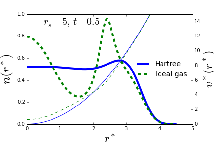
Figure 3: Density profiles (thick lines) and effective classical trap potentials (thin lines) using the Hartree and ideal gas approximations.

5 Discussion

The use of an effective classical system to describe quantum effects has been shown to provide a practical tool by the two examples of the previous sections. Although the results are quite good for the methods used here to determine the effective pair potential and trap potential, and the HNC implementation of the classical statistical mechanics, improvements in both remain to be explored. For example, the limitations of the HNC theory can be eliminated using these same potentials in molecular dynamics or Monte Carlo simulations.

The comparisons of the last section show that incorrect results can be obtained if the input quantum mechanics for the effective potentials is not sufficiently representative of the real system. For the electron gas, the effective potential has a Coulomb tail whose amplitude is constrained to satisfy an exact sum rule. It would be useful to have exact constraints for other systems as well, to assure applicability over a wide range of the parameter space.

As noted in the introduction, there is strong current interest in systems of electrons and ions to describe conditions of warm, dense matter [1]. Such systems are described by molecular dynamics simulation of the ions whose forces are calculated from a density functional theory (DFT) for the electrons at each time step. Traditionally, the DFT calculation is performed within the Kohn-Sham approach requiring a self-consistent diagonalization of an effective single electron Hamiltonian to construct the local density. At temperatures approaching the Fermi temperature, the number of relevant states (orbitals) becomes large and the calculations are no longer practical. A resolution of this problem is to forgo the Kohn-Sham method and return to the original form of DFT with a single Euler equation for the local density determined from the free energy as a known functional of the density. The primary difficulty is finding the non-interacting free energy as a functional of the density, which remains an unsolved problem in the quantum theory. However, its classical counterpart does not have this difficulty – the non-interacting free energy is known as an explicit functional of the density. Hence, an implementation of the effective classical system as described here, together with classical DFT, provides the desired orbital free DFT.

To see how this might be implemented consider a system of $N_{e}$ electrons and $N_{i}$ positive ions with charges $Z$ and positions $\left\{\mathbf{R}_{\alpha}\right\}$. For charge neutrality $N_{i}Z=N_{e}$. This can be viewed as an electron system in the external potential of the ions

$$v(\mathbf{r})=\sum_{\alpha=1}^{N_{i}}\frac{-Ze^{2}}{\left|\mathbf{r}-\mathbf{R}_{\alpha}\right|}\;.$$ (23)

Return to (20) for the corresponding local electron density, where now $v_{c}(\mathbf{r})$ is the effective classical potential corresponding to (23). A reasonable, realistic determination of $v_{c}(\mathbf{r})$ might be given by (22) in the form

$$v_{c}^{\ast(HF)}(\mathbf{r}^{\ast}) =c-\ln\left(n^{\ast(HF)}\left(\mathbf{r}^{\ast}\right)\right)$$

$$\qquad+\int d\mathbf{r}^{\ast\prime}\left(c^{(0)}(\left|\mathbf{r}^{\ast}\mathbf{-r}^{\ast\prime}\right|,r_{s},t)-\frac{\Gamma\left(t,r_{s}\right)}{\left|\mathbf{r}^{\ast}\mathbf{-r}^{\ast\prime}\right|}\right)n^{\ast(HF)}\left(\mathbf{r}^{\ast\prime}\right),$$ (24)

where now $n^{\ast(HF)}\left(\mathbf{r}^{\ast}\right)$ is the Hartree-Fock electron density for the given array of electrons. While determination of $n^{\ast(HF)}\left(\mathbf{r}^{\ast}\right)$ is still non-trivial it is a practical problem, and then use of $v_{c}^{\ast(HF)}(\mathbf{r}^{\ast})$ in (20) gives the desired orbital free DFT for the electrons.

Dharma-wardana has proposed a more complete application of the classical DFT for both the electrons and ions [7], eliminating the molecular dynamics simulation for the ions. An additional effective classical electron - ion potential must be determined in this case.

6 Acknowledgments

The authors are indebted to Michael Bonitz for his comments and criticism of an earlier ms. This research has been supported in part by NSF/DOE Partnership in Basic Plasma Science and Engineering award DE-FG02-07ER54946 and by US DOE Grant DE-SC0002139.

References

- [1] V. Karasiev, T. Sjostrom, D. Chakraborty, J. W. Dufty , F. E. Harris , K. Runge, and S. B. Trickey, Innovations in Finite-Temperature Density Functionals, Chapter in Computational Challenges in Warm Dense Matter, edited by F. Graziani et al. (Springer Verlag) in print; R.P. Drake,”High Energy Density Physics”, Phys. Today 63, 28-33 (2010) and refs. therein; Basic Research Needs for High Energy Density Laboratory Physics (Report of the Workshop on Research Needs, November 2009), U.S. Department of Energy, Office of Science and National Nuclear Security Administration, 2010, see Chapt. 6 and references therein.
- [2] M. Allen and D. Tildesley, Computer simulation of liquids. Oxford University Press, NY, 1989).
- [3] J. Lutsko, Recent Developments in Classical Density Functional Theory, Adv. Chem. Phys. 144, S. Rice, ed. (J. Wiley, Hoboken, NJ, 2010).
- [4] J-P Hansen and I. MacDonald, Theory of Simple Liquids, (Academic Press, London, 2006).
- [5] see for references C. Jones and M. Murillo, ”Analysis of semi-classical potentials for molecular dynamics and Monte Carlo simulations of warm dense matter”, High Energy Density Physics 3 (3), 397 (2007).
- [6] F. Perrot and M. W. C. Dharma-wardana, ”Spin-polarized electron liquid at arbitrary temperatures: Exchange-correlation energies, electron-distribution functions, and the static response functions”, Phys. Rev. B 62 16536 (2000).
- [7] M. W. C. Dharma-wardana, ”The classical-map hyper-netted-chain (CHNC) method and associated novel density-functional techniques for warm dense matter”, Int. J. Quantum Chem. 112 53 (2012); M. W. C. Dharma-wardana, ”Strongly-Coupled Coulomb Systems using finite-T Density Functional Theory: A review of studies on Strongly-Coupled Coulomb Systems since the rise of DFT and SCCS-1977”, Contrib. Plasma Phys. (2014, to be published; http://arxiv.org/abs/1412.6811).
- [8] Y. Liu and J. Wu, ”A bridge-functional-based classical mapping method for predicting the correlation functions of uniform electron gases at finite temperature”, J. Chem. Phys. 140, 084103 (2014).
- [9] J. W. Dufty and S. Dutta, ”Classical Representation of a Quantum System at Equilibrium”, Contrib. Plasma Phys. 52 100 (2012); ”Classical representation of a quantum system at equilibrium: Theory”, Phys. Rev. E 87 032101 (2013).
- [10] S. Dutta and J. Dufty, ”Classical representation of a quantum system at equilibrium: Applications”,Phys. Rev. E 87, 032102 (2013).
- [11] E. Brown, B. Clark, J. DuBois, and D. Ceperley, ”Path-Integral Monte Carlo Simulation of the Warm Dense Homogeneous Electron Gas”, Phys. Rev. Lett. 110 146405 (2013).
- [12] S. Dutta and J. Dufty, ”Uniform electron gas at warm, dense matter conditions”, Euro. Phys. Lett., 102 67005 (2013).
- [13] P. Attard, ”Spherically inhomogeneous fluids. I. Percus Yevick hard spheres: Osmotic coefficients and triplet correlations”, J. Chem. Phys. 91, 3072 (1989).
- [14] J. Wrighton, J. W. Dufty, H. Kählert, and M. Bonitz, ”Theoretical description of Coulomb balls: Fluid phase”, Phys. Rev. E 80, 066405 (2009); J. Wrighton, J. W. Dufty, M. Bonitz, and H. Kählert, ”Shell Structure of Confined Charges at Strong Coupling”, Contrib. Plasma Phys. 50, 26 (2010).
- [15] J. Wrighton, J. W. Dufty, and S. Dutta (in progress).