Bicep2/ Keck Array IV: Optical Characterization and Performance of the Bicep2 and Keck Array Experiments

Abstract

Bicep2 and the Keck Array are polarization-sensitive microwave telescopes that observe the cosmic microwave background (CMB) from the South Pole at degree angular scales in search of a signature of inflation imprinted as B-mode polarization in the CMB. Bicep2 was deployed in late 2009, observed for three years until the end of 2012 at 150 GHz with 512 antenna-coupled transition edge sensor bolometers, and has reported a detection of B-mode polarization on degree angular scales. The Keck Array was first deployed in late 2010 and will observe through 2016 with five receivers at several frequencies (95, 150, and 220 GHz). Bicep2 and the Keck Array share a common optical design and employ the field-proven Bicep1 strategy of using small-aperture, cold, on-axis refractive optics, providing excellent control of systematics while maintaining a large field of view. This design allows for full characterization of far-field optical performance using microwave sources on the ground. Here we describe the optical design of both instruments and report a full characterization of the optical performance and beams of Bicep2 and the Keck Array at 150 GHz.

1. Introduction

Inflation is a theory that describes the entire observable universe as a microscopic volume that underwent violent, exponential expansion during the first tiny fraction of a second (see Planck Collaboration (2014b) for a review). Inflation is supported by the flatness and uniformity of the universe observed through measurements of the cosmic microwave background (CMB). A generic prediction of inflation is the production of a gravitational-wave background, which in turn would leave a faint imprint in the polarization pattern of the CMB in addition to the already detected curl-free “E-mode” polarization sourced by density fluctuations at last scattering. A component of the inflationary signature would be a unique, divergence-free, “B-mode” polarization pattern at large angular scales. The strength of the B-mode polarization signature depends on the energy scale of inflation, and could be detectable if inflation occurred near the energy scale of grand unification, $\sim 10^{16}$ GeV (Seljak, 1997; Kamionkowski et al., 1997; Seljak & Zaldarriaga, 1997).

Bicep2 and the Keck Array are microwave polarimeters that observe the CMB from the South Pole in search of a B-mode polarization signature from inflation (Ogburn IV et al., 2010; Sheehy et al., 2010; BICEP2 Collaboration, 2014a). The receivers use a compact, on-axis refracting telescope design to couple radiation into a detector array of 512 antenna-coupled transition edge sensor (TES) bolometers. Bicep2 and the Keck Array leverage field-proven techniques employed for the Bicep1 telescope (Keating et al., 2003), but with a vastly increased number of detectors, leading to increased sensitivity to the tiny B-mode polarization signal. Bicep2 has 512 detectors and the Keck Array has 2560 detectors in the 150 GHz-only configuration used in 2012 and 2013.

Table 1 shows the changes in configuration for Bicep2 and the Keck Array between observing seasons presented in this paper. The Bicep2 experiment observed for three years at 150 GHz from 2010 through 2012 and reported a detection of B-mode polarization on degree angular scales (BICEP2 Collaboration, 2014b). All five Keck Array receivers were installed and operational beginning with the 2012 observing season. For the 2012 and 2013 observing seasons, the Keck Array had five receivers at 150 GHz. Two of the Keck Array receivers were configured to observe at 95 GHz beginning with the 2014 observing season, and two more receivers have been configured to observe at 220 GHz for the 2015 observing season. Bicep2 observes from the Dark Sector Laboratory (DSL), and the Keck Array observes from a separate observing platform and telescope mount in the Martin A. Pomerantz Observatory (MAPO). The two observatories are situated approximately 200 m apart. Here we report on beam characterization for Bicep2 and the 2012 and 2013 observing seasons of the Keck Array.

This paper is one in a series of publications by the Bicep2 and Keck Array collaborations. In this paper, we hereafter refer to other publications in this series as the Results Paper (BICEP2 Collaboration, 2014b), the Instrument Paper (BICEP2 Collaboration, 2014a), the Systematics Paper (BICEP2 Collaboration, 2015), and the Detector Paper (BICEP2, Keck Array, and Spider Collaborations, 2015).

The Systematics Paper discusses in detail the level of contamination present in the Bicep2 analysis presented in the Results Paper. The most significant systematic challenge arises from differential beam effects present in the Bicep2 and Keck Array instruments. Differential beam effects between co-located orthogonally polarized pairs of detectors can lead to leakage of the CMB temperature signal into the much smaller polarization signal. It is therefore crucial that we fully understand the optical system and demonstrate that the achieved sensitivity is not compromised by systematics due to beam effects.

In this paper, we describe in detail the optical design of the Bicep2 and Keck Array telescopes (Section 2). We report a characterization of the optical performance of the Bicep2 and Keck Array instruments, compare it to physical optics simulations, and discuss the level of E-mode to B-mode (E-to-B) leakage (Section 3). We then discuss the construction of per-detector beam maps, which are inputs to simulations that are used to measure temperature to polarization leakage after removal of leading order contributions to beam mismatch between co-located orthogonally polarized detectors in a pair (Section 4).

Table 1Configuration of the Bicep2 and Keck Array receivers for each year of observation presented in this paper

Receiver		Configuration
Bicep2 2010-2012		150 GHz, unchanged between observing seasons
The Keck Array 2012	Receiver 0	150 GHz
	Receiver 1	150 GHz
	Receiver 2	150 GHz
	Receiver 3	150 GHz
	Receiver 4	150 GHz
The Keck Array 2013	Receiver 0	150 GHz, unchanged
	Receiver 1	150 GHz, one of the four focal plane tiles replaced
	Receiver 2	150 GHz, unchanged
	Receiver 3	150 GHz, focal plane from Bicep2 installed
	Receiver 4	150 GHz, new focal plane installed

Figure 1.— A schematic of the Bicep2 optical chain with each optical element labeled. The relative position of the lenses and focal plane is to scale. The Keck Array optical chain is identical except that the IR-blocking filters in front of the objective lens are all on the 50 K stage in the Keck Array and the positions of the metal-mesh low pass filter and 4 K nylon filter are reversed.

2. Optical design and modeling

The Bicep2/Keck Array optical design is a compact, single frequency band (150 GHz for Bicep2 and 95, 150, or 220 GHz for the Keck Array), on-axis refractor with a 26.4 cm diameter aperture. This design is similar to that of the Bicep1 experiment (Yoon et al., 2006; Takahashi et al., 2010). The Bicep2/Keck Array optical design is schematically summarized in Figure 1 and discussed in the Instrument Paper, Aikin et al. (2010), and Vieregg et al. (2012).

In both experiments, the aperture stop, lenses, and telescope tube assembly are cooled to 4 K. The Bicep2 telescope is cooled with liquid helium to 4 K and has two vapor-cooled shields (at 40 K and 100 K respectively) as intermediate cryogenic stages, while the Keck Array telescope is cooled to 4 K using a pulse-tube cooler (Cryomech PT-410) and uses a single 50 K intermediate stage, also kept cold using the pulse-tube cooler.

The telescope tube is lined with microwave absorber (Eccosorb HR10) loaded with Stycast 2850 epoxy. This design allows for stray, reflected light to be absorbed on the walls of the telescope tube while providing minimal loading on the focal plane. The lining of the telescope tubes has low reflectivity even at shallow incidence angles, and the epoxy-loading reduces the shedding of particulate matter from the absorber.

The absorbing aperture stop is made of microwave absorber (Eccosorb AN74). In the time reversed sense, pixels in the focal plane evenly illuminate the aperture stop through the optics. The central pixels terminate at $-$12 dB from their maximum, near their first Airy null (for a description of beam shapes in the near field, see Section 3.1). The 26.4 cm aperture provides $0.5^{\circ}$ FWHM diffraction-limited resolution on the sky, which we have chosen in order to optimize the instrument to detect the peak of the primordial B-mode spectrum (at angular scales of 1–2^∘).

The compact design allows for full boresight rotation of the complete instrument. In CMB observations, we observe at multiple boresight rotation angles, which provides cancellation of a large class of systematic effects. The ability to rotate the instrument around its boresight has proven to be a powerful tool to control the level of systematics contamination below the sensitivity of the experiments.

Section 2.1 describes the antenna design, Section 2.2 describes the lens design, Section 2.3 describes the design of the infrared (IR) filters, Section 2.4 discusses the vacuum window, Section 2.5 describes the environmental membrane in front of the vacuum window, Section 2.6 discusses the ground shielding system, and Section 2.7 describes the results of the optical simulation of the system.

2.1. Antenna design

Each pixel absorbs incident radiation through a planar superconducting antenna array, shown in Figure 2. The antenna design used in Bicep2 and the Keck Array is also used in the balloon borne Spider experiment (Filippini et al., 2010), and a similar design is used in Bicep3 (Ahmed et al., 2014), which was deployed in late 2014 and will begin observation in early 2015. The design is fabricated lithographically, allowing for rapid and scalable production of detector tiles.

Microwave radiation is received by a two-dimensional array of sub-radiating slots that are spaced closely enough to avoid grating lobes at the high-frequency end of the observing band. For 150 GHz detectors, this spacing is 604 $\mu\mathrm{m}$. We interconnect the slots with lithographed microstrip line and use the slot-array layer as a ground plane to shield those lines from direct stimulation by the incident radiation. Each pixel is dual polarized, using orthogonally oriented but co-located sets of slots that function as independent antennas with independent feed networks.

We select the overall size of the antenna to match the optics in the telescope, placing the null between the main beam and the first Airy ring at the stop’s edge. For Bicep2 and the Keck Array’s 150 GHz cameras, the antenna array is 7.8 mm on a side, using a $12\times 12$ array of slots in each polarization.

By adjusting the impedance of the microstrip lines in the feed network, we could generate an arbitrary illumination pattern and control sidelobe levels. However, for simplicity of design in Bicep2 and the Keck Array, we feed power from slots uniformly in the feed network. This top-hat illumination creates $<-$12 dB sidelobes that terminate on the absorbing stop. The feed combines waves from the slots with uniform phase to create circular Gaussian beams with matching centroids between detector pairs.

After summing radiation in the feed network, power passes through the integrated band-defining filter before terminating in a lossy transmission line on a thermally isolated island also occupied by a TES bolometer. For more information on the detector design, see the Detector Paper.

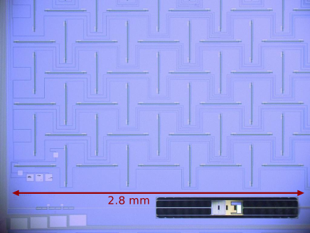
Figure 2.— A partial view of one Bicep2 dual-polarization pixel, showing the band-defining filter (lower left), TES island (lower right), and part of the antenna network and summing tree. For more information on the detector design, see the Detector Paper.

2.2. Lens design

The refracting optics consist of a pair of lenses that are cooled to 4 K and are made of high-density polyethylene (HDPE), a material with low loss and an index of refraction of 1.54 at millimeter wavelengths (Lamb, 1996). The aperture stop is coincident with the objective lens, which sits at the focus of the eyepiece lens, defining a telecentric system that makes the plate scale robust against any as-built defocus of the telescope. We chose to have only two lenses to minimize partial reflections and ghosting.

To minimize the radius of curvature of the eyepiece lens for ease of fabrication, the eyepiece lens (26.0 cm diameter) is located as far from the focal plane (18.0 cm diameter) as it can be without vignetting beams from any detectors in the focal plane. The distance to the eyepiece lens was set to 15.0 cm.

We chose the lens separation, and thus the focal length, to be 55.0 cm. This directly produces a plate scale such that the angular resolution of the telescope on the sky corresponds roughly to twice the physical separation between pixels on the focal plane, allowing us to Nyquist sample modes on the sky. Physical optics simulations performed with Zemax optical design software showed that shorter focal lengths introduced aberrations for corner detectors on the focal plane and that longer focal lengths resulted in asymmetric illumination of the aperture stop that corresponded to elliptical far-field beam patterns.

Using time-forward optics simulations with collimated ray bundles distributed in the same way as the detectors across the focal plane and incident on the objective lens at angles from $0^{\circ}$ to $8^{\circ}$ from normal incidence, we selected the objective lens geometry that minimizes the beam waist at the eyepiece lens. Analogously, we used time-reverse simulations of Gaussian-profile weighted collimated rays incident on the eyepiece lens at angles of $0^{\circ}$ to $10^{\circ}$ from normal incidence to choose the eyepiece lens geometry that minimizes the beam waist on the objective lens. We solved these iteratively in Zemax to converge on acceptable lens surface geometries. We found that while perfectly telecentric systems had good image quality, such designs illuminate the aperture asymmetrically and can induce far-field ellipticity. We ultimately sacrificed telecentricity to attain symmetric far-field beams.

We anti-reflection (AR) coated the Bicep2/Keck Array lenses with porous Teflon (Mupor) whose index of refraction and thickness were customized to tune the performance to the observing frequency of each receiver given the optical material being AR coated. The AR coating was attached to each optical element through heat bonding using a thin film of low-density polyethylene (LDPE).

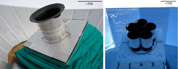
Figure 3.— A picture of Bicep2 (left) and the Keck Array (right) from the outside. The forebaffles and the reflective ground shield are visible.

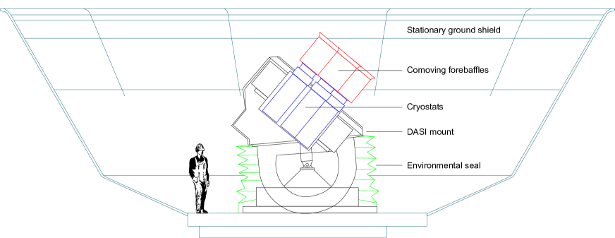
Figure 4.— Cross-sectional view of Bicep2 (top) and the Keck Array (bottom) in their observing configurations. Both experiments are shown to the same scale. The receivers are shown in blue, the forebaffles are shown in red, and the environmental seals are shown in green. Also shown are the mounts and the stationary ground shields.

2.3. Filter stack

Teflon, nylon, and a metal-mesh low-pass filter block IR radiation from reaching the focal plane. Teflon has excellent in-band transmission at cryogenic temperatures. While nylon has higher in-band transmission loss, it has a steeper transmission rolloff out of band, providing significant reduction of far-IR loading on the sub-kelvin stages. The metal-mesh filter is a low-pass filter with a cutoff at 250 GHz, providing additional blocking of out-of-band power (Ade et al., 2006).

In Bicep2 and the Keck Array, two Teflon filters and one nylon filter sit in front of the objective lens. In Bicep2, one Teflon filter is held at 100 K and the second Teflon filter and the nylon filter are held at 40 K, while in the Keck Array they are all on the 50 K stage. In both experiments, a nylon filter and the low-pass metal-mesh filter sit at 4 K between the objective and eyepiece lenses inside the telescope itself to further reduce loading. We AR coat all filters using the same process described for AR coating the lenses in Section 2.2.

2.4. Vacuum window

The Bicep2/Keck Array vacuum window has a 32 cm clear aperture, making design and construction of strong and durable windows a challenge. The Bicep2 vacuum window was made of Zotefoam PPA30, a dry nitrogen-expanded polypropylene foam chosen for its high microwave transmission, its strength against deflection under vacuum, its adhesion strength to the epoxy used to bond the foam to an aluminum frame, and its previous successful use in similar applications (Runyan et al., 2003; Takahashi et al., 2010). The 10 cm thick window was made of four layers of PPA30 joined together by heat lamination and was bonded to an aluminum frame using Stycast 1266 epoxy. We measured the transmission of the Bicep2 window to exceed 98% at 150 GHz, consistent with the Bicep1 window (Takahashi et al., 2010).

Keck Array windows are made of Zotefoam HD30 because Zotefoam ceased production of PPA30. HD30 is a nitrogen-expanded polyethylene foam that has similar performance to PPA30 in both microwave transparency and mechanical strength, with slightly inferior lamination and adhesion qualities. Keck Array windows are composed of layers of HD30 joined together by heat lamination, like the Bicep2 window. The vacuum windows for the 2012 and 2013 observing seasons were bonded to their aluminum frames using Stycast 2850 epoxy. After the 2012 observing season, we increased the thickness of the windows to 12 cm (the maximum possible with a four layer HD30 laminate) because we observed the vacuum window foam tearing away from the epoxy used to attach the foam to the aluminum frame. The $\lesssim 2\%$ transmission loss appears to be dominated by the laminations, so maintaining four layers while increasing the thickness has had minimal impact on performance, while the thicker windows are able to withstand the force from the vacuum over time.

2.5. Membrane

In front of the window sits a thin transparent membrane held tautly by two aluminum rings. The membrane creates an environmental shield to protect the window from snow. The enclosed space between the membrane and the window is slightly pressurized with dry nitrogen gas to prevent condensation on the foam window. Room-temperature air flows through holes in the aluminum ring onto the top of the membrane so that any snow that accumulates sublimates away.

For Bicep2, the initially deployed membrane was 0.5 mil thick Mylar, which has low reflectivity at 150 GHz (0.2%). In April 2011, the membrane was replaced with 0.9 mil biaxially oriented polypropylene (BOPP) and the pressure of the nitrogen was adjusted to reduce vibrations in the membrane, discussed in the Instrument Paper. The Keck Array uses the same BOPP membranes as Bicep2.

2.6. Baffling and ground shielding

A co-moving ground shield, called the forebaffle, installed in front of each receiver’s vacuum window reduces sidelobe pickup. The forebaffles for Bicep2 and the Keck Array have identical construction except for their overall sizes. The Bicep2 forebaffle was 94 cm tall and 71 cm in diameter, and the Keck Array forebaffles used for the five-receiver configuration (2012 and later) are 74 cm tall and 64 cm in diameter. The forebaffles have rolled lips at the upper edge of the cylinder to reduce diffraction and diffuse any far-sidelobe beams. We coat the inside of the forebaffle with Eccosorb HR10 microwave absorber and Volara, a weatherproofing foam, to terminate the sidelobes while only modestly increasing thermal loading on the focal plane. The forebaffles intersect radiation at $9.5^{\circ}$ from the telescope boresight axis as measured from the edge of the vacuum window. The forebaffles and ground shield for Bicep2 and the Keck Array are shown in the photographs in Figure 3 and in cross-sectional diagrams in Figure 4.

A fixed reflective ground shield, visible in Figure 3, redirects any stray light to the cold sky and shields the telescope from having any direct line-of-sight from the ground. The Bicep2 ground shield was previously used by Bicep1 (Takahashi et al., 2010) and the Keck Array ground shield was previously used by Dasi (Leitch et al., 2002) and Quad (Hinderks et al., 2009).

The two ground-shielding stages were designed so that at the lowest CMB observation angle (an elevation of $55^{\circ}$), the top of the fixed reflective ground shield is still $11^{\circ}$ below any direct line of sight from the telescope past the co-moving forebaffle. Additionally, as viewed from the receivers, the top of the fixed reflective ground shield is at least $15^{\circ}$ above the ground. Therefore, rays from the telescope must diffract twice (over the edge of the co-moving forebaffle and the ground shield) before they hit the ground. A drawing of Bicep2 and Keck Array receivers in their observing configurations is shown in Figure 4.

2.7. Modeled far-field beams

We have modeled the far-field beam patterns with Zemax simulations that account for optical elements between the focal plane and the aperture stop, including lenses and filters. The optical simulation is discussed more fully in Aikin et al. (2010). Figure 5 shows the simulated far-field beam pattern for the two orthogonally polarized beams in a given detector pair, which we denote “$A$” and “$B$.” The Figure shows median-radius and corner pixels in the focal plane to demonstrate beam uniformity across the focal plane. The median-radius pixel is displaced 5.6 cm from the optical axis, and the corner pixel is displaced 8.0 cm. Beams are Gaussian with a $0.5^{\circ}$ FWHM, and the Airy ring structure is clearly visible.

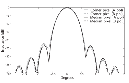
Figure 5.— Simulated far-field beam pattern for orthogonally polarized $A$ and $B$ beams, for both median-radius and corner pixels in the focal plane. Beams share the same peak normalization.

3. Optical characterization

We have fully characterized the beams of Bicep2 and the Keck Array for its 2012 and 2013 configurations. The ultimate goal of this characterization is to place constraints on the temperature to polarization leakage and the E-to-B leakage due to beam effects, as presented in the Systematics Paper.

In this Section, we first present results of near-field beam characterization studies (Section 3.1). We then discuss the far-field beam characterization campaign at the South Pole (Section 3.2), including measurements of beam shape parameters (Section 3.2.1) and differential beam parameters (Section 3.2.2) and a comparison with optical models (Section 3.2.3). Finally, we discuss power contained in far sidelobes (Section 3.3) and polarization angle and cross-polar response measurements (Section 3.4), including placing constraints on E-to-B leakage.

3.1. Near-field beam characterization

To characterize aperture illumination, we measured the near-field beam pattern of each Bicep2 and Keck Array detector. While far-field beam maps are primarily sensitive to the amplitude distribution of the electric field in the focal plane, maps made in the aperture plane of the instrument are primarily sensitive to the phase of the electric field in the focal plane. As a result, near-field maps can serve as a probe of phase gradients within the phased-array antennas. Near-field maps can also serve as a probe of secondary reflections that focus near the aperture plane and of vignetting within the telescope. The main purpose of near field measurements is to feed back into the detector and optics fabrication process for future generations of receivers.

Near-field maps were made using a chopped thermal source mounted on an x-y translation stage attached to the cryostat above the vacuum window as close to the aperture stop of the telescope as possible. In practice, the source is about 30 cm above the aperture.

Near-field maps were acquired during two consecutive summer seasons at the South Pole for Bicep2 and are acquired after the first cool down of each Keck Array receiver at South Pole. The TES detectors can operate on each of two superconducting transitions: the titanium transition, on which CMB observations are made, and the higher-temperature aluminum transition. Beam mapping data is acquired with the TES detectors on their aluminum transition, which can accommodate the higher loading present in the lab. We observe the CMB with the detectors on their titanium transition, but the beams formed for a given channel are expected to be the same for the two superconducting transitions, since beams are formed by the antenna network and the optics, not the detector itself.

Figure 6 shows the beam pattern of two example detectors in the near field for Bicep2 and the Keck Array in its 2012 configuration. In each case, the left panel shows the beam pattern of a detector near the center of a tile in the focal plane that evenly illuminates the aperture. The right panel shows the beam pattern of a detector near the edge of the focal plane that is significantly truncated by the aperture because of non-ideal beam pointing at the focal plane, which we call “beam steer.” This beam steer can be as large as 5–10^∘ in Bicep2, more than is predicted by the physical optics model presented in Section 2.7 (Aikin, 2013). This impacts not only optical throughput, but can also potentially introduce beam distortion caused by the asymmetric and aggressive illumination of the aperture stop. This type of truncation translates to moderate ellipticity in the beam pattern in the far field and only affects a small fraction of detectors that sit near the edges of tiles in the focal plane. Beam steer is typically smaller for Keck Array receivers compared to Bicep2.

As discussed in Section 4, systematic effects stemming from the observed per-beam far field ellipticity have been successfully removed in analysis to the level required for Bicep2 and the Keck Array. Although the effects of beam steer are therefore not concerning for Bicep2 and the Keck Array, reducing beam steer for future generations of detectors would increase optical throughput and reduce far field ellipticity, improving sensitivity slightly and potentially improving the achievable level of residual systematics.

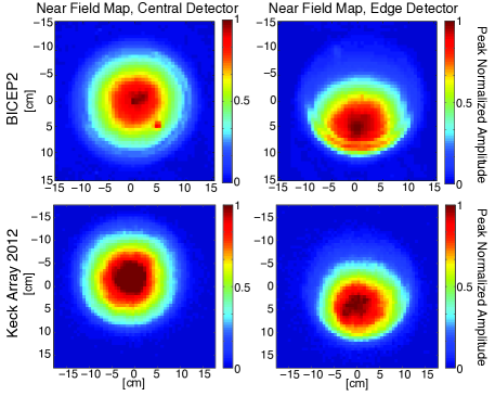
Figure 6.— A measurement of the near-field beam pattern for two example channels in Bicep2 and the Keck Array during 2012. Left: A detector near the center of a tile in the focal plane. Right: A detector near the edge of the focal plane, showing significant truncation by the aperture (worst case). This truncation leads to moderate ellipticity in the far field. The sharp feature seen for the center pixel in Bicep2 is consistent with a reflection off of the 4 K nylon filter, and is diffusely coupled to the sky.

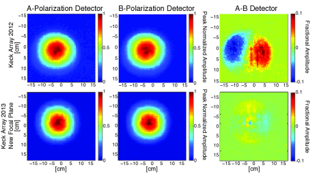
Figure 7.— An example Keck Array detector pair that shows beam mismatch in the near field. Left: The optical response of an $A$ polarization detector in a typical detector pair. Center: The optical response of the co-located $B$ polarization detector. Right: The fractional difference between the $A$ and $B$ optical response. The top panels show a typical detector pair from a focal plane in 2012, and the bottom panels show a typical detector pair from the new focal plane installed in 2013 with dramatically reduced differential pointing.

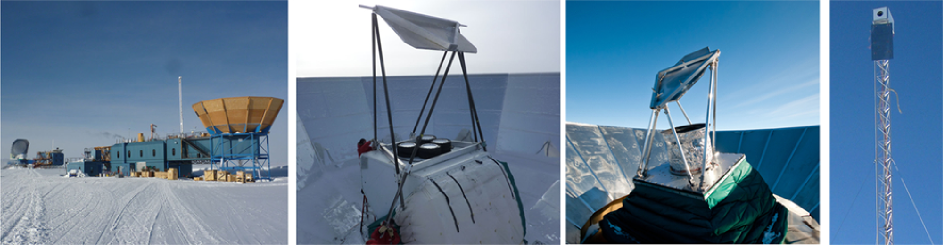
Figure 8.— The setup for measuring far-field beam patterns of Bicep2 and Keck Array detectors in situ at the South Pole. A chopped thermal source broadcasts from a mast on MAPO or DSL, and a large aluminum honeycomb mirror is installed to redirect the beams of Bicep2 and the Keck Array to the source. Left: DSL (far) and MAPO (near), home of Bicep2 and the Keck Array. Both masts are up and are being used for beam mapping. Center Left: The large mirror installed for beam mapping on the Keck Array. Center Right: The smaller mirror installed for beam mapping on Bicep2. Right: A close up of a microwave source mounted on the mast.

The sharp bright feature in the bottom right quadrant of the Bicep2 central detector map is consistent with a secondary reflection from the 4 K filters refocused into the aperture plane. This spot contains less than 0.1% of the integrated power of the main beam. Moreover, since it forms a sharp focus in the aperture plane, it must be broadly and diffusely coupled to the sky in the far field. This feature is not present in Keck Array receivers.

Figure 7 shows near-field maps for a typical orthogonally polarized co-located detector pair in the Keck Array, as well as a difference map between the two detectors in the pair. The top panels show a typical pair of detectors from a Keck Array focal plane in 2012, and the bottom panels show a typical pair from a new focal plane installed in 2013. Beams measured in the near field in Bicep2 and early Keck Array focal planes show a consistent mismatch in the $A$ and $B$ beam centroids of co-located, orthogonally polarized detector pairs. The centroid displacement is consistently co-aligned with the polarization axes of each tile, and thus also the summing tree axes. The amplitude was measured to be nearly constant across the focal plane, except for a small subset of pixels suffering from the severe beam steer illustrated in Figure 6. The observed patterns are consistent with our detector modeling, described in O’Brient et al. (2012).

Mismatch in the near-field centroids alone will not lead to any substantial far-field beam mismatch. While the beams may be displaced in the near field, the resulting angular displacement on the sky is negligible. However, non-idealities in the optics of the instrument, such as birefringence in the optics or an out-of-focus system, can serve to translate a near-field mismatch to the far field.

Detector development efforts have greatly reduced the near-field mismatch. The component of mismatch parallel to the summing trees was reduced by increasing spacing between lines of the summing tree to reduce the parasitic coupling and resulting phase errors. We have reduced the remaining phase error from residual coupling by adding phase lags to the summing tree. The additional path length corrects the residual phase step across the antenna’s mid-plane. Subsequent detector testing has shown that the source of the remaining near-field differential pointing, predominantly along the axis orthogonal to the summing trees, is related to contamination in the niobium films of the microstrip lines, producing non-constant wave speeds across the feed. The efforts to improve the matching of phased-array antenna beams in the aperture plane are described in detail in the Detector Paper. Keck Array focal planes installed in late 2012 and later have dramatically reduced near-field mismatch beginning with the 2013 observing season as a result of these efforts (see the lower panels of Figure 7).

3.2. Far-field beam characterization

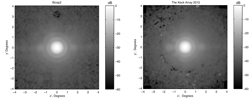
Figure 9.— Left: A map of the Bicep2 far-field response made with a thermal source, centered, rotated, and co-added over all operational channels from 2012 data. Right: A map of the Keck Array far-field response made with a thermal source, centered, rotated, and co-added over all operational channels for all 2013 Keck Array receivers. The color scale is logarithmic with decades marked in dB. The measured main beam shape and Airy ring structure are well-matched by simulations (see Section 3.2.3). Cross-talk features are evident, $1.5^{\circ}$ to the right and left of the main beam. The feature $3^{\circ}$ above the main beam in the Bicep2 is also due to crosstalk.

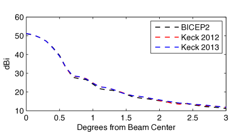
Figure 10.— Azimuthally averaged beam profiles for Bicep2 and the Keck Array for 2012 and 2013, co-added over all operational channels.

We are able to fully characterize the beam of each detector in the far field using microwave sources on the ground because the far field of the telescopes is only at a distance of 70 m. We define the far field to be a distance of $2D^{2}/\lambda$, where $D$ is the size of the aperture (26.4 cm) and $\lambda$ is the wavelength at the observing frequency of 150 GHz (2 mm).

We measure the optical response through an extensive beam mapping campaign at the South Pole. Figure 8 shows the setups used to measure the beam pattern in the far field. For beam mapping, we install flat aluminum honeycomb mirrors to redirect the beams over the top of the ground shields and to an unpolarized chopped thermal source mounted on a 10 m tall mast on MAPO (195 m away for Bicep2) or DSL (211 m away for the Keck Array). We used both a small aperture source (20 cm) and a large aperture source (45 cm) for beam characterization. These sources appear as point-like in the far field; the large aperture source subtends an angle of $0.1^{\circ}$ as viewed by the telescope, which is much smaller than the size of the beam. The thermal sources chop between a mirror directed to zenith ($\sim 15$ K) and ambient temperature ($\sim 250$ K) at a tunable frequency, set to be 18 Hz for the smaller aperture source and 10 Hz for the larger aperture source. We use maps made with these sources to study the beam shapes of each detector in order to fully understand the effects of the shape of the beams on the science data. We also made beam maps using the broad-spectrum noise source described in Section 3.4.2, which has a large and adjustable amplitude and is good for measuring relatively dim sidelobe features.

Far-field maps are made by rastering in azimuth at a scan rate of $2.0^{\circ}$ per second and stepping in elevation at a fixed boresight rotation angle. We make maps at multiple boresight rotation angles to check that a rotation of the receiver does not affect the results of the measurement. Because the effective position of the source is only $\sim 2^{\circ}$ above the horizon, and we mask out the ground when making maps, multiple boresight angles allow more thorough mapping of the response at large angles from the center of the beam. All measurements are made with the detectors on the aluminum transition. We take beam map data at a high sampling rate (150 Hz), filter the chop reference signal to match the filtering that occurs in the readout system, and then demodulate the timestream data. The reflection off of the mirror and parallax effects are handled with a pointing model that describes the Bicep2 and Keck Array mount systems as well as the mirrors used for beam mapping (Aikin, 2013).

Figure 9 shows maps of the far-field response of Bicep2 and the Keck Array in its 2013 configuration, centered, rotated, and co-added over all operational channels. The maps have been rotated before co-addition to account for the boresight angle rotation and the clocking of Keck Array receivers in the drum on the mount so that co-added maps are fixed to focal plane coordinates. The measured main beam shape and Airy ring structure are well-matched by simulations (see Section 3.2.3), and cross-talk features are evident in the stacked maps ($1.5^{\circ}$ from the main beam), corresponding to the location of the nearest neighbor detector in the multiplexing readout scheme. Figure 10 shows the azimuthally averaged beam profile for Bicep2 and the Keck Array in its 2012 and 2013 configurations, derived from the co-added maps.

From these measurements, we extract beam shape parameters on a per-detector basis and characterize the difference in the beams between detectors in each detector pair.

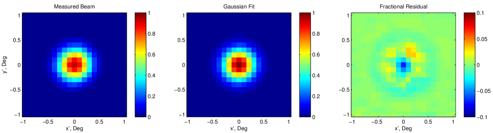
Figure 11.— Left: Example measured far-field beam pattern from Bicep2, linear scale. Middle: Gaussian fit to measured beam pattern. Right: Fractional residual after subtracting the Gaussian fit in the middle panel. The residual represents the portion of the beam that is not mitigated with the deprojection technique discussed in Section 4. Note: The right-hand panel has a different color scale than the left two panels.

Table 2Measured detector-pair beam parameters for Bicep2 and Keck Array receivers for 2012 and 2013

Receiver		Beam Parameter
		Beam Width, $\sigma_{i}$ (degrees)	Ellipticity Plus, $p_{i}$ ($+$)	Ellipticity Cross, $c_{i}$ ($\times$)
Bicep 2		$0.220\pm 0.004\pm 0.002$	$0.01\pm 0.03\pm 0.02$	$0.00\pm 0.02\pm 0.01$
Keck 2012	Receiver 0	$0.216\pm 0.003\pm 0.002$	$0.01\pm 0.03\pm 0.01$	$0.01\pm 0.02\pm 0.01$
	Receiver 1	$0.215\pm 0.004\pm 0.002$	$0.01\pm 0.02\pm 0.02$	$0.02\pm 0.02\pm 0.01$
	Receiver 2	$0.217\pm 0.004\pm 0.002$	$0.01\pm 0.03\pm 0.01$	$0.01\pm 0.02\pm 0.02$
	Receiver 3	$0.217\pm 0.004\pm 0.002$	$0.01\pm 0.02\pm 0.01$	$0.01\pm 0.02\pm 0.02$
	Receiver 4	$0.217\pm 0.004\pm 0.002$	$0.01\pm 0.02\pm 0.01$	$0.02\pm 0.02\pm 0.02$
	All receivers	$0.216\pm 0.004\pm 0.002$	$0.01\pm 0.02\pm 0.01$	$0.01\pm 0.02\pm 0.02$
Keck 2013	Receiver 0	$0.218\pm 0.004\pm 0.002$	$0.01\pm 0.03\pm 0.01$	$0.01\pm 0.02\pm 0.02$
	Receiver 1	$0.215\pm 0.004\pm 0.002$	$0.01\pm 0.02\pm 0.02$	$0.01\pm 0.02\pm 0.02$
	Receiver 2	$0.218\pm 0.004\pm 0.002$	$0.01\pm 0.03\pm 0.02$	$0.01\pm 0.02\pm 0.02$
	Receiver 3	$0.218\pm 0.005\pm 0.003$	$0.01\pm 0.03\pm 0.02$	$0.00\pm 0.02\pm 0.02$
	Receiver 4	$0.211\pm 0.002\pm 0.002$	$0.00\pm 0.02\pm 0.02$	$0.01\pm 0.02\pm 0.02$
	All receivers	$0.216\pm 0.005\pm 0.002$	$0.01\pm 0.03\pm 0.02$	$0.01\pm 0.02\pm 0.02$

3.2.1 Beam shape parameters

To facilitate parameterization of the beams, we first define a coordinate system that is fixed to the focal plane as projected onto the sky for each of the Bicep2 and Keck Array receivers. We scan the telescope in azimuth and step in elevation, and convert the angular offset between the boresight and the direction to the beam mapping source into this coordinate system.

A pixel, $P$, which has two orthogonally polarized detectors, is defined to be at a location $(r,\theta)$ from the boresight, $B$. We define $r$ as the radial distance away from the boresight and $\theta$ as the counterclockwise angle looking out from the telescope towards the sky from the $\theta=0^{\circ}$ ray (along the boresight), which is defined to be the great circle that runs between Tile 1 and Tile 2 on the focal plane. Tiles are numbered counterclockwise looking directly down on the focal plane, and Tile 1 and Tile 2 are physically located on the side of the focal plane that connects to the heatstraps to the sub-kelvin refrigerator.

We then define an ($x^{\prime}$,$y^{\prime}$) coordinate system locally for each pixel $P$. The positive $x^{\prime}$ axis is defined to be along the great circle that passes through the point $P$ that is an angle $-\theta$ from the $\hat{r}$ direction of the pixel (back toward $B$). The $y^{\prime}$ axis is defined as the great circle that is $+90^{\circ}$ away from the $x^{\prime}$ axis. The ($x^{\prime}$,$y^{\prime}$) coordinate system is then projected onto a plane at $P$.

This coordinate system is fixed to the instrument and rotates on the sky with the boresight rotation angle, also called the deck angle $K$, and the angle at which each receiver is clocked with respect to the $K=0$ line, also called the drum angle $K^{\prime}$. For Bicep2, $K^{\prime}=0$. Each Keck Array receiver has a $K^{\prime}$ rotated by $\sim 72^{\circ}$ from its two neighboring receivers in the 2012 and 2013 configurations.

A two-dimensional elliptical Gaussian is parametrized by six parameters: the gain, the two-parameter position of the center of the beam, and three parameters that together describe the beam width and the ellipticity. We fit a two-dimensional elliptical Gaussian profile to the main beam of each detector in Bicep2 and the Keck Array in a flat sky approximation, according to

$$B(\mathbf{x})=\frac{1}{\Omega}e^{-\frac{1}{2}(\mathbf{x}-\boldsymbol{\mu})^{T}\Sigma^{-1}(\mathbf{x}-\boldsymbol{\mu})}$$ (1)

where $\mathbf{x}$ is the location of the beam center, $\boldsymbol{\mu}$ is the origin, $\Omega$ is the normalization factor, and $\Sigma$ is the covariance matrix. A common parameterization for $\Sigma$ uses the widths along the major and minor axis, $\sigma_{maj}$ and $\sigma_{min}$, and the rotation angle of the major axis away from the $x^{\prime}$ axis, $\phi$. Here we have

$$\Sigma=R^{-1}CR,$$ (2)

where

$$C=\left(\begin{array}[]{cc}\sigma_{maj}^{2}&0\\ 0&\sigma_{min}^{2}\end{array}\right),$$ (5)

and the rotation matrix, $R$, is described as

$$R=\left(\begin{array}[]{cc}\cos\phi&\sin\phi\\ -\sin\phi&\cos\phi\end{array}\right).$$ (8)

We then define the ellipticity as

$$e=\frac{\sigma_{maj}^{2}-\sigma_{min}^{2}}{\sigma_{maj}^{2}+\sigma_{min}^{2}}.$$ (9)

The ellipticity alone does not specify the direction of the major or minor axis. As in the Systematics Paper, instead of using $\sigma_{maj}$, $\sigma_{min}$, and $\phi$ to describe the beam, we introduce the parameters $\sigma$, $p$, and $c$ to describe the beam width and ellipticity in the “plus” and “cross” directions respectively. In this basis, we have

$$\sigma^{2}=\frac{\sigma_{maj}^{2}+\sigma_{min}^{2}}{2}$$ (10)

and

$$\Sigma=\left(\begin{array}[]{cc}\sigma^{2}(1+p)&c\sigma^{2}\\ c\sigma^{2}&\sigma^{2}(1-p)\end{array}\right).$$ (11)

$p$ and $c$ are related to $\sigma_{maj}$, $\sigma_{min}$, and $\phi$ by

$$c=\frac{\sigma_{maj}^{2}-\sigma_{min}^{2}}{\sigma_{maj}^{2}+\sigma_{min}^{2}}\sin 2\phi,$$ (12)

and

$$p=\frac{\sigma_{maj}^{2}-\sigma_{min}^{2}}{\sigma_{maj}^{2}+\sigma_{min}^{2}}\cos 2\phi.$$ (13)

An elliptical Gaussian with its major axis oriented along the $x$-axis or the $y$-axis has a purely $+p$ or $-p$ ellipticity, while an elliptical Gaussian oriented diagonally ($\pm 45^{\circ}$) has a purely $\pm c$ ellipticity. The total ellipticity is

$$e=\sqrt{p^{2}+c^{2}}.$$ (14)

Using this parameterization, differential beam parameters for a pair of co-located orthogonally polarized detectors may be defined simply by taking the difference between the beam parameters of the two detectors. There is a straightforward relationship between parameters calculated in this way and the first order terms of a power series expansion of a Gaussian. This relates the modes that are removed from the real data through deprojection directly to the difference beam parameters obtained from beam map measurements, as discussed in the Systematics Paper.

Figure 11 shows an example map from Bicep2, the elliptical Gaussian fit, and the fractional residual after subtracting the fit. Beams and their fits for the Keck Array are similar (Vieregg et al., 2012). Table 2 shows the median value of the relevant beam parameters for each receiver in each experiment, as well as the detector-to-detector scatter (taken to be half of the width of the central 68% of the distributon of median values for each detector) and the median measurement uncertainty for individual detectors (the median over all detectors of half of the width of the central 68% of the distribution of measurements for a given detector).

The measured values in the table come from beam maps made using a chopped thermal source in the far field. The per-detector pair parameters for Bicep2 are calculated as a combination of the elliptical Gaussian fits to 24 beam maps with equal boresight rotation coverage. Each measurement of each detector’s main beam must pass a set of criteria to be included in the final extraction of beam parameters, including a check that the beam center was not near the edge of the mirror and excluding measurements where the initial elliptical Gaussian fit failed. The Keck Array beam parameters for 2012 and 2013 are obtained from independent sets of beam maps taken in February 2012 and February 2013 respectively. The maps were taken using a chopped thermal source in the far field. We separately characterize each Keck Array receiver for 2012 and 2013 because of the changes made to the receivers between the two observing seasons (see Table 1).

The absolute detector gain calibration as well as each detector’s absolute pointing information come from calibrating against CMB temperature maps from Planck (Planck Collaboration, 2014a; Planck HFI Core Team, 2011), as discussed in the Instrument Paper. We do not obtain measurements of the absolute gain of each detector from the beam maps since we use the aluminum transition and a bright source. We also do not make the final pointing measurements of each detector using the beam map data; instead, we obtain them directly from CMB maps.

Figures 12 and 13 show the distribution of each detector’s ellipticity across the focal plane for Bicep2 and the Keck Array in its 2012 and 2013 configurations. There are two effects that contribute to the observed ellipticity pattern across the focal plane. First, because our optical design places its optimal focus on an annulus of detectors a median distance from the center of the focal plane, ellipticity is induced for detectors near the edge of the focal plane. This effect is predicted by our optical simulations. Second, the beam steer effects that we observe in near field maps (described in Section 3.1) also lead to enhanced ellipticity for detectors near the edges of tiles in the focal plane. Although optical simulations do not predict the beam steer effects seen in the near field, given the observed beam steer optical simulations do predict the observed enhanced ellipticity in the far field. The net effect in the far field is a combination of the two effects, which leads to detectors near the edges of tiles and near the edge of the focal plane displaying higher ellipticity.

Figure 14 shows the per-detector beam width $\sigma$ for Bicep2 and the Keck Array. The median beam width over the focal plane is $0.220\pm 0.002\pm 0.001^{\circ}$ for Bicep2, $0.216\pm 0.004\pm 0.002^{\circ}$ for Keck Array receivers in 2012, and $0.216\pm 0.005\pm 0.002^{\circ}$ for Keck Array receivers in 2013, where the errors quoted are the detector-to-detector scatter followed by the measurement uncertainty for individual detectors (as in Table 2). The beam widths for each Keck Array receiver are consistent from one receiver to another. The slight difference in the placement of the objective lens between Bicep2 and the Keck Array could explain the difference in the beam widths between the Keck Array and Bicep2.

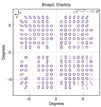
Figure 12.— Per-detector beam ellipticity for Bicep2 as projected onto the sky. The ellipticity for each detector has been exaggerated for visibility, as shown in the legend. $A$ and $B$ beams are shown in red and blue, respectively, and light colors show detectors that are not used in analysis.

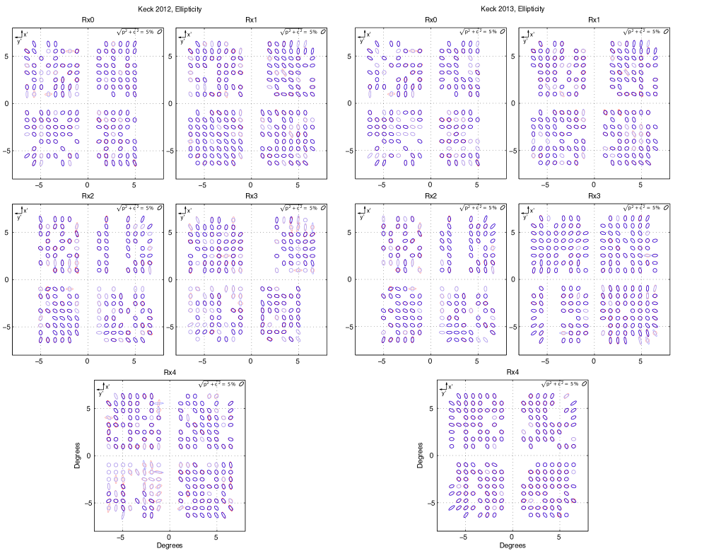
Figure 13.— Per-detector beam ellipticity for the Keck Array 2012 and 2013 configurations as projected onto the sky. The ellipticity for each detector has been exaggerated for visibility, as shown in the legend. $A$ and $B$ beams are shown in red and blue, respectively, and light colors show detectors that are not used in analysis. Detectors in Receivers 0, 2, and three of the four tiles on Receiver 1 are the same between 2012 and 2013, and the correlation between years for those receivers is evident.

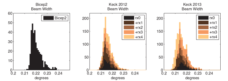
Figure 14.— Per-detector beam width ($\sigma$) measurements for Bicep2 (left-hand panel) and the Keck Array 2012 (middle panel) and 2013 (right-hand panel).

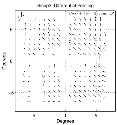
Figure 15.— The differential pointing measured between orthogonally polarized, co-located detector pairs, plotted in a focal plane layout for Bicep2. Arrows point from the $A$ detector location to the $B$ detector location, and the length of the arrows corresponds to the degree of mismatch multiplied by a factor of 20 for plotting. Detector pairs with grey arrows are not used in analysis.

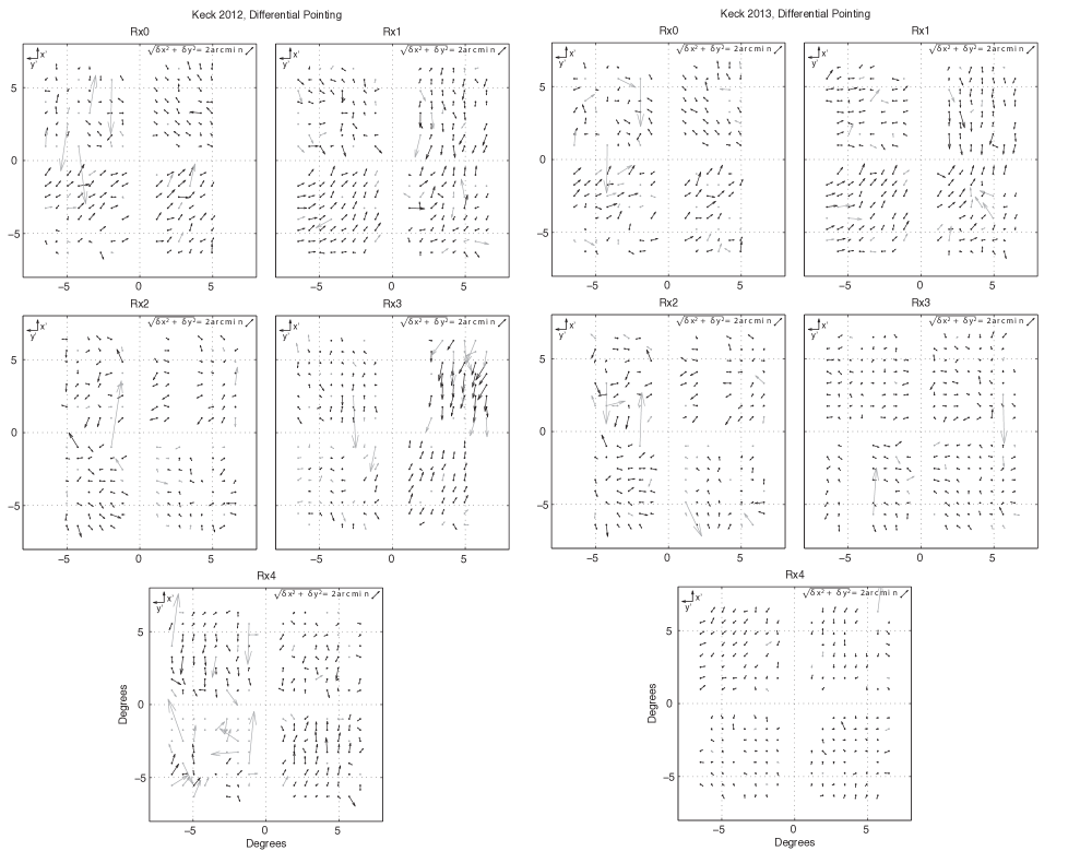
Figure 16.— The differential pointing measured between orthogonally polarized, co-located detector pairs, plotted in a focal plane layout for the Keck Array in its 2012 and 2013 configurations. Arrows point from the $A$ detector location to the $B$ detector location, and the length of the arrows corresponds to the degree of mismatch multiplied by a factor of 20 for plotting. Detector pairs with grey arrows are not used in analysis. Detectors in Receivers 0, 2, and three of the four tiles on Receiver 1 are the same between 2012 and 2013, and the correlation between years for those receivers is evident. Receiver 4 received a new focal plane in 2013 with reduced near-field differential pointing.

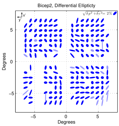
Figure 17.— The differential ellipticity measured between orthogonally polarized, co-located detector pairs, plotted in a focal plane layout for Bicep2. The major axes of the ellipses are proportional to $\sqrt{\delta p^{2}+\delta c^{2}}$, a measure of the magnitude of the differential ellipticity. A large fraction of detectors have beams whose ellipticity is well matched. Light colored detector pairs are not used in analysis. The differential ellipticity for each detector pair has been exaggerated for visibility, as shown in the legend.

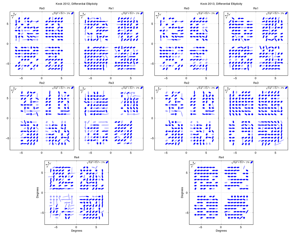
Figure 18.— The differential ellipticity measured between co-located detector pairs, plotted in a focal plane layout for the Keck Array 2012 and 2013. The major axes of the ellipses are proportional to $\sqrt{\delta p^{2}+\delta c^{2}}$, a measure of the magnitude of the differential ellipticity. Light colored detector pairs are not used in analysis. The differential ellipticity for each detector pair has been exaggerated for visibility, as shown in the legend. Detectors in Receivers 0, 2, and three of the four tiles on Receiver 1 are the same between 2012 and 2013, and the correlation between years for those receivers is evident.

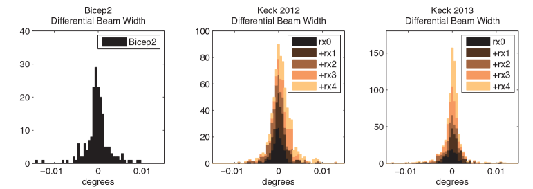
Figure 19.— The measured differential beam width between orthogonally polarized, co-located detector pairs for Bicep2 (left-hand panel) and the Keck Array 2012 (middle panel) and 2013 (right-hand panel).

3.2.2 Differential beam parameters

We calculate differential beam parameters for a pair of co-located orthogonally polarized detectors by taking the difference between the main beam parameters for each detector within the pair. The differential beam parameters are calculated for each beam map measurement. Receiver-averaged differential beam parameters for all detectors used in B-mode analysis are shown in Table 3. The uncertainties are calculated in the same way as in Table 2, described in Section 3.2.1. The scatter is dominated by true pair-to-pair differences, not measurement repeatability. The changes in the Keck Array beam parameters from 2012 to 2013 are explained by the focal plane reconfigurations described in Table 1.

Figures 15 and 16 show the measured differential pointing and Figures 17 and 18 show the measured differential ellipticity on a per-pair basis across the focal plane for Bicep2 and the Keck Array. Figure 19 shows histograms of the measured differential beam width on a per-pair basis for Bicep2 and the Keck Array.

We observe a pattern of far-field differential pointing across the focal plane (see Figures 15 and 16) that is different for each receiver and has no direct correlation with the observed near-field mismatch for a given focal plane, which also exhibits a pattern across the focal plane (see Section 3.1). The source of the far-field differential pointing could be an interaction of the observed near-field mismatch with possible imperfections in the optical system that would translate the near-field mismatch into the far field (see Section 3.1). The observed differential pointing per pair for Bicep2 was larger than that observed for Bicep1 and much larger than optical modeling of the telescope predicts (see Section 2).

The differential beam width for all receivers is small and does not have an observable pattern across the focal plane. While there is a large spread of per-detector ellipticities across the focal plane, ellipticities within each detector pair are relatively well matched, so the range of differential ellipticities for each detector pair is smaller than the scatter in the ellipticities on a per-detector basis. The differential ellipticities for Bicep2 and Keck Array are larger at the edges of each tile, evident in Figures 17 and 18.

Table 3Measured pair-difference beam parameters for Bicep2 and Keck Array receivers for 2012 and 2013

Receiver		Differential Beam Parameters
		Differential X Pointing	Differential Y Pointing	Differential Beam Width	Diff. Plus Ellipticity	Diff. Cross Ellipticity
		$dx_{i}$ (arcminutes)	$dy_{i}$ (arcminutes)	$d\sigma_{i}$ (degrees)	$dp_{i}$ ($+$)	$dc_{i}$ ($\times$)
Bicep 2		$0.81\pm 0.29\pm 0.14$	$0.78\pm 0.35\pm 0.14$	$0.000\pm 0.001\pm 0.001$	$-0.002\pm 0.013\pm 0.011$	$-0.003\pm 0.012\pm 0.005$
Keck 2012	Receiver 0	$0.60\pm 0.34\pm 0.07$	$-0.27\pm 0.63\pm 0.11$	$0.000\pm 0.001\pm 0.001$	$-0.011\pm 0.009\pm 0.003$	$-0.004\pm 0.008\pm 0.003$
	Receiver 1	$-0.025\pm 0.54\pm 0.09$	$-0.48\pm 0.45\pm 0.04$	$0.001\pm 0.002\pm 0.001$	$-0.007\pm 0.011\pm 0.002$	$-0.009\pm 0.006\pm 0.002$
	Receiver 2	$-0.25\pm 0.54\pm 0.09$	$0.14\pm 0.69\pm 0.09$	$-0.001\pm 0.002\pm 0.001$	$-0.007\pm 0.015\pm 0.002$	$-0.003\pm 0.009\pm 0.003$
	Receiver 3	$-0.39\pm 1.68\pm 0.06$	$-0.12\pm 0.35\pm 0.05$	$0.001\pm 0.002\pm 0.001$	$-0.007\pm 0.015\pm 0.002$	$-0.007\pm 0.008\pm 0.002$
	Receiver 4	$-0.04\pm 1.21\pm 0.08$	$-0.06\pm 0.33\pm 0.04$	$0.002\pm 0.002\pm 0.001$	$-0.002\pm 0.016\pm 0.003$	$-0.009\pm 0.009\pm 0.002$
Keck 2013	Receiver 0	$0.59\pm 0.39\pm 0.07$	$-0.26\pm 0.70\pm 0.06$	$0.000\pm 0.001\pm 0.001$	$-0.011\pm 0.009\pm 0.002$	$-0.004\pm 0.009\pm 0.002$
	Receiver 1	$0.03\pm 1.12\pm 0.06$	$-0.57\pm 0.56\pm 0.05$	$0.001\pm 0.002\pm 0.001$	$-0.010\pm 0.016\pm 0.002$	$-0.009\pm 0.006\pm 0.002$
	Receiver 2	$-0.26\pm 0.52\pm 0.12$	$0.10\pm 0.69\pm 0.11$	$-0.001\pm 0.002\pm 0.001$	$-0.007\pm 0.016\pm 0.003$	$-0.003\pm 0.009\pm 0.003$
	Receiver 3	$-0.09\pm 0.32\pm 0.12$	$-0.09\pm 0.47\pm 0.11$	$0.000\pm 0.001\pm 0.001$	$-0.001\pm 0.013\pm 0.004$	$-0.002\pm 0.009\pm 0.003$
	Receiver 4	$0.21\pm 0.46\pm 0.04$	$-0.14\pm 0.35\pm 0.02$	$0.000\pm 0.001\pm 0.001$	$-0.020\pm 0.005\pm 0.002$	$-0.002\pm 0.003\pm 0.001$

3.2.3 Comparison with optical models

Figure 20 shows a comparison between beams averaged over all pairs of detectors used in analysis Bicep2 and the results of the Zemax physical optics model discussed in Section 2.7. Also shown is a Gaussian fit to the beams. The cross section shown is taken along the scan direction, which is aligned with the horizon. The Zemax simulation is monochromatic, which gives rise to the sharp nulls in the Airy rings that are smoothed out in the real data due to the wider bandpass of the detectors. Otherwise, the agreement between the measured beams and simulation is good.

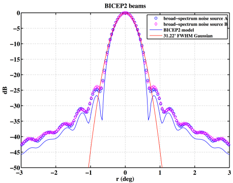
Figure 20.— Cross section of Bicep2 beams (averaged over all pairs of detectors used in analysis) compared with Zemax physical optics simulations and a Gaussian fit. The agreement between the measured beams and the simulation is good, and the data are well-fit by a Gaussian model near the peak.

3.3. Far sidelobes

Far sidelobes of the telescope can potentially see the bright Galactic plane, features on the ground, or emission from the Moon. The telescope ground shield systems for Bicep2 and the Keck Array were designed to mitigate contamination from the ground.

The ground shielding system, described in Takahashi et al. (2010) and in Section 2.6, has two main components. First, there is a co-moving absorptive forebaffle that rotates around the boresight with the telescope and intersects beams at $\sim 15^{\circ}$ from the peak. Second, there is a fixed reflecting ground shield. The additional loading on the detectors due to the forebaffle was measured to be $\sim$3–6 $\mathrm{K_{CMB}}$ in Bicep2 and $\sim$5–10 $\mathrm{K_{CMB}}$ in the Keck Array. The lowest loading was found for edge pixels and the highest loading was found for central pixels. This is higher than the measured Bicep1 value of $\sim$2 $\mathrm{K_{CMB}}$ (Takahashi et al., 2010). The origin of this coupling is attributed to a combination of scattering off the foam window, shallow-incidence reflections off the inner wall of the cold telescope tube, and residual out-of-band coupling. For the 2014 observing season, we implemented absorptive corrugations inside the telescope tube of each Keck Array receiver to reduce shallow-incidence reflections off the telescope tube. After the corrugations were installed, the total loading due to the forebaffle was reduced to 3 $\mathrm{K_{CMB}}$ for the 2014 observing season.

We measure the far-sidelobe response using a broad-spectrum noise source, described in Section 3.4.2, with fixed polarization. The source is mounted on a mast and sits $\sim 10$ m from the telescope so that the far sidelobes can be mapped with no flat mirror installed and with a very bright source. We achieve $\sim 70$ dB of dynamic range by performing the measurements at two different source brightnesses to achieve the signal-to-noise required to measure dim features far from the main beam while retaining the ability to measure the main beam itself without significant gain compression or instability.

In Bicep2, we observe that while there are no sharp features in the far-sidelobe regime (defined as having a geometry such that it could see Galactic emission during regular CMB observations), there is some power that is spread diffusely through the far-sidelobe region. Most of this power is intercepted by the forebaffle at $>15^{\circ}$ from the main beam. We integrate the total power in a typical beam profile to quantify the fraction of the power found outside of a given angle from the main beam center. We find that for a typical detector, less than 0.1% of the total integrated power is found outside of $25^{\circ}$ from the main beam for Bicep2 with the co-moving forebaffle installed. We have mapped the far sidelobes of the Keck Array and plan to perform a similar analysis.

To verify that the total power in the far sidelobes that intersects the forebaffle matches the amount of additional loading on the detectors due to the forebaffle, we make maps of the far-sidelobe response both with and without the forebaffle installed. We then measure the amount of far-sidelobe power that was intercepted by the forebaffle and compare it to the measured forebaffle loading on the detectors. For Bicep2, the fractional amount of power intercepted by the forebaffle averaged across the focal plane is 0.7%, corresponding to 3 $\mathrm{K_{CMB}}$ — consistent with the measured excess loading due to the forebaffle.

3.4. Polarization angle and cross-polar beam response

A key advantage of the Bicep2/Keck Array experimental approach is the ability to characterize the polarization angles, $\psi$, and cross-polar response, $\epsilon$, of each detector to high precision using ground-based calibrators. To calculate the cross-polar response, we first find the polarization angle that maximizes the total integrated amplitude of each detector’s response and then compare that amplitude with the amplitude when the radiation’s polarization is rotated by $90^{\circ}$ from that angle. This can be thought of as the monopole or gain term in the cross-polar response.

Precise characterization is made possible by Bicep2/Keck Array’s relatively short far-field range (beyond 70 m). Polarization angle calibration is important for constraining potential systematics. Large systematic uncertainty in the polarization orientation of the detectors with respect to the sky would lead directly to E-to-B leakage, resulting in false EB correlation. Because E and T are correlated, this would also result in false TB correlation.

The procedure we use to make polarization maps in our B-mode analysis only requires precise measurement of per-detector polarization angles, not of the overall rotation. We use correlations seen in the CMB itself via a self-calibration procedure using TB and EB correlations (Keating et al., 2013) to estimate the overall rotation angle. This CMB calibration procedure indicates a coherent rotation of $\sim 1^{\circ}$ for Bicep2, which is then removed in the B-mode analysis as described in the Systematics Paper.

We derive a benchmark for polarization angle measurement precision driven by systematics contamination requirements for a measurement of the BB spectrum that does not use the CMB self-calibration technique. Using the same technique presented in Takahashi et al. (2010) for Bicep1, we find a benchmark of $\Delta\psi<0.7^{\circ}$, corresponding to $r<0.01$. A more stringent benchmark of $\Delta\psi<0.2^{\circ}$ is required by the desire to measure the EB spectrum with high precision to test proposed cosmological mechanisms that generate a non-zero EB spectrum, such as cosmic birefringence (Carroll et al., 1990). The cross-polar response enters in analysis as a small adjustment to the overall polarization gain, but cannot create any false B-mode signal.

Bicep2 and the Keck Array use two different methods for determining polarization angles, which allows us to check for consistency between measurements and to look for systematics in the measurements themselves. The first method uses a thin rotating dielectric sheet placed directly above the vacuum window. The second method involves observing a rotating polarized source in the far field. In the following sections, we will discuss results from each method.

3.4.1 Dielectric sheet calibration

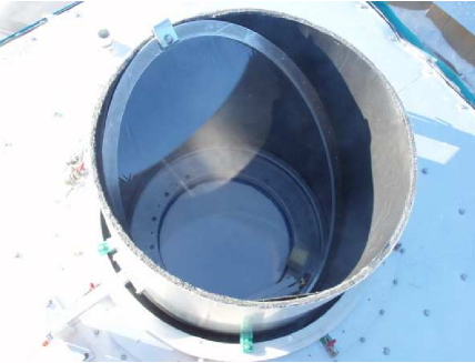
Figure 21.— A picture of the dielectric sheet calibrator installed on the Bicep1 telescope. We used this calibrator to measure the polarization angle and cross-polar response of Bicep2 as well.

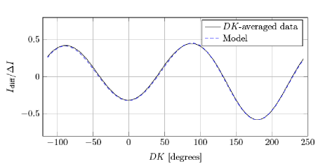
Figure 22.— The dielectric sheet calibrator pair-difference amplitude for a typical pair of detectors in Bicep2 ($I_{\mathrm{diff}}$), normalized by the difference in temperature between the warm absorber and the sky ($\Delta I$), plotted as a function of boresight rotation angle (DK). The fitted model is also plotted.

The dielectric sheet calibrator (DSC) is a thin plastic film oriented at a $45^{\circ}$ angle to the optical axis of the telescope, as shown in Figure 21. The telescope is free to rotate about its boresight with respect to the thin film. The film acts as a partially polarized beam splitter, preferentially reflecting one polarization of the beam into the warm absorptive lining around the splitter and transmitting the other polarization preferentially to the cold sky. The DSC is essentially a beam-filling polarized source with a brightness that scales with the difference in temperature between the sky and ambient. By rotating the telescope about its boresight and keeping the DSC fixed, we measure the polarization response of each detector as a function of boresight angle. This technique is fast and precise for relative angles, but is sensitive to the exact alignment of the calibrator with respect to the focal plane. An identical technique was used for Bicep1 (Takahashi et al., 2010).

To make measurements of the polarization angle, the DSC is installed in place of the forebaffle directly above the vacuum window of the telescope. Because a substantial fraction of the beam is transmitted to the sky, data are acquired only when the weather is good to avoid atmospheric noise in the measurement. A film thickness and index are chosen to provide the requisite signal-to-noise while avoiding gain instability in the detectors. The detectors are then biased onto either the titanium or aluminum superconducting transition. Before acquiring the calibration scan, the telescope is dipped in elevation to provide an unpolarized signal modulation from which a relative gain correction between $A$ and $B$ detectors is derived. Scans are acquired by counter-rotating in boresight rotation and azimuth with the telescope pointed at zenith. The counter-rotation fixes the beam location on the sky while the calibrator (attached to the azimuth axis but not the boresight rotation axis) rotates about the boresight of the telescope.

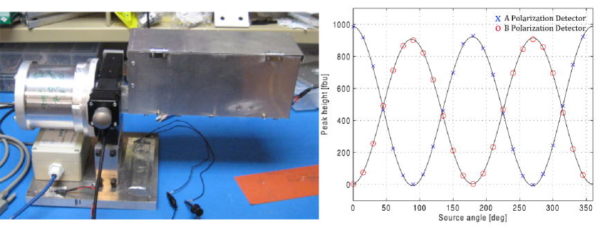
Figure 23.— Left: The rotating polarized amplified thermal broad-spectrum noise source used for polarization characterization. Right: Polarization modulation vs. source angle of an example detector pair from Bicep2, measured using the rotating polarized source.

An example of the periodic modulation of the detector pair-difference signal observed under rotation of the DSC for Bicep2 is shown in Figure 22. The geometric model that we use to extract the polarization angle for a given detector from the observed modulation (Takahashi et al., 2010) relies on a few externally measured quantities: the tilt of the dielectric sheet, the sheet material properties including the index of refraction and thickness, and the incident angle of each of the detectors on the film. The tilt of the sheet was measured with respect to gravity with a digital level before and after each scan and was close to $45^{\circ}$. The lateral tilt across the surface of the dielectric sheet was also measured with a digital level. Between installations of the calibrator, the value was observed to change by as much as $1.5^{\circ}$, but during a measurement it was repeatably measured to ¡$0.02^{\circ}$. The polarization angle is a weak function of both the index of refraction and the sheet thickness. The incident angles of the detectors are taken from detector centroid fits in the far field.

With these external inputs accurately measured, the model leaves only two free parameters. The first is the polarization angle $\psi$ of each detector. The second free parameter is the amplitude of the signal ($\Delta I$), which is proportional to the difference in temperature between the absorptive lining and the sky temperature at zenith and is a nuisance parameter. The amplitude, normalized by the brightness difference between the warm absorber and the sky, is extremely well-matched to the model of the polarized signal expected from the dielectric sheet.

For Bicep2, polarization angles are derived from a total of five independent measurements acquired between August 2010 and December 2012. The first three measurements used a 2 mil thick Mylar film and the final two measurements were taken with a thinner 1 mil sheet. To combine the results, weights are derived from the inverse variance of the residual after subtracting the fitted model. Using these measurements, the per-detector polarization angles have a statistical error of ¡$0.2^{\circ}$. In the Bicep2 B-mode analysis, we adopt the per-detector polarization angles from the DSC for use in making polarization maps.

We took first measurements with the DSC for Keck Array receivers after the 2013 observing season, and plan to follow up with more complete measurements in future seasons.

3.4.2 Rotating polarized source measurements

We also measure the polarization angle and the cross-polar response of each detector using a rotating polarized broad-spectrum noise source that we have developed for use with Bicep2 and the Keck Array, shown in Figure 23, and called the Rotating Polarized Source (RPS) (Bradford, 2012). The initial version of the broad-spectrum noise source emitted radiation in the 140–160 GHz range, designed to cover the passband of Bicep2 and the initial installation of Keck Array receivers. Subsequently, the source was retrofitted to cover the frequency bands of Keck Array receivers at 95 GHz and 220 GHz. A $50~{}\Omega$ load provides room-temperature thermal noise at the input of the first stage of amplification (80 dB). A series of frequency multipliers, amplifiers, and filters bring the output frequency to the desired range (140–160 GHz for use with 150 GHz receivers). Linearly polarized radiation is emitted by a 15 dBi horn antenna, and is further polarized by a free-standing wire grid, yielding cross-polar leakage of the source $<0.03$%. Two variable attenuators in series allow for control of output power over a large dynamic range, making the source useful for multiple applications, including polarization measurements, far-field beam mapping, and sidelobe mapping with the source closer to the receiver. A microwave switch chops the source at $\sim 18$ Hz. For RPS measurements, the entire source is mounted on a stepped rotating stage and has a total positional repeatability $<0.01^{\circ}$.

To map the response of every detector as a function of polarization angle incident on the detector, we set the polarized source to a given polarization angle and scan in azimuth over the source over a tight elevation range to obtain beam maps of one physical row of detectors on the focal plane at one polarization angle. We then repeat this measurement in steps of $15^{\circ}$ in source polarization angle over a full $360^{\circ}$ range. After completing all source polarizations for a given row of detectors, we move to the next row of detectors and repeat the sequence. We repeat the entire set of measurements at two distinct boresight rotation angles as a consistency check. An example of the polarization modulation as a function of source angle for one pair of Bicep2 detectors is shown in Figure 23.

We perform a five-parameter least squares fit to the detector response as a function of angle to extract a polarization angle and cross-polar response for each detector. The model is described as:

$$A\left(\cos{(2(\theta+\psi))}+\frac{1+\epsilon}{1-\epsilon}\right)\left(C\cos{(\theta+\phi)}+1\right),$$ (15)

where $\theta$ is the angle of the source, $\epsilon$ is the cross-polar response of each detector, $\psi$ is the polarization angle of each detector, $A$ is the amplitude of the source, and $C$ and $\phi$ are the amplitude and phase of a source collimation term, common across all detectors and describing any misalignment between the source rotation axis and the source alignment axis. The source collimation misalignment gives rise to a sinusoidal response with a period of $360^{\circ}$, while the polarization modulation has a period of $180^{\circ}$. This allows us to separate the two effects, since the parameters are not degenerate.

The cross-polar response is very low for detectors in Bicep2, typically $\sim 0.4$%, with less than 10% of detectors showing cross-polar response greater than 1%. This is consistent with the known level of crosstalk between two detectors in a given polarization pair and the level of direct island coupling in the detectors, discussed in the Instrument Paper and the Detector Paper.

3.4.3 Polarization beam characterization

In Section 3.4.2 we described our measurements of the monopole term in the cross-polar response and the polarization angle of each detector pair using the RPS. We can also use RPS measurements to investigate higher-order terms of the cross-polar response, which lead to E-to-B leakage. The higher-order response can be expressed by defining $T$, $Q$, and $U$ beams for each detector, which we call $B_{T}$, $B_{Q}$, and $B_{U}$. For a sky signal with linear polarization expressed in the detector $Q$/$U$ coordinate system, the full detector response is given by an integral of the $T$, $Q$, and $U$ beams over solid angle,

$$\int{\left[B_{T}(\mathbf{x})T(\mathbf{x})+B_{Q}(\mathbf{x})Q(\mathbf{x})+B_{U}(\mathbf{x})U(\mathbf{x})\right]d\Omega}.$$ (16)

To define the detector $Q$ and $U$ axes, we adopt the convention that the integral of $B_{U}$ is zero, i.e. $B_{U}$ has no monopole component. This choice decouples the description of $B_{Q}$ and $B_{U}$ from absolute calibration of the detector polarization angles. An alternate sensible choice, setting the $Q$ axis to the polarization angle of the $A$ or $B$ detector, produces similar results in practice.

The two detectors in an ideal orthogonally polarized pair would have the same $B_{T}$ as each other, the same $B_{Q}$ but with opposite sign from each other, and zero $B_{U}$. For that case, the sum of the two detectors in the pair (the “pair sum”) has response to $T$ only and the difference between the two detectors in the pair (the “pair difference”) has response only to $Q$. Imperfectly matched $B_{T}$ between detectors in a pair causes temperature to polarization leakage, which is covered extensively in Section 3.2.2 and the Systematics Paper. In this Section, we focus on $B_{Q}$ and $B_{U}$.

The $B_{T}$, $B_{Q}$, and $B_{U}$ for each detector are measured from RPS observations. We start with a set of beam maps for each detector, taken at 24 RPS grid angles spaced by $15^{\circ}$ steps. First, the maps are rescaled to correct for the collimation offset described in Section 3.4.2 and to achieve uniform relative calibration for paired detectors. Then, the 24 maps for each detector are summed with uniform weighting to form $T$ maps, $\cos 2\theta$ weighting to form $Q$ maps, and $\sin 2\theta$ weighting to form $U$ maps, where $\theta$ is equal to the angle between the RPS polarization axis and the detector $Q$ axis.

Figure 24 shows the measured $B_{T}$, $B_{Q}$, and $B_{U}$ for the pair sum and pair difference combinations of a single typical pixel in Bicep2. To reduce measurement noise, these maps have been smoothed with a $0.1\arcdeg$ Gaussian kernel. The pair difference $B_{T}$ (upper right panel) shows the differential pointing that is prominent in Bicep2. Structure in the pair sum $B_{Q}$ and $B_{U}$ causes polarization to temperature leakage, which is unimportant.

While the monopole response of the pair difference $B_{U}$ is zero by construction, there is some higher-order response to $U$, which can be seen in the bottom panels of Figure 24. We do not include these higher-order $B_{U}$ effects in the main power spectrum analysis; therefore, power in the pair difference $B_{U}$ could cause uncorrected polarization rotation that would lead to E-to-B leakage. The amplitude of the pair difference $B_{U}$ is typically $\lesssim 0.8\%$ of $B_{Q}$. In the power spectrum this amplitude is squared, so the effective EE-to-BB leakage is $\lesssim 6\times 10^{-5}$. The resulting contamination at $\ell\sim 90$–125 is $\sim 5\times 10^{-5}\mu\textrm{K}^{2}$. This is a factor of 10 below the $r=0.01$ BB signal, so this effect is negligible for Bicep2. Furthermore, boresight rotation and variation among detectors can provide additional cancellation of the E-to-B leakage, although we do not rely on such cancellation in the above argument.

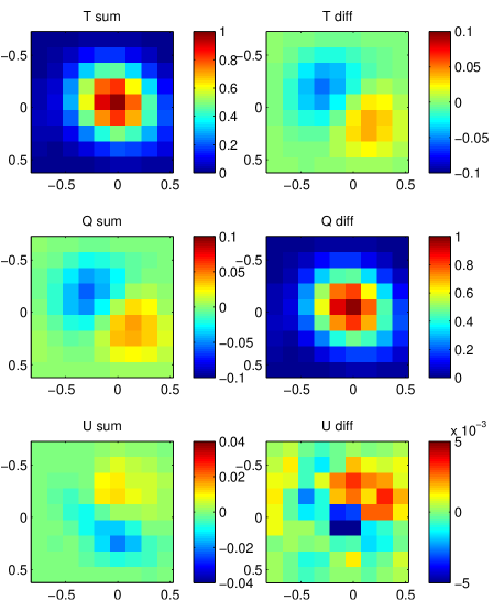
Figure 24.— The Stokes $T$, $Q$, and $U$ beam maps ($B_{T}$, $B_{Q}$, and $B_{U}$) for a single typical pixel in Bicep2 from RPS measurements, smoothed with a $0.1\arcdeg$ Gaussian kernel. The left column shows the response of the sum of the detectors in a pair; the right column shows the pair difference response. The pair difference $B_{T}$ and pair sum $B_{Q}$ both show the differential pointing present in Bicep2. An ideal instrument would have no $U$ response. Only the pair difference beams are relevant to Bicep2 polarization analysis. The small ($\lesssim 0.8\%$) features in the pair difference $B_{U}$ cause a negligible amount of E-to-B leakage. The larger feature in the pair sum $B_{U}$ beam would cause polarization to temperature leakage, which is harmless. Note that the color scales are not uniform across panels.

4. Simulation and deprojection of mismatched elliptical beams

The Bicep2 and Keck Array simulation pipeline is fully described in the Systematics Paper and the Results Paper. We give here a brief description, discussing the role of detailed beam map measurements in simulations.

The beam pattern of a single detector can be characterized as a set of perturbations on a circular Gaussian fit with a nominal width ($\sigma_{\mathrm{n}}$) equal to the receiver-averaged value and a nominal beam center equal to the calculated center for the pair of detectors from the initial elliptical Gaussian fit. We consider the first six perturbations, corresponding to the templates shown in Figure 25. These six templates correspond to relative responsivity, x-position offset, y-position offset, beam width, ellipticity in the “plus” orientation, and ellipticity in the “cross” orientation. To first and second order, these six perturbations of a circular Gaussian directly relate to the derivatives of the beam-convolved temperature sky, $T$, which we use to remove temperature to polarization leakage. The data processing pipeline is capable of removing leakage induced by beam mismatch modes that correspond to mismatch modes of elliptical Gaussian beams, and is described in the Systematics Paper. However, as shown in Figure 11, the beams are not perfectly described by an elliptical Gaussian. We take advantage of the detailed, high signal-to-noise beam maps described in Section 3.2 to fully describe the response of the detectors in the far field. To capture the effects of each detector’s beam on the science data and to understand any residual beam mismatch leakage after deprojection, we use the beam maps to run “beam map” simulations.

The beam map simulations can use an arbitrary two-dimensional convolution kernel for the beam of each detector, which is convolved with a flat projection of the 143 GHz Planck temperature map (Planck Collaboration, 2014a; Planck HFI Core Team, 2011) and interpolated to produce simulated detector timestreams. The simulated timestreams are then fed into the regular data processing pipeline, ensuring that the processing and filtering of the real data are applied to the simulated timestreams. The simulated timestreams are binned into maps and then deprojected with the same template that is used for real data. The flat-sky approximation in principle limits the accuracy of the simulation at a level of $r\sim 10^{-4}$, which in practice is lower than the observed leakage, discussed in the Systematics Paper.

Since we have high-quality, high signal-to-noise beam maps for nearly every detector used in the science analysis, we use these beam maps as two-dimensional convolution kernels in the beam map simulations, allowing us to study precisely the effects of the real beam on the science data for every detector. The results of the beam map simulations have been used in the Results Paper.

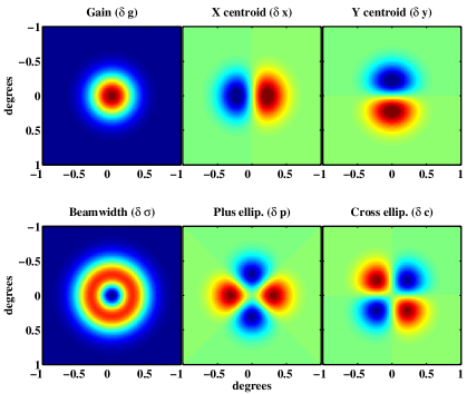
Figure 25.— Differential beam templates resulting in mismatch in (a) responsivity (b) x-position (c) y-position (d) beam width (e) ellipticity in plus orientation (f) ellipticity in cross orientation. In the limit of small differential parameters, a differenced beam pattern constructed from the difference of two elliptical Gaussians can be represented as a linear combination of each of these templates.

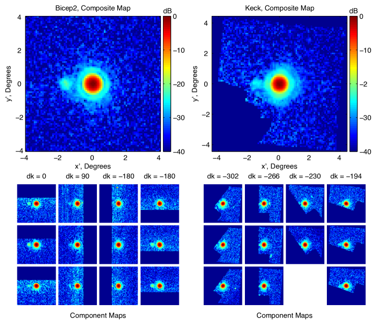
Figure 26.— Left: An example composite beam map for a Bicep2 detector using twelve beam maps. Right: An example composite beam map for a Keck Array detector using eleven beam maps. The maps are rotated to account for the boresight rotation angle and then added. The color scale is logarithmic with decades marked in dB.

4.1. Per-detector beam maps

The two-dimensional convolution kernels that are fed into the beam map simulation pipeline are constructed from a composite of the the far-field beam maps that we describe in Section 3.2. For Bicep2, we use beam maps taken with the 45 cm diameter thermal source. The maps were taken in November 2012, and the complete set consists of a total of twelve maps: three sets of maps taken at four boresight rotation angles separated by $90^{\circ}$. The three different sets of maps were taken using different aluminum transition bias points to find the optimal response for as many detectors as possible and to reduce gain compression artifacts that appeared in a small subset of detectors. The thermal source is only $\sim 2^{\circ}$ above the horizon, so we mask out the ground in these beam maps by masking the portion of the map that is $>1.5^{\circ}$ from the main beam and along the horizon. Even with a chopped source, the hot ground causes response in the detectors that is visible in the demodulated maps. We rotate the maps to account for the boresight angle, and the maps are then centered on the common beam centroid for each detector pair. To make the composite map that is used in simulations, we take the median amplitude for each pixel across all the component maps. The left-hand panel of Figure 26 shows an example of the composite beam map for a single detector that has been built from the set of twelve component maps for Bicep2.

Taking a median filter across all maps allows us to downweight spurious signals in the individual maps that are not repeatable across maps, allowing us to make clean, high signal-to-noise maps. We find that the level of the noise in the composite beam maps is low enough to show no effect in the beam map simulations. Due to masking and rotation, not all pixels in the composite beam map use the same number of input beam maps. For a radius of $<1.2^{\circ}$ from the beam center, all twelve component maps are included in the composite map, and all pixels use at least three beam maps.

The Keck Array composite beam maps for 2012 and 2013 are constructed from sets of maps taken in February 2012 and February 2013 respectively. The maps taken in February 2012 use the 20 cm diameter thermal source, and as a result have lower signal levels than the Bicep2 component maps and the Keck Array February 2013 maps, which use the 45 cm diameter thermal source. The Keck Array beam maps are constructed from a set of $\sim 25$ beam maps taken at ten different boresight rotation angles. For each receiver, we use beam maps taken at up to five boresight rotation angles where the receiver was positioned so that its beams reflect off of the large flat mirror and to the thermal source. The drum must be rotated so that a given receiver is physically near the bottom of the drum for the beams from that receiver to reflect off of the flat mirror and to the source. Therefore, only boresight rotation angles that place a given receiver near the bottom of the drum are used for composite maps for that receiver.

For each of the five boresight rotation angles for which detectors in a given receiver view the mirror, we cut maps for pixels that do not see the mirror. The number of maps that are included in each detector’s composite map for the Keck Array varies from a single map (for detectors at the edge of a focal plane on Receiver 0 for 2013) to a maximum of eleven component maps with a median of nine maps used per detector. In addition to masking the ground in Keck Array beam maps, we also mask the South Pole Telescope by masking out a rectangle that is $5^{\circ}$ wide and $2.5^{\circ}$ high, beginning $2.5^{\circ}$ to the left of the chopped thermal source as viewed by Keck Array receivers. We do not have beam maps for 9 detector pairs used in Keck Array analysis for 2012 and 28 detector pairs used in Keck Array analysis for 2013.

The right-hand panel of Figure 26 shows an example of the resulting composite beam map for a single detector for the Keck Array. As a result of the limited boresight rotation angle coverage, there is a portion of each map that is masked out in the composite map for each detector. We fill in the unmapped parts of the composite beam map by inserting the mean value from an azimuthal average around the beam center.

4.2. Simulation Results

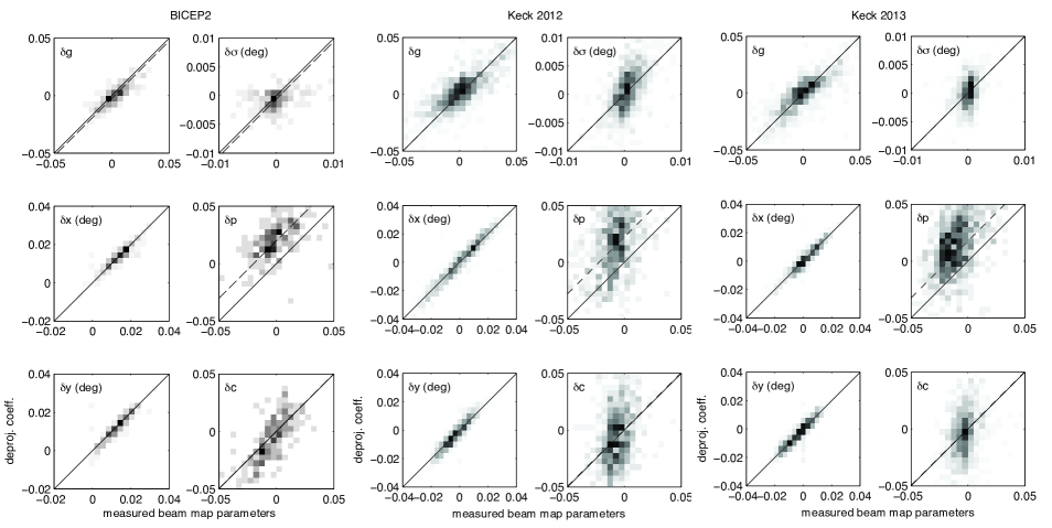
Figure 27.— A comparison of the deprojection coefficients recovered using our CMB observation data to the measured beam parameters for Bicep2 and the Keck Array 2012 and 2013. Measured differential gains for Bicep2 and the Keck Array are determined using the cross-correlation of T maps for individual detectors with Planck. The rest of the measured beam parameters are from beam maps. We observe a strong correlation for differential pointing and differential ellipticity for Bicep2, and a strong correlation for differential pointing in the Keck Array. The scatter for differential ellipticity for the Keck Array is higher than for Bicep2 because we have less data for the Keck Array compared to Bicep2 so the noise level is higher for the coefficients recovered from CMB observation data. The solid line indicates a one-to-one correlation. The bias in the recovered deprojection coefficients predicted by simulations is shown with the dashed line as an offset and is discussed in the Systematics Paper.

Comparing the beam map simulations with regular simulations, where beam mismatch modes are derived from CMB temperature data itself, we find that the beam map simulations accurately predict the leakage of the beam mismatch modes, discussed fully in the Systematics Paper. When we do not deproject any main beam mismatch modes, the contamination of the B-mode auto-spectrum is very well predicted by the beam map simulation. The beam map simulation spectra also predict the jackknife failures that we see in real data before deprojection.

Figure 27 compares the deprojection coefficients derived using CMB data to the measured beam parameters for Bicep2 and the Keck Array for the 2012 and 2013 configurations. Measured differential gains for Bicep2 and the Keck Array are determined using the cross-correlation of T maps for individual detectors with Planck. The rest of the measured beam parameters are from beam maps. The deprojection coefficients for Bicep2 show a correlation for all main beam mismatch modes, consistent with the observation that the measured beam parameters are the same main beam mismatch modes that are present in the real data. We also see a strong correlation for the differential pointing mismatch modes for the Keck Array. The Keck Array differential gain, beam width, and ellipticity modes show a large scatter in the recovered deprojection coefficients from real data compared to the measured beam parameters. This is because the deprojection coefficients for the Keck Array are obtained from one year of CMB data (since 2012 and 2013 must be calculated separately due to different receiver configurations), compared to three years for Bicep2, resulting in higher noise levels in the deprojection coefficients derived from real data.

4.3. Undeprojected residual mismatch

As described in the Systematics Paper, for the Bicep2 B-mode analysis presented in the Results Paper, we deproject differential pointing and gain and subtract the effects of differential ellipticity. These modes, however, do not fully describe the beams of Bicep2 and the Keck Array, which have small contributions from higher-order terms. Figure 11 shows an example detector and the residual power after removing an elliptical Gaussian fit, displaying the power contained in higher-order terms. The power in the per-pair difference beam that is not described by the six parameters in Figure 25 could be a source of temperature to polarization leakage.

Using beam map simulations, we can predict the amount of contamination in our BB spectrum from these additional (higher-order) beam mismatch modes that we do not deproject. Since the beam map simulations use the measured far-field response of each beam as inputs, they include the effect of all beam mismatch modes within $4^{\circ}$ of the beam center, limited only by the level of noise in the measurement of the far-field beams. Any effect from far sidelobes and residual power outside of $4^{\circ}$ from the beam center have been shown to be small (see Section 3.3).

After deprojecting differential pointing, gain, and ellipticity, the level of contamination predicted by beam map simulations is well below the sensitivity of Bicep2, as described in the Systematics Paper. For Bicep2, we have mitigated temperature to polarization leakage caused by per-pair beam mismatch to a level sufficient to detect $r\simeq 0.003$ (BICEP2 Collaboration, 2015). We have also limited the contribution from additional systematics to $r\lesssim 0.006$ (BICEP2 Collaboration, 2015).

5. Conclusions

We have fully described the optical system and characterized the optical performance of the Bicep2 experiment and the Keck Array 2012 and 2013 configurations. We have performed a full beam mapping campaign in situ at the South Pole and have measured far-field beam shape parameters, near-field beam shapes, detector polarization angles, per-pair cross-polar response, and far-sidelobe response.

We find that measured beam shapes match physical optics simulations well, but that for a given pair of orthogonally polarized detectors, there can be significant differences in beam shape in the far field, especially in differential pointing between the two detectors. We find that the level of E-mode to B-mode leakage is less than $r\simeq 0.001$ for Bicep2, and in the Systematics Paper we show that the remaining temperature to polarization leakage due to residual, higher-order components of the differential beam is at the level of $r\simeq 0.003$ for Bicep2, well below the sensitivity of the experiment. We expect the level of leakage due to beam effects to be similar for the Keck Array.

References

- Ade et al. (2006) Ade, P. A. R., Pisano, G., Tucker, C., & Weaver, S. 2006, in Society of Photo-Optical Instrumentation Engineers (SPIE) Conference Series, Vol. 6275, Society of Photo-Optical Instrumentation Engineers (SPIE) Conference Series
- Ahmed et al. (2014) Ahmed, Z., Amiri, M., Benton, S. J., et al. 2014, in Society of Photo-Optical Instrumentation Engineers (SPIE) Conference Series, Vol. 9153, Society of Photo-Optical Instrumentation Engineers (SPIE) Conference Series
- Aikin (2013) Aikin, R. W. 2013, PhD thesis, California Institude of Technology
- Aikin et al. (2010) Aikin, R. W., et al. 2010, Millimeter, Submillimeter, and Far-Infrared Detectors and Instrumentation for Astronomy V, 7741, 77410V
- BICEP2 Collaboration (2014a) BICEP2 Collaboration. 2014a, The Astrophysical Journal, 792, 62
- BICEP2 Collaboration (2014b) —. 2014b, Physical Review Letters, 112, 241101
- BICEP2 Collaboration (2015) —. 2015, arXiv:1502.00608
- BICEP2, Keck Array, and Spider Collaborations (2015) BICEP2, Keck Array, and Spider Collaborations. 2015, arXiv:1502:00619
- Bradford (2012) Bradford, K. J. 2012, Undergraduate thesis, Harvard University
- Carroll et al. (1990) Carroll, S. M., Field, G. B., & Jackiw, R. 1990, Phys. Rev. D, 41, 1231
- Filippini et al. (2010) Filippini, J. P., Ade, P. A. R., Amiri, M., et al. 2010, in Society of Photo-Optical Instrumentation Engineers (SPIE) Conference Series, Vol. 7741, Society of Photo-Optical Instrumentation Engineers (SPIE) Conference Series
- Hinderks et al. (2009) Hinderks, J. R., Ade, P., Bock, J., et al. 2009, Astrophys. J., 692, 1221
- Kamionkowski et al. (1997) Kamionkowski, M., Kosowsky, A., & Stebbins, A. 1997, Physical Review Letters, 78, 2058
- Keating et al. (2013) Keating, B. G., Shimon, M., & Yadav, A. P. S. 2013, Astrophys. J. Lett., 762, L23
- Keating et al. (2003) Keating, B. G., et al. 2003, Proc. SPIE Int. Soc. Opt. Eng., 4843, 284
- Lamb (1996) Lamb, J. W. 1996, International Journal of Infrared and Millimeter Waves, 17, 1997
- Leitch et al. (2002) Leitch, E. M., Pryke, C., Halverson, N. W., et al. 2002, Astrophys. J., 568, 28
- O’Brient et al. (2012) O’Brient, R., Ade, P. A. R., Ahmed, Z., et al. 2012, in Society of Photo-Optical Instrumentation Engineers (SPIE) Conference Series, Vol. 8452, Society of Photo-Optical Instrumentation Engineers (SPIE) Conference Series
- Ogburn IV et al. (2010) Ogburn IV, R. W., et al. 2010, Proceedings of the SPIE: Millimeter, Submillimeter, and Far-Infrared Detectors and Instrumentation for Astronomy V, 7741, 77411G
- Planck Collaboration (2014a) Planck Collaboration. 2014a, Astr. & Astroph., 571, A1
- Planck Collaboration (2014b) —. 2014b, Astr. & Astroph., 571, A22
- Planck HFI Core Team (2011) Planck HFI Core Team. 2011, Astr. & Astroph., 536, A6
- Runyan et al. (2003) Runyan, M. C., Ade, P. A. R., Bhatia, R. S., et al. 2003, Astrophys. J. Suppl., 149, 265
- Seljak (1997) Seljak, U. 1997, Astrophys. J., 482, 6
- Seljak & Zaldarriaga (1997) Seljak, U., & Zaldarriaga, M. 1997, Physical Review Letters, 78, 2054
- Sheehy et al. (2010) Sheehy, C. D., et al. 2010, Millimeter, Submillimeter, and Far-Infrared Detectors and Instrumentation for Astronomy V, 7741, 77411R
- Takahashi et al. (2010) Takahashi, Y. D., et al. 2010, Astrophys. J., 711, 1141
- Vieregg et al. (2012) Vieregg, A. G., et al. 2012, Proceedings of the SPIE: Millimeter and Submillimeter Detectors and Instrumentation for Astronomy VI, 8452
- Yoon et al. (2006) Yoon, K. W., et al. 2006, in Society of Photo-Optical Instrumentation Engineers (SPIE) Conference Series, Vol. 6275, Society of Photo-Optical Instrumentation Engineers (SPIE) Conference Series