Cold magnetized quark matter phase diagram within a generalized SU(2) NJL model

Abstract

We study the effect of intense magnetic fields on the phase diagram of cold, strongly interacting matter within an extended version of the Nambu-Jona-Lasinio model that includes flavor mixing effects and vector interactions. Different values of the relevant model parameters in acceptable ranges are considered. Charge neutrality and beta equilibrium effects, which are specially relevant to the study of compact stars, are also taken into account. In this case the behavior of leptons is discussed.

I Introduction

The influence of intense magnetic fields on the properties of strongly interacting matter has become an issue of increasing interest in recent years 1 . This is mostly motivated by the realization that in some relevant physical situations, like high energy non-central heavy ion collisions 2 and compact stellar objects called magnetars 3 , very strong magnetic fields may be produced. Since in these systems extreme temperatures and/or densities may be found, it is interesting to investigate which modifications are induced by the presence of strong magnetic fields on the whole QCD phase diagram. Unfortunately, even in the absence of those fields, the present knowledge of such phase diagram is only schematic due to the well-known difficulty given by the so-called sign problem which affects lattice calculations at finite chemical potential 5 . Of course, the presence of strong magnetic fields makes the situation even more complex. Thus, most of our present knowledge of their effect comes from investigations performed in the framework of effective models (see e.g. 6 and refs. therein). In this contribution we present some results of a study of the phase diagram of cold quark matter subject to intense magnetic fields in the framework of a generalized Nambu-Jona-Lasinio (NJL) model. The NJL-type models are effective relativistic quark models for non perturbative QCD, where gluon degrees of freedom are integrated out and interactions are modelled through point like interactions. In its simplest version njl it only includes scalar and pseudo scalar interactions that describe chiral symmetry breaking effectively. As well known, however, a more detailed description of the low-energy quark dynamics requires that other channels like flavor mixing and vector meson interactions are taken into account reports . In fact, some aspects of the effect of those interactions on the magnetized quark matter have already been investigated Boomsma:2009yk ; Denke:2013gha . The purpose of the present work is to extend those analyzes by performing a detailed study of the resulting cold matter phase diagrams, including their dependence on the parameters that regulate the strength of these interactions. Moreover, the behavior of cold magnetized quark matter under conditions relevant for the physics of compact stars will also be considered. One of the phenomena to be discussed in detail is that related to the so-called inverse magnetic catalysis (IMC) expected to exist at low temperature and moderate values of the chemical potentials  Preis:2010cq . It is important to mention that, despite bearing a similar name, this phenomenon is different from the inverse magnetic catalysis at finite temperature found in lattice QCD (LQCD). Concerning the latter one, we recall that most effective models foresee that at zero chemical potential a crossover transition is obtained at a pseudo critical temperature $T_{c}$ that increases with an increasing magnetic field, a behavior which is contrary to the one found in LQCD calculations Bruckmann:2013oba . In fact, recently there have been significant efforts to modify the models such that they incorporate a mechanism that could lead to inverse magnetic catalysis around $T_{c}$ (see Ref. Andersen:2014xxa for a recent review on this issue). We should stress, however, that this is not expected to affect the low temperature behavior discussed in this work.

This paper is organized as follows. In Sec. II we provide some details of the model and its parametrizations as well as the way to deal with an external constant magnetic field. In Sec. III we present and discuss our results for symmetric quark matter. The situation for stellar matter is analyzed in Sec. IV. Finally, our conclusions are given in Sec. V.

II Formalism

We consider a generalized NJL-type SU(2) Lagrangian density which includes a scalar-pseudoscalar interaction, vector-axial vector and the t´Hooft determinant interaction reports . In the presence of an external magnetic field and chemical potential it reads:

$$\mathcal{L}=\bar{\psi}\left(i\ \hbox to0.0pt{/\hss}\!D-m_{c}+\hat{\mu}\ \gamma^{0}\right)\psi+\mathcal{L}_{int}$$ (1)

where

$$\mathcal{L}_{int} = G_{1}\sum_{a=0}^{3}\left[\left(\bar{\psi}\tau_{a}\psi\right)^{2}+\left(\bar{\psi}i\gamma_{5}\tau_{a}\psi\right)^{2}\right]+G_{2}\sum_{a=0}^{3}\left[\left(\bar{\psi}\gamma_{\mu}\tau_{a}\psi\right)^{2}+\left(\bar{\psi}\gamma_{\mu}\gamma_{5}\tau_{a}\psi\right)^{2}\right]$$ (2)

$$+G_{3}\left[\left(\bar{\psi}\gamma_{\mu}\psi\right)^{2}+\left(\bar{\psi}\gamma_{\mu}\gamma_{5}\psi\right)^{2}\right]+G_{4}\left[\left(\bar{\psi}\gamma_{\mu}\psi\right)^{2}-\left(\bar{\psi}\gamma_{\mu}\gamma_{5}\psi\right)^{2}\right]+2G_{D}\left(d_{+}+d_{-}\right)$$

Here, $G_{i}$ with $i=1,4$ and $G_{D}$ are coupling constants, $\psi=\left(u,d\right)^{T}$ represents a quark field with two flavors, $d_{\pm}=det\left[\bar{\psi}\left(1\pm\gamma_{5}\right)\psi\right]$, $\hat{\mu}=\mathrm{diag}\left(\mu_{u},\mu_{d}\right)$ the quark chemical potentials, $m_{c}$ is the (current) mass matrix that we take to be the same for both flavors, $\tau_{0}=I$, where $I$ is the unit matrix in the two flavor space, and $\tau_{a}$, $0~{}<~{}a~{}\leq~{}3$ denote the Pauli matrices. The coupling of the quarks to the electromagnetic field ${\cal A}_{\mu}$ is implemented through the covariant derivative $D_{\mu}=\partial_{\mu}-i\hat{q}{\cal A}_{\mu}$ where $\hat{q}$ represents the quark electric charge matrix $\hat{q}=\mathrm{diag}\left(q_{u},q_{d}\right)$ where $q_{u}/2=-q_{d}=e/3$. In the present work we consider a static and constant magnetic field in the 3-direction, ${\cal A}_{\mu}=\delta_{\mu 2}x_{1}B$. In the mean-field approximation the associated grand-canonical thermodynamical potential for cold and dense quark matter reads

$$\Omega^{\mathrm{MFA}}=-\sum_{f=u,d}\theta_{f}+\Omega_{pot}$$ (3)

where $\theta_{f}$ gives the contribution from the gas of quasi-particles of each flavor $f=u,d$ and can be written as the sum of 3 contributions Menezes:2008qt

$$\theta^{\mathrm{vac}}_{f} = \frac{N_{c}}{8\pi^{2}}\ \left\{\Lambda\left(2\Lambda^{2}+M_{f}^{2}\right)\sqrt{\Lambda^{2}+M_{f}^{2}}-M_{f}^{4}\ln\left[\frac{(\Lambda+\sqrt{\Lambda^{2}+M_{f}^{2}})}{M_{f}}\right]\right\}\mbox{,}$$

$$\theta^{\mathrm{mag}}_{f} = \frac{N_{c}}{2\pi^{2}}\ (|q_{f}|B)^{2}\ \left[\zeta^{(1,0)}(-1,x_{f})-\frac{1}{2}(x_{f}^{2}-x_{f})\ln x_{f}+\frac{x_{f}^{2}}{4}\right]\mbox{,}$$

$$\theta^{\mathrm{med}}_{f} = \frac{N_{c}}{4\pi^{2}}\ |q_{f}|B\ \sum_{\nu=0}^{\nu^{max}_{f}}\alpha_{\nu}\left[\tilde{\mu}_{f}\sqrt{\tilde{\mu}_{f}^{2}-s_{f}(\nu,B)^{2}}\right.$$ (4)

$$\left.\qquad\qquad\qquad-s_{f}(\nu,B)^{2}\ln\left(\frac{\tilde{\mu}_{f}+\sqrt{\tilde{\mu}_{f}^{2}-s_{f}(\nu,B)^{2}}}{s_{f}(\nu,B)}\right)\right]\mbox{,}$$

where $M_{f}=m_{c}+\sigma_{f}$ and $\tilde{\mu}_{f}=\mu_{f}-\omega_{f}$, with $\sigma_{f}$ and $\omega_{f}$ being the mean field values of the scalar and vector meson fields, respectively. $\Lambda$ represents a non covariant ultraviolet cutoff and $\zeta^{(1,0)}(-1,x_{f})=d\zeta(z,x_{f})/dz|_{z=-1}$ where $\zeta(z,x_{f})$ is the Riemann-Hurwitz zeta function. In addition, $s_{f}(\nu,B)=\sqrt{M_{f}^{2}+2|q_{f}|B\nu}$ while $x_{f}=M_{f}^{2}/(2|q_{f}|B)$. In $\theta^{med}_{f}$, the sum is over the Landau levels (LL´s), represented by $\nu$, while $\alpha_{\nu}=2-\delta_{\nu 0}$ is a degeneracy factor and $\nu^{max}_{f}$ is the largest integer that satisfies $\nu^{max}_{f}\leq(\tilde{\mu}_{f}^{2}-M^{2}_{f})/(2|q_{f}|B)$.

The $\Omega_{pot}$ contribution reads

$$\Omega_{pot}=\frac{(1-c_{s})(\sigma_{u}^{2}+\sigma_{d}^{2})-2c_{s}\,\sigma_{u}\,\sigma_{d}}{8g_{s}(1-2c_{s})}-\frac{(1-2c_{v})(\omega_{u}^{2}+\omega_{d}^{2})+c_{v}\,\omega_{u}\,\omega_{d}}{8g_{v}(1-2c_{v})}$$ (5)

where we have introduced a convenient parametrization of the coupling constants in terms of the quantities $g_{s}$, $c_{s}$, $g_{v}$ and $c_{v}$ given by

$$g_{s}=G_{1}+G_{D}\qquad;\qquad g_{v}=G_{2}+G_{3}+G_{4}$$

$$c_{s}=\frac{G_{D}}{G_{1}+G_{D}}\qquad;\qquad c_{v}=\frac{G_{3}+G_{4}}{2(G_{2}+G_{3}+G_{4})}$$ (6)

The relevant gap equations are given by

$$\frac{\partial\Omega^{\mathrm{MFA}}(\sigma_{u},\sigma_{d},\omega_{u},\omega_{d})}{\partial(\sigma_{u},\sigma_{d},\omega_{u},\omega_{d})}=0\ .$$ (7)

The solutions to the gap equations minimize the thermodynamic potential with respect to the quark masses $M_{f}$, but the $\omega_{f}$ derivatives amount to a consistency condition and the potential is actually a maximum with respect to these variables. Several solutions will generally exist, corresponding to different possible phases, and the most stable solution is that which minimizes the thermodynamic potential with respect to $M_{f}$.

In our calculations we will consider first the simpler case of symmetric matter where both quarks carry the same chemical potential $\mu$. Afterwards, we will analyze the case of stellar matter in which leptons are also present and $\beta$-equilibrium and charge neutrality are imposed. In this case the chemical potential for each quark, $\mu_{f}$, is a function of quark number chemical potential $\mu$ and the lepton chemical potentials which have to be self-consistently determined.

In order to analyze the dependence of the results on the model parameters, we will consider two SU(2) NJL model parameterizations. Set 1 corresponds to that leading to $M_{0}=340$ MeV while Set 2 to that leading to $M_{0}=400$ MeV. Here, $M_{0}$ represents the vacuum quark effective mass in the absence of external magnetic fields. The corresponding model parameters are listed in Table 1.

Table 1: Parameter sets for the NJL SU(2) model.

Parameter set	$M_{0}$	$m$	$g_{s}\Lambda^{2}$	$\Lambda$	$-<u\bar{u}>^{1/3}$
	MeV	MeV		MeV	MeV
Set 1	340	5.595	2.212	620.9	244.3
Set 2	400	5.833	2.440	587.9	240.9

The presence of the t’Hooft determinant interaction is very important since it reflects the $U_{A}(1)-$anomaly of QCD. Its strength, and consequently the amount of flavor mixing induced by this term, is controlled by the parameter $c_{s}$. An estimate for its value can be obtained from the $\eta-\eta^{\prime}$ mass splitting within the $3-$flavor NJL model Kunihiro:1989my . This leads to $c_{s}\simeq 0.2$ Frank:2003ve . In any case, to obtain a full understanding of the effects of flavor mixing we will vary the value of $c_{s}$ in a range going from $0$, which corresponds to a situation in which the two flavors are completely decoupled, to $0.5$, being this the case of maximum flavor mixing described for example in Ref. Allen:2013lda . Regarding the vector coupling term it is important to recall that one can obtain naturally the terms proportional to $G_{2}$ if one starts from a QCD-inspired color current-current interaction and then performs a Fierz transform into color-singlet channels, and that in this case the relation between coupling strengths is $G_{2}=G_{1}/2$ reports . Yet, the value of $g_{v}$ cannot be accurately determined from experiments nor from lattice QCD simulations and this is why it has been taken as a free parameter in most works. In the present work we take $0<g_{v}/g_{s}<0.5$. It is worth mentioning that due to the mixing of pseudoscalar and longitudinal axial vector interaction terms, pseudoscalar meson properties depend on $G_{2}$. Thus, strictly speaking the parameters given in Table 1 only lead to the empirical values of $f_{\pi}$ and $m_{\pi}$ when $G_{2}=0$. However, as shown in Ref. Hanauske:2001nc , $m_{\pi}$ and $f_{\pi}$ only change by $\sim 10\%$ when $G_{2}/G_{1}$ increases from $0$ to $1$. Thus, for simplicity, we will keep the model parameter values fixed when varying $g_{v}$. A last comment regarding $c_{v}$, i.e. the parameter that regulates the ratio between the singlet and octet vector-axial vector interaction strengths: we will take it as a free parameter in the range $0\leq c_{v}\leq 1/2$. Note that for $c_{v}=1/2$ only singlet vector-axial interactions are present and, thus, there is no mixing between the pseudoscalar and longitudinal axial vector channels.

We end this section by describing the way in which the different phases of the magnetized quark matter will be denoted as well as the procedure used to identify the boundaries between them. For the phases we adopt the notation of Refs. Allen:2013lda ; ebert . Thus, the vacuum (i.e. fully chirally broken) phase is denoted by B, the massive phases in which $M_{f}$ depends on the chemical potential by $\mbox{C}_{\alpha}$ and, finally, the chirally restored phases by $\mbox{A}_{\alpha}$. Here, $\alpha$ is a set of two numbers indicating the highest LL populated for each flavor. To obtain the critical chemical potentials at a given $eB$ we proceed as follows. In the case of first order phase transitions we calculate the thermodynamical potential for each of the neighboring phases (that is, the global minimum with respect to $M_{f}$) and then search for the chemical potential values at which they become degenerate. In the case of crossover transitions the critical value is identified by the peak of the chiral susceptibility corresponding to each quark flavor, defined as $\partial{<\overline{\psi}\psi>}/\partial{m_{f}}$.

III Results for Symmetric matter

In this section we present the results obtained for the case of symmetric matter. These results were obtained solving the set of coupled “gap equations” (14) for different values of magnetic field and chemical potential.

III.1 Effect of the flavor mixing interactions

To neglect vector interactions implies taking $G_{2}=G_{3}=G_{4}=0$ in Eq. (2), while $G_{1}\neq 0$ and $G_{D}\neq 0$. Therefore, Eqs. (7), will become a set of two coupled equations that must be solved for the independent variables $M_{u}$ and $M_{d}$. The parameter $c_{s}$ acts as a coupling between both flavors and we study how the phase transitions are modified as we vary this parameter in the range $0<c_{s}<0.5$. The case $c_{s}=0.5$ corresponds to ordinary NJL where flavor mixing is maximum and, thus, both flavors have identical behavior. In fact, the first term in Eq. (5) will tend to infinity as $c_{s}$ goes to $0.5$ unless $M_{u}=M_{d}$, which leaves only one equation to be solved. But if $c_{s}<0.5$, then both masses will be independent variables, and transitions for each flavor might occur simultaneously or not in different regions of the phase diagrams.

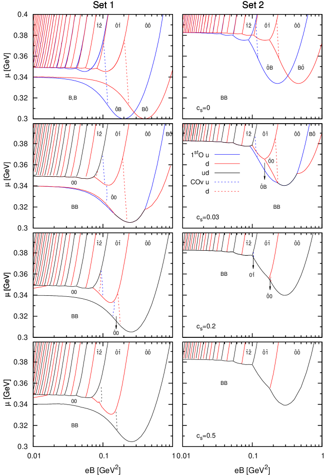
Figure 1: (Color online) Phase diagrams in the $eB-\mu$ plane for different values of flavor-mixing parameter $c_{s}$. To simplify the figure we have introduced a compact notation to indicate the phases. The pair of integers $mn$ corresponds to the $\mbox{C}_{mn}$ phase and the pair ${\bar{m}}{\bar{n}}$ to the $\mbox{A}_{mn}$ phase. The case in which one quark is in a C-type phase and the other in the A-type phase is indicated by putting a bar on top of the integer associated with the A-type phase.

The phase diagrams for both parameter sets and several values of flavor mixing can be seen in Fig. 1. We will start by commenting some general features which are common to all phase diagrams discussed in this work. It is seen that chiral symmetry is completely broken for chemical potentials well below $M_{0}$ and that restoration occurs for high enough chemical potentials, usually accompanied by a large drop in the dressed mass. The inclusion of a constant magnetic field modifies the quark dispersion relation, introducing Landau levels (LL’s) into its spectrum. A consequence of this is that chiral symmetry restoration might occur in several steps as chemical potential is increased, each of which is a transition where quark population appears on previously unoccupied LL’s. The restored chiral symmetry region consists of several phases with different number of LL’s occupied, which are separated by the so-called Van Alphen De Haas transitions, whose form is in the absence of vector mesons approximately $\mu_{c}=\sqrt{2k|q_{f}|B}$ (being this condition exact for the chiral case). As a result of the different quark electric charges, one up transitions is found every two down transitions when a phase diagram is traversed in the magnetic field direction at high enough fixed $\mu$. In all phase diagrams, a “main transition” is found, which separates the vacuum phase from the phases with populated LL’s and at fixed $eB$ it is the one with the lowest possible chemical potential (e.g.: lower black line in bottom left diagram in Fig. 1). In some cases, another main transition within the populated phase exists. It connects phases with partially restored symmetry and low LL population to the fully restored symmetry phases, where the Van-Alphen De Haas transitions are present and LL level population may be much higher. All of this gives rise to a potentially complex phase diagram, whose precise form depends on the parameter set and magnetic field (The $B=0$ case is simple yet depending on the parameter set there can be a few differences). The lower main transition usually shows, for moderate magnetic fields, a decrease of $\mu_{c}$ when $eB$ increases that is sometimes called magnetic anticatalysis Preis:2010cq (even though the name is more generally used to refer to the decrease of the quark condensates as $eB$ increases). For higher values of the magnetic field this tendency is reverted, and this gives rise to a characteristic curve in the main transition line to which we will refer as the “IMC well”. It is also worth noting that some of the other transitions in the phase diagrams also exhibit an IMC-like behavior.

Now we will discuss how the phase diagrams are modified as the parameter $c_{s}$ is varied. The upper two panels correspond to the $c_{s}=0$ case (no flavor mixing), which was previously studied in Ref. Allen:2013lda . In a sense, each flavor will have its own independent phase diagram because the gap equations are decoupled. Here, each line corresponds to a transition where LL population of a single quark flavor occurs (red lines for down quarks, blue lines for up quarks). Both flavors will coincide for $eB=0$ where SU(2) symmetry is recovered and behave differently as $eB$ increases, due to their different electric charges. Since this is the only difference between the equations for both flavors and since it only appears in the product $q_{f}B$, the down flavor phase diagram may be obtained from the other one through the replacement $q_{u}B=(2q_{d})B=q_{d}(2B)$ which amounts to a stretching of the up flavor phase diagram along the $eB$ axis. In other words, since the down quark has a smaller coupling to the field than the up quark, it will require a magnetic field twice as large to replicate the effect on an up quark. As a consequence of this, the IMC wells are shifted with respect to each other, so there will be a large well-distinguished region where up quarks exist in the lowest LL (LLL) while down quarks are in vacuum (0B), and another region where the opposite occurs (B0).

For finite $c_{s}$ (second row onwards in Fig. 1), the coupling between flavors creates a complex pattern, where transitions move closer together to the point of coalescing in some regions, that is, the LL population changes simultaneously for both flavors (these are represented by black lines). We can see that already for $c_{s}=0.03$, the transitions in both parameter sets occur together for low magnetic fields, and then separate for $eB=0.02$ GeV² in Set 1 and $eB=0.1$ GeV² in Set 2. Note that for $c_{s}=0$, the transitions for both flavors cross around $eB=0.12$ GeV² (for both sets). When flavor mixing is introduced, this crossing point transforms into a line, that is, both transitions occur together once again in an interval of magnetic field values. When $c_{s}=0.03$, they separate at $eB=0.4$ GeV², which is intuitive since a higher magnetic field will further break SU(2) flavor symmetry. For $c_{s}=0.2$ this separation is no longer seen in the diagrams but it can be guessed that it does occur beyond $eB=1$ GeV², and that for any value of $c_{s}<0.5$ there will always be a large enough magnetic field that will cause the $u$ and $d$ main transitions to separate.

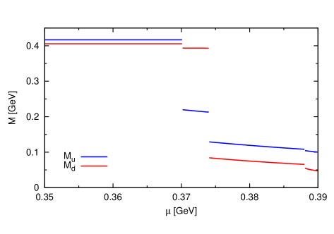
Figure 2: (Color online) Dressed masses for both flavors for Set 2, $c_{s}=0.03$, for $eB=0.11$ GeV².

For a better understanding of the physical meaning of the transition lines, we present in Fig. 2 the dressed masses for both flavors for Set 2, $c_{s}=0.03$, for $eB=0.11$ GeV². When the first discontinuity is encountered, at $\mu=370$ MeV, $M_{u}$ jumps to half its value and its LLL becomes populated. On the other hand, the down flavor remains in vacuum. Actually, its mass presents a small discontinuity caused by the weak coupling to the up quark which is not to be interpreted as a down transition. The down quark LLL is occupied at $\mu=374$ MeV. This is precisely the kind of behavior that generates a rich phase diagram for low $c_{s}$ values. The difference in masses is understood in terms of the effect of magnetic catalysis. Since the flavors have different charges, they couple with different intensities to the magnetic field, so the up quark will have a larger mass in the vacuum phase and a lower one in the populated phases, which is consistent with the fact that mass increases with magnetic field in the vacuum phase and decreases in the populated phase.

The behavior of the crossovers as $c_{s}$ is varied from $0$ to $0.5$ is interesting to note. For $c_{s}=0$, in Set 1, there is one crossover for each flavor. When $c_{s}$ is increased, the up crossover is slightly shifted to the left when crossing from the $00$ to the $01$ phase, acquiring a small discontinuity. In turn, a down crossover starts to appear from the left in the latter phase. As $c_{s}$ is increased, these two crossovers move towards each other, while the up crossover in $00$ shifts to the right, also moving towards the down crossover originally existing in that same phase. The $c_{s}=0.5$ limit, in which down and up crossovers have joined, is achieved very slowly, being the crossovers still separated for $c_{s}\simeq 0.4995$.

The first order transitions for both flavors already occur together in the whole studied region for $c_{s}=0.2$, so the qualitative behavior is very similar to the full flavor mixing case $c_{s}=0.5$. In fact, the model tends to full mixing quite quickly and only for $c_{s}<0.1$ are relevant mixture effects (or more precisely, the absence of it) actually seen. VA-dH lines are brought together for a particularly small amount of mixing, already coinciding for $c_{s}=0.03$, while crossover transitions, on the other hand, tend much more slowly to the $c_{s}=0.5$ behavior.

III.2 Effect of the vector interactions

In this section we analyze the effect of vector interaction terms. As discussed in the previous section, for $c_{s}\gtrsim 0.1$ the phase diagrams do not present qualitative variations. Here, therefore, we consider $c_{s}=0.2$ which also is in the range of realistic values suggested in Ref. Frank:2003ve . Although the results to be shown below correspond to $c_{v}=0$, our studies show that only small quantitative differences occur when varying this parameter from $0$ to $1/2$.

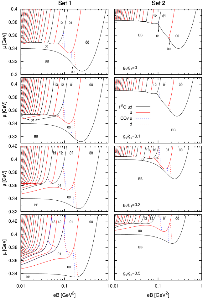
Figure 3: (Color Online) Phase diagrams in the $eB-\mu$ plane for different values of $g_{v}/g_{s}$. Different phases are denoted as in Fig. 1

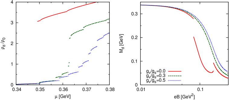
Figure 4: (Color online) Quark density over nuclear matter density as function of the chemical potential for $eB=0.016$ GeV² (left) and current mass as function of magnetic field for $\mu=0.345$ GeV (right) for different values of $g_{v}/g_{s}$. Results correspond to $d$ flavor and were obtained with parameter Set 1.

In Fig. 3 we present a series of phase diagrams obtained for different values of the ratio $g_{v}/g_{s}$. For Set 1 we observe that as $g_{v}/g_{s}$ increases the two main transitions separate and several new transitions appear in between, in the low $eB$ region of the diagram. These are partially restored symmetry regions, where quark mass acquires an intermediate value. For Set 2 there is a unique main transition for $g_{v}=0$, but already for $g_{v}/g_{s}\simeq 0.1$ it will split into two, leaving a $00$ phase in between which was not present before. For larger values of $g_{v}/g_{s}$ the behavior is similar to that of Set 1. The existence of new transitions at low $eB$ as $g_{v}/g_{s}$ increases can also be appreciated in the left panel of Fig. 4, where we show $d$ quark density normalized to nuclear matter density ($\rho_{0}=0.17$ $fm^{-3}$) as a function of chemical potential for $eB=0.016$ GeV in Set 1. In the absence of vector interaction, the density jumps from close to $0$ to $3$ times nuclear matter density, while quark population jumps from $00$ to a phase where several LL’s are occupied. As $g_{v}$ increases, the amount of transitions increases too. In fact, increasing the vector interaction coupling has the same effect as going to a parameter set that reproduces a lower value of current mass $M_{0}$, described in Ref. Allen:2013lda . Notice that the phase diagram for Set 2 and $g_{v}/g_{s}=0.3$ is in this sense very similar to Set 1 and $g_{v}/g_{s}=0$.

It is interesting to analyze the effect of the vector interactions on the so-called inverse magnetic catalysis (IMC) mentioned in the Introduction. We recall that the IMC is usually related to a decrease of the critical chemical potential at intermediate values of the magnetic fields, a phenomenon that can be clearly observed in all the phase diagrams plotted in Figs. 1 and 3. However, while from Fig. 1 we see that the variation of the strength of flavor mixing interactions has basically no effect on the IMC effect, the situation is different for the vector interactions. In fact, from Fig. 3 we note that if we measure the depth of the IMC well as the difference in $\mu$ between the lowest critical chemical potential at vanishing magnetic field and the lowest possible one in the whole diagram, we find that this difference is reduced by an $84\%$ for Set 1 and by a $67\%$ for Set 2 when going from $g_{v}=0$ to $g_{v}/g_{s}=0.5$. To explain this feature we recall that the IMC effect can be understood in terms of the extra cost in free energy to form a fermion-antifermion condensate at finite $\mu$, $\Omega_{ext}$ Preis:2010cq . In the absence of vector interactions this extra cost basically originates in the LLL contribution to the medium term. Considering the chiral limit for simplicity, this contribution can be shown to be proportional to $B\mu^{2}$ for symmetric matter, and it tends to decrease the difference in free energy between the vacuum phase and the finite density phase. As it is clear from Eqs. (4, 5) the presence of the vector interactions introduces some modifications in $\Omega_{ext}$. In the case of the medium term, they imply the replacement $\mu_{f}\rightarrow\tilde{\mu}_{f}=\mu_{f}-\omega_{f}$. Moreover, there is a new contribution coming from $\Omega_{pot}$. Thus, assuming as above that there is LLL dominance and that quarks are massless in the chirally restored phase, the extra cost for symmetric matter is

$$\Omega_{ext}=\frac{N_{c}B}{4\pi^{2}}\sum_{f}|q_{f}|(\mu-\omega)^{2}+\frac{\omega^{2}}{4g_{v}}$$ (8)

where, for simplicity, we have assumed $c_{v}=1/2$. The generalization for arbitrary values of $c_{v}$ is straightforward and, in addition, the numerical dependence on $c_{v}$ of the estimates to be given below turns out to be negligible. Of course, $\omega$ should satisfy the associated gap equation which follows from Eq. (14) in the Appendix. Within the above mentioned approximations, the solution of this equation is

$$\omega=\left[1+\frac{\pi^{2}}{N_{c}g_{v}\sum_{f}|q_{f}|B}\right]^{-1}\mu$$ (9)

Replacing in Eq. (8) we get that $\Omega_{ext}$ can be expressed in a form similar to that obtained in the absence of vector interactions, but where $\mu$ has to multiplied by a factor $1/\sqrt{1+N_{c}g_{v}eB/\pi^{2}}$. Note that the actual values of the $u-$ and $d-$quark charge have been already used to obtain this factor. Thus, in the region $eB\sim 0.2$ GeV² around which this expression is approximately valid we expect

$$\frac{\mu_{c}(g_{v})}{\mu_{c}(0)}\simeq\sqrt{1+\frac{N_{c}}{\pi^{2}}\ eB\ g_{v}}$$ (10)

For example, for Set 2 we obtain that the lowest critical chemical potential (which occurs at about $eB=0.24$ GeV²) increases by about 10 % when going from $g_{v}=0$ to $g_{v}/g_{s}=0.5$. Together with the fact that the lowest $\mu_{c}$ at vanishing magnetic field stays basically constant for values of $g_{v}/g_{s}\gtrsim 0.1$ this explains the strong reduction of the IMC well.

Another aspect of the reduction of the IMC phenomenon induced by the presence of the vector interactions can be observed in the right panel of Fig. 4. There, we plot the current quark mass for $d$ quarks as a function of the magnetic field for Set 1, $\mu=345$ MeV and several $g_{v}/g_{s}$ values, where the system is in the $00$ phase at $eB=0$. As discussed in Ref. Allen:2013lda in this case an actual decrease of the mass as $eB$ increases is expected to exist. As we see, however, such a decrease is slower for larger values of $g_{v}$. It should be noticed that discontinuities appearing for $g_{v}/g_{s}=0$ corresponds to the $d$ quark transition from the phase $00$ to $\bar{0}\bar{1}$ and back.

IV Results for stellar matter

We now turn our attention to stellar matter, that is, matter where $\beta$-equilibrium and charge neutrality are imposed. In this case, electrons and muons are introduced into the system so that the thermodynamical potential receives an extra contribution Menezes:2008qt

$$\Omega^{lep} = \sum_{l=e,\mu}\sum_{\nu=0}^{\nu^{max}_{l}}\frac{|q_{l}|B\ \alpha_{\nu}}{4\pi^{2}}\left[\mu_{l}\sqrt{\mu^{2}-s_{l}(\nu,B)^{2}}-s_{l}(\nu,B)^{2}\ln\left(\frac{\mu_{l}+\sqrt{\mu_{l}^{2}-s_{l}(\nu,B)^{2}}}{s_{l}(\nu,B)}\right)\right]$$ (11)

where $\nu^{max}_{l}=\mbox{Int}[(\mu_{l}^{2}-m^{2}_{l})/(2|q_{l}|B)]$ and $s_{l}(\nu,B)=\sqrt{m_{l}^{2}+2|q_{l}|B\nu}$. We take $m_{e}=0.511$ MeV and $m_{\mu}=105.66$ MeV.

The $\beta$-equilibrium and charge neutrality conditions read

$$\mu_{d}=\mu_{u}+\mu_{e}\qquad,\qquad\mu_{e}=\mu_{\mu}$$ (12)

and

$$\rho_{e}+\rho_{\mu}=\frac{1}{3}\left(2\rho_{u}-\rho_{d}\right)\ ,$$ (13)

respectively. The lepton densities appearing in the last equation can be easily obtained from the derivatives of the total thermodynamical potential with respect to the corresponding chemical potentials.

Following the discussions in the previous section only results for $c_{s}=0.2$ will be presented. If charge neutrality is imposed on our system, there will be a fixed relation between the densities of the up and down quarks, which will be necessarily different unless they are both zero. So, even though the value of $c_{s}=0.2$ was close enough to the full mixing case according to what was established in previous sections, charge neutrality will cause the flavors to behave differently among themselves.

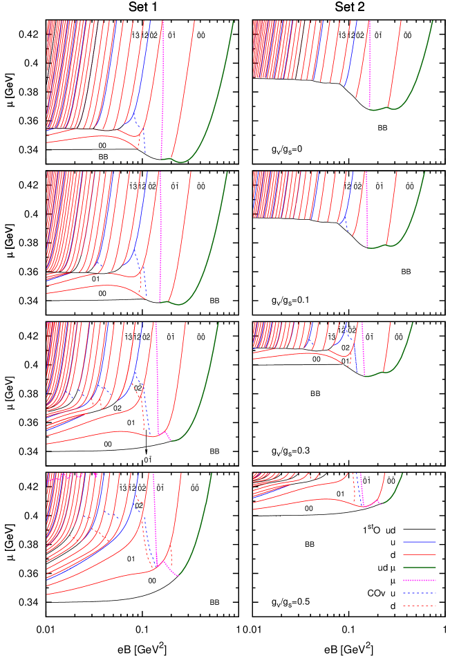
Figure 5: (Color online) Phase diagrams in the $eB-\mu$ plane for stellar matter and different values of $g_{v}/g_{s}$. Different phases are denoted as in Fig. 1. The pink dotted line represents muon transition from vacuum to LLL.

The phase diagrams in the $\mu-B$ plane for both parameter sets and for increasing values of $g_{v}$ are plotted in Fig. 5. The chemical potential $\mu$ on the horizontal axis is now the quark number chemical potential, in terms of which the flavor chemical potentials read $\mu_{f}=\mu-q_{f}\mu_{e}$ when Eqs.(12) are used. The introduction of stellar matter conditions has a few effects similar to those of vector interaction, in the sense that diagrams become similar to the ones corresponding to lower $M_{0}$ sets: main transitions separate for low $eB$ and several transitions appear in the region between them. The magnetic anticatalysis effect is reduced also: The depth of the anticatalysis well, as defined in the previous section, is reduced from $35$ MeV to $9$ MeV in Set 1 and from $43$ MeV to $22$ MeV in Set 2. As discussed in Ref. Grunfeld:2014qfa this can be understood by generalizing to stellar matter the discussion given in Sec.IIIb. We see that again the minimum critical chemical potential occurs at $eB\sim 0.2$ GeV². Around that value, and in the absence of vector interactions, the extra cost in free energy to form a fermion-antifermion pair at finite $\mu$ is in this case proportional to $B\bar{\mu}^{2}$ with $\bar{\mu}^{2}=\sum_{f}|q_{f}|\mu^{2}_{f}+\mu^{2}_{e}/3$. Here, a generally small muonic contribution has been neglected. Using the relations obtained from the $\beta$ equilibrium conditions, $\mu_{f}=\mu-q_{f}\mu_{e}$, we get $\bar{\mu}=\mu(1-2x/3+2x^{2}/3)^{1/2}$, where $x=\mu_{e}/\mu$. Note that the minus sign in the (dominant) linear term follows from the fact that $|q_{u}|=2|q_{d}|$. The relevant value of $x$ follows from the neutrality condition Eq. (13). Assuming as before that in the chirally restored phase we are dealing with massless quarks one obtains $x\simeq 0.38$ for $\mu\simeq 350$ MeV. Using this result we get $\bar{\mu}\simeq 0.92\ \mu$. This implies that the extra cost in free energy is smaller than that required in the symmetric matter case for the same value of $eB$ and $\mu$. Consequently, for a given $eB$, one needs a larger value of the chemical potential to induce the phase transition. In fact, we have $\mu_{c}^{st}/\mu_{c}^{sym}\simeq 1.09$ a value which is in good agreement with our full numerical results. In principle to determine the change in the IMC well we should also estimate the modification of $\mu_{c}$ at $eB=0$. As shown in Ref. Grunfeld:2014qfa this value also increases when stellar conditions are imposed. However, such an increase is several times smaller than the one at $eB\sim 0.2$ GeV² leading to a quenching of the IMC effect. As discussed in Sec.IIIb, the introduction of vector interaction will further enhance these effects. Consequently we observe that anticatalysis has completely disappeared for $g_{v}=0.5$.

The VA-dH transitions for different flavors also acquire relatively independent behaviors when charge neutrality is introduced. In particular, some down and up transitions occur simultaneously as we follow them upwards along the phase diagram and then separate visibly at a given chemical potential. This is most clearly seen at intermediate $eB\,(\simeq 0.1$ GeV²) for the transitions separating the $02$, $12$ and $13$ phases. The relationship for critical chemical potentials $\mu_{c}=\sqrt{2k|q_{f}|B}$, which occurred for symmetric matter now holds for each flavor chemical potential separately, where these two are different between themselves and related through Eq. (12). As a result of this, we see that in Fig. 5, which is instead plotted in terms of quark chemical potential, we roughly have one up transition every four down transitions, whereas in symmetric matter there was one up transition every two down transitions. In particular, for high $g_{v}$, the transitions have a tendency to clump up in groups of three (two down transitions and one up) with an intermediate down transition which is well separated from this group.

The transitions corresponding to the population of lepton Landau Levels are also included in Fig. 5. In all cases, it was seen that electron’s transition from vacuum to LLL occurs in the lower main transition, that is, quarks and electrons occupy their LLL simultaneously. This is understandable in that electrons have a very small, almost negligible mass, hence they will populate their LLL as soon as the associated chemical potential becomes finite. On the other hand, muon behavior is more complex. Since they have a larger mass than electrons it is expected that they will require a larger chemical potential to acquire a finite population. This is what actually happens in all our diagrams for low magnetic fields, where values larger than $430$ MeV are needed for this, hence not appearing in the plotted region. However, at intermediate values magnetic field values ($0.1<eB<0.2$ GeV²), this transition drops suddenly until it joins the lower main transition of the quarks. This happens because $\mu_{e}$ increases with magnetic field, allowing for muon population at lower quark chemical potential. For higher $eB$ values, all leptons and quark transitions occur together. The occupation of the first Landau Level of either lepton species requires much higher chemical potentials. This happens because leptons have a larger charge than quarks, leading to Landau Levels with larger energy, and because $\mu_{e}$ is only a slowly increasing function of $\mu$. The value needed for the first electron LL to be occupied, which is around $250$ MeV, is therefore only achieved near $\mu=900$ MeV. In some phase diagrams, the muon transition is seen to affect the behavior of the crossovers. This occurs because the $\mu_{e}$ is coupled to the order parameters, so a muon transition, with its corresponding jump in $\mu_{e}$, will affect the values of the quark masses and its associated susceptibilities. For $g_{v}/g_{s}=0.5$ in Set 1, for example, the down crossover separating the $00$ and $\bar{0}\bar{0}$ phases is smeared out near the muon transition. In other diagrams, like the one for $g_{v}/g_{s}=0.3$, the muon transition has completely absorbed the quark crossover.

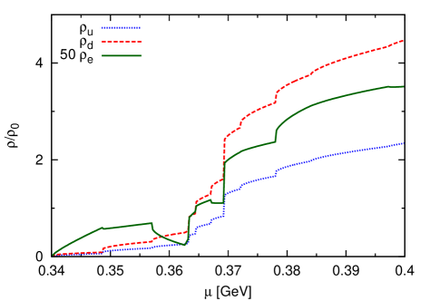
Figure 6: (Color online) Quark and electronic densities over nuclear matter density as functions of the chemical potential for $eB=0.02$ GeV². Results were obtained with $g_{v}/g_{s}=0.3$ and parameter Set 1.

In Fig. 6 we plot the normalized lepton densities together with those of the quarks as functions of the quark number chemical potential, for $eB=0.02$ GeV², $g_{v}/g_{s}=0.3$ and parameters of Set 1. All three densities become non zero simultaneously at $\mu=340$ MeV, where they all occupy their corresponding LLL. However, while quark density grows monotonously after the first transition, it is seen that when the next quark transition is encountered $\rho_{e}$ decreases, and jumps to an even lower value in the transition that follows. Recalling that these correspond to transitions of $d$ quarks and that the charge neutrality condition imposed is $\rho_{e}+\rho_{\mu}=(2\rho_{u}-\rho_{d})/3$, it can be understood that the electron density decreases whenever there is a $d$-transition and subsequent growth of $\rho_{d}$ (recall that $\rho_{\mu}=0$ in this range of chemical potential), without relevant changes in $\rho_{u}$. This is the case of this range of chemical potential and this value of magnetic field.

In Fig. 7 we show quark and lepton densities as functions of the magnetic field for $\mu=0.36$ GeV, for different strengths of the vector coupling. Results correspond again to Set 1. At low magnetic field, discontinuities in the quark densities, associated with the VA-dH transitions, are always encountered. For the cases with $g_{v}=0$ and $0.3$ a region is found in which $\rho_{d}$ changes its monotony within a C-type phase. This is because quarks can be found in this phase for magnetic fields high enough so the mass has started to increase with $eB$, and is associated to the region of the phase diagram above the IMC well. This behavior is not observed for $g_{v}/g_{s}=0.5$ where the IMC effect has disappeared. For $eB\sim 0.2$ GeV², $d$ quarks are already in a phase with a low $k$ and $u$ quarks with $k=0$, all densities increase and it is interesting to notice how slopes change whenever a $d$ transition is encountered. When $d$ quarks finally reach the $0$ phase all densities increase until they drop to zero when the last transition to vacuum is encountered.

V Conclusions

We have investigated how the phase diagram of cold strongly interacting matter is modified in the presence of intense magnetic fields in the context of NJL-type models which include flavor mixing and vector interaction. The whole range of possible flavor mixing values was swept through, going from the situation in which the two flavors are completely decoupled, to the one in which they are fully mixed. For low mixing values, a complex phase diagram is generated, but already for $c_{s}\simeq 0.1$, phase diagrams display a behavior that is qualitatively very similar to the full mixing case. Since SU(3) estimates suggest a value of $c_{s}\simeq 0.2$, it can be concluded that the realistic flavor mixing range is similar in behavior to the full mixing case. In what followed, vector interactions and stellar matter conditions were introduced. The most notable effect observed is that they attenuate the Inverse Magnetic Catalysis phenomenon, to the point that it completely disappears when both effects are jointly taken into account. It was also found that introducing vector interaction causes the two main transitions to separate and additional phases to appear between these two, effects that are similar to those occurring when changing to a parameter set that fits to a smaller dressed mass. In the stellar matter case, the behavior of the leptons was also studied. It was found that while electron LLL becomes populated simultaneously with quarks, the muon transition presents a more complicated dependence with the magnetic field. Namely, muon LLL requires a very high chemical potential to become populated at low $eB$, however, it joins the main quark transition together with electrons for high enough magnetic field.

APPENDIX

The explicit form of the gap equations is

$$\phi_{u}+\frac{(1-c_{s})\sigma_{u}-c_{s}\sigma_{d}}{4g_{s}(1-2c_{s})}=0\qquad;\qquad\rho_{u}-\frac{(1-2c_{v})\omega_{u}-c_{v}\omega_{d}}{4g_{v}(1-2c_{v})}=0$$

$$\phi_{d}+\frac{(1-c_{s})\sigma_{d}-c_{s}\sigma_{u}}{4g_{s}(1-2c_{s})}=0\qquad;\qquad\rho_{d}-\frac{(1-2c_{v})\omega_{d}-c_{v}\omega_{u}}{4g_{v}(1-2c_{v})}=0$$ (14)

where $\rho_{f}$ in the quark density for each flavor

$$\rho_{f}=\frac{N_{c}}{2\pi^{2}}|q_{f}|B\sum_{\nu=0}^{\nu^{max}_{f}}\alpha_{\nu}\sqrt{\tilde{\mu}_{f}^{2}-s_{f}(\nu,B)^{2}}$$ (15)

and $\phi_{f}$ can be written as the sum of three terms

$$\phi_{f}^{\mathrm{vac}} = -\frac{N_{c}M_{f}}{2\pi^{2}}\left[\Lambda\sqrt{\Lambda^{2}+M_{f}^{2}}-{M_{f}^{2}}\ln\left(\frac{\Lambda+\sqrt{\Lambda^{2}+M_{f}^{2}}}{{M_{f}}}\right)\right]\mbox{,}$$

$$\phi_{f}^{\mathrm{mag}} = -\frac{N_{c}M_{f}|q_{f}|B}{2\pi^{2}}\left[\ln\Gamma(x_{f})-\frac{1}{2}\ln(2\pi)\right.+\left.x_{f}-\frac{1}{2}\left(2x_{f}-1\right)\ln(x_{f})\right]\mbox{,}$$

$$\phi_{f}^{\mathrm{med}} = -\frac{N_{c}}{2\pi^{2}}\ M_{f}\ |q_{f}|B\sum_{\nu=0}^{\nu^{max}_{f}}\alpha_{\nu}\ \ln\left[\frac{\tilde{\mu}_{f}+\sqrt{\tilde{\mu}_{f}^{2}-s_{f}(\nu,B)^{2}}}{s_{f}(\nu,B)}\right]\mbox{,}$$ (16)

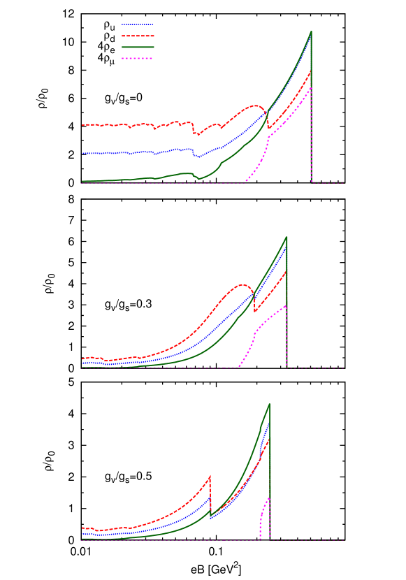
Figure 7: (Color online) Quark and lepton densities over nuclear matter density as function of the magnetic field for $\mu=0.36$ GeV for different values of $g_{v}/g_{s}$. Results were obtained with parameter Set 1.

References

- (1) D.E. Kharzeev, K. Landsteiner, A. Schmitt and H.-U. Yee, Lect. Notes Phys. 871 (2013) 1.
- (2) D.E. Kharzeev, L.D. McLerran and H.J. Warringa, Nucl. Phys. A803 (2008) 227.
- (3) R.C. Duncan and C. Thompson, Astrophys J. 392 (1992) L9.
- (4) F. Karsch, E. Laermann, 2004 Quark Gluon Plasma 3, edited by R.C.Hwa et al. (World Scientific Singapore), p.1.
- (5) E.S. Fraga, Lect. Notes Phys. 871 (2013) 121; R. Gatto and M. Ruggieri, Lect. Notes Phys. 871 (2013) 87.
- (6) Y. Nambu and G. Jona-Lasinio, Phys. Rev. 122 (1961) 345; 124 (1961) 246.
- (7) U. Vogl and W. Weise, Prog. Part. Nucl. Phys. 27 (1991) 195; S. Klevansky, Rev. Mod. Phys. 64 (1992) 649; T. Hatsuda and T. Kunihiro, Phys. Rep. 247 221 (1994) 221.
- (8) J. K. Boomsma and D. Boer, Phys. Rev. D 81 (2010) 074005.
- (9) R. Z. Denke and M. B. Pinto, Phys. Rev. D 88 (2013) 056008; D. P. Menezes, M. B. Pinto, L. B. Castro, P. Costa and C. Providência, Phys. Rev. C 89 (2014) 055207.
- (10) F. Preis, A. Rebhan and A. Schmitt, JHEP 1103 (2011) 033; F. Preis, A. Rebhan and A. Schmitt, Lect. Notes Phys. 871 (2013) 51.
- (11) F. Bruckmann, G. Endrodi and T. G. Kovacs, JHEP 1304 (2013) 112.
- (12) J. O. Andersen, W. R. Naylor and A. Tranberg, arXiv:1411.7176 [hep-ph].
- (13) D.P. Menezes, M.B. Pinto, S.S. Avancini, A. Pérez Martínez and C. Providência, Phys. Rev. C 79 (2009) 035807; D.P. Menezes, M.B. Pinto, S.S. Avancini and C. Providência, Phys. Rev. C 80 (2009) 065805; S.S. Avancini, D.P. Menezes and C. Providência, Phys. Rev. C 83 (2011) 065805.
- (14) T. Kunihiro, Phys. Lett. B 219 (1989) 363 [Erratum-ibid. B 245 (1990) 687].
- (15) M. Frank, M. Buballa and M. Oertel, Phys. Lett. B 562 (2003) 221.
- (16) P. G. Allen and N. N. Scoccola, Phys. Rev. D 88 (2013) 094005.
- (17) M. Hanauske, L. M. Satarov, I. N. Mishustin, H. Stoecker and W. Greiner, Phys. Rev. D 64 (2001) 043005.
- (18) D. Ebert, K. G. Klimenko, M. A. Vdovichenko, and A. S. Vshivtsev, Phys. Rev. D 61 (1999) 025005.
- (19) A. G. Grunfeld, D. P. Menezes, M. B. Pinto and N. N. Scoccola, Phys. Rev. D 90, 044024 (2014) [arXiv:1402.4731 [hep-ph]].