Fluctuation theorem between non-equilibrium states in an $RC$ circuit

Abstract

Fluctuation theorems impose constraints on the probability of observing negative entropy production in small systems driven out of equilibrium. The range of validity of fluctuation theorems has been extensively tested for transitions between equilibrium and non equilibrium stationary states, but not between general non equilibrium states. Here we report an experimental verification of the detailed fluctuation theorem for the total amount of entropy produced in the isothermal transition between two non-equilibrium states. The experimental setup is a parallel $RC$ circuit driven by an alternating current. We investigate the statistics of the heat released, of the variation of the entropy of the system, and of the entropy produced for processes of different durations. We show that the fluctuation theorem is satisfied with high accuracy for current drivings at different frequencies and different amplitudes.

1 Introduction

As already noted by Szilard in 1925 [1], entropy reduction can occur in a single realization of a thermodynamic process at the mesoscopic scale and the second law of thermodynamics is recovered when averaging over many realizations of such a process. At scales where thermal fluctuations are relevant, entropy-reducing trajectories can be observed [2, 3]. The fluctuations of the entropy production are governed by the so-called fluctuation theorems, which relate the probability to observe a trajectory destroying a certain amount of entropy to the probability to observe a trajectory producing the same amount of entropy [4, 5, 6, 7, 8, 9, 10, 11, 12, 13, 14]. In particular, they ensure that on average, the entropy production is positive. The fluctuation theorems are the building blocks of the emerging theory of stochastic thermodynamics, which describes the equilibrium and non-equilibrium thermodynamics of small systems, at the ensemble level as well as at the trajectory level [10, 15, 16, 17, 18, 19, 20, 21, 22, 23]. In parallel to the theoretical development of stochastic thermodynamics, the fluctuation theorems and the thermodynamics of small systems has been intensively investigated experimentally in last decade [2, 3, 24, 25, 26, 27, 28, 29, 30, 31, 32].

The fluctuation theorem for the total entropy production relates the probability $P(\Delta S_{\rm tot})$ to observe a trajectory producing an amount $\Delta S_{\rm tot}$ of entropy in a given thermodynamic process to the probability $\tilde{P}(-\Delta S_{\rm tot})$ to observe a trajectory destroying the very same amount of entropy in the time reversed or backward process, where the driving of the system is reversed in time [8, 11, 13, 14]:

$$\frac{P(\Delta S_{\rm tot})}{\tilde{P}(-\Delta S_{\rm tot})}=\exp\left(\frac{\Delta S_{\rm tot}}{k_{\rm B}}\right).$$ (1)

Equation (1) has a wide range of validity: It is valid for systems in contact with one or many heat baths, for transitions between stationary or non-stationary states or for systems in non-equilibrium stationary states. This fluctuation theorem has been experimentally tested for the transition between equilibrium states [33, 3], where it reduces to Crooks’ relation [7], for non-equilibrium steady-states [27, 29], and in the transition between non-equilibrium steady-states [25], where it can be refined to give the Hatano-Sasa relation [9]. More recently, the fluctuation theorem (1) was observed in a more general experiment involving a periodically driven system in contact with two heat baths at different temperatures [31]. All the aforementioned experiments have this in common, that at the end of the backward process, the system is in the same macroscopic state as at the beginning of the forward process.

In this paper, we report an experimental verification of the fluctuation theorem (1) in a situation where this is not case: In our experiment, the final state of the backward process is in general different from the state the system was prepared in at the beginning of the forward process. In such a transition, the fluctuation theorem (1) presents a subtlety, as realized by Spinney and Ford [14]. In fact, in general, the distribution $\tilde{P}$ appearing in the denominator in the left hand side of equation (1) is not the probability distribution of the entropy produced in the backward process. In general, $\tilde{P}$ is the distribution of a quantity which we will call conjugated entropy production in the following. However, in situations were the final state of the backward process is the same as the initial state of the forward process, conjugated entropy production and entropy produced in the backward process are equal. Hence, in those cases, $\tilde{P}$ is the probability distribution of the entropy produced in the backward process.

Our experimental system is a parallel $RC$ circuit driven by an alternative current. We verify the fluctuation theorem (1) for processes of arbitrary durations for different driving frequencies and intensities. Furthermore, we show the difference between conjugated entropy production and entropy produced in the backward process.

The paper is organized as follows. We begin by sketching the derivation of the fluctuation theorem (1) in section 2. In the derivation, we insist on the difference between the conjugated entropy production and entropy produced in the backward process. We continue by describing the experimental setup and protocol in section 3. In particular, we show how we sample forward and backward trajectories making the transition between two non-equilibrium states. Finally, we present our experimental results in section 4. We study the statistics of the heat dissipated to the environment, of the entropy produced and of the conjugated entropy production for different driving times. Furthermore, we show that the fluctuation theorem (1) is satisfied for different driving speeds and amplitudes. We close the paper with a short discussion of our results in section 5.

2 Detailed fluctuation theorem for the transition between two non-equilibrium states

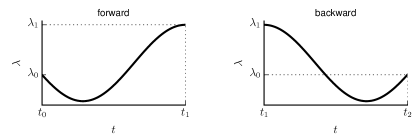
Figure 1: Forward (left panel) and time reverse (right panel) protocols.

We now sketch the derivation of equation (1) for the transition between two non-equilibrium states. Consider a small system in contact with a heat bath at temperature $T$, that can be driven by varying a control parameter $\lambda$. Initially, the value of the control parameter is set to $\lambda(t_{0})=\lambda_{0}$ and the system is prepared in a non-equilibrium macroscopic state $\rho(q,t_{0})=\rho_{0}(q)$. In other words, at time $t_{0}$, the probability that the mesoscopic state of the system is $q$ is given by the non-equilibrium distribution $\rho(q,t_{0})$. Due to the presence of thermal fluctuations, the mesoscopic state of the system cannot be controlled, but only the probability distribution of mesoscopic states. From time $t_{0}$ to $t_{1}$, the control parameter is changed from $\lambda(t_{0})=\lambda_{0}$ to $\lambda(t_{1})=\lambda_{1}$ according to a prescribed protocol $\lambda(t)$. The final macroscopic state of the system is $\rho(q,t_{1})=\rho_{1}(q)$. In the backward process, the initial state of the system is the final state of the forward process, $\rho_{1}(q)$, and the control parameter takes the same values as in the forward case but runs them backwards in time. Hence, we assume that the time reverse process starts just after the forward process ends, at time $t=t_{1}$. The control parameter is then varied according to $\lambda(t_{1}+t)=\lambda(t_{1}-t)$, as sketched in figure 1. The backward process ends at time $t_{2}=t_{1}+\tau$ where $\tau=t_{1}-t_{0}$ is the duration of both the forward and time reverse process. The final macroscopic state of the system is $\rho(q,t_{2})=\rho_{2}(q)$ which is in general different from $\rho_{0}(q)$.

The amount of entropy produced by a trajectory ${\bf m}=\{q_{t}:t_{0}\leq t\leq t_{1}\}$ in the forward process is given by [34, 35, 36, 13]:

$$\Delta S_{\rm tot}[{\bf m}]=k_{\rm B}\log\frac{{\mathcal{P}}_{\rm F}[{\bf m}]}{{\mathcal{P}}_{\rm B}[\bar{\bf m}]},$$ (2)

where ${\mathcal{P}}_{\rm F}[{\bf m}]$ is the probability to observe the trajectory ${\bf m}$ in the forward process and ${\mathcal{P}}_{\rm B}[\bar{{\bf m}}]$ is the probability to observe the time reverse trajectory $\bar{\bf m}$ of ${\bf m}$ in the backward process. The time reverse trajectory $\bar{\bf m}$ contains the same states as ${\bf m}$, but runs backwards in time: $\bar{\bf m}(t_{1}+t)={\bf m}(t_{1}-t)$. The definition of entropy production in (2) is consistent with the usual thermodynamic definition [34, 35, 36]:

$$\Delta S_{\rm tot}[{\bf m}]=\frac{Q[{\bf m}]}{T}+\Delta S[{\bf m}],$$ (3)

where $Q[{\bf m}]$ is the amount of heat dissipated to the environment along the trajectory ${\bf m}$ and $\Delta S[{\bf m}]=-k_{\rm B}\log\rho_{1}(q_{1})+k_{\rm B}\log\rho_{0}(q_{0})$ is the variation of the trajectory dependent entropy of the system along the trajectory ${\bf m}$ [10]. In fact, it can be shown that [10, 13, 28, 37]:

$$\frac{Q[{\bf m}]}{T}=k_{\rm B}\log\frac{{\mathcal{P}}_{\rm F}[{\bf m}|q_{0}]}{{\mathcal{P}}_{\rm B}[\bar{\bf m}|q_{1}]},$$ (4)

where ${\mathcal{P}}_{\rm F}[{\bf m}|q_{0}]$ is the probability to observe the trajectory ${\bf m}$ given the initial state $q_{0}$, and ${\mathcal{P}}_{\rm B}[\bar{\bf m}|q_{1}]$ is the probability to observe the time reverse trajectory $\bar{\bf m}$ in the backward process given the initial state $q_{1}$ of the time reverse trajectory. Equations (4) and (3) together imply (2).

Equation (2) can be rewritten as follows:

$${{\mathcal{P}}_{\rm F}[{\bf m}]}={{\mathcal{P}}_{\rm B}[\bar{\bf m}]}\exp\left(\frac{\Delta S_{\rm tot}[{\bf m}]}{k_{\rm B}}\right).$$ (5)

For the time reverse process, let us define:

$$\tilde{\Delta S_{\rm tot}}[\bar{\bf m}]=k_{\rm B}\log\frac{{\mathcal{P}}_{\rm B}[\bar{\bf m}]}{{\mathcal{P}}_{\rm F}[{\bf m}]}=-\Delta S_{\rm tot}[{\bf m}].$$ (6)

With this definition, integrating (5) over all the trajectories that produce the same amount of entropy $\Delta S_{\rm tot}$, we recover (1) with [13, 14]:

$$P(\Delta S_{\rm tot}) = \int{\mathcal{P}}_{\rm F}[{\bf m}]\,\delta\Big{(}\Delta S_{\rm tot}[{\bf m}]-\Delta S_{\rm tot}\Big{)}\,{\rm d}{\bf m},$$ (7)

$$\tilde{P}(\Delta S_{\rm tot}) = \int{\mathcal{P}}_{\rm B}[\bar{\bf m}]\,\delta\Big{(}\tilde{\Delta S_{\rm tot}}[\bar{\bf m}]-\Delta S_{\rm tot}\Big{)}{\rm d}\bar{\bf m}.$$ (8)

However, $\tilde{\Delta S_{\rm tot}}[\bar{\bf m}]$ defined in equation (6) is not the amount of entropy produced by the trajectory in the time reverse process. The latter is equal to

$$\Delta S_{\rm tot}^{\rm B}[\bar{\bf m}]=\frac{Q_{\rm B}[\bar{\bf m}]}{T}+\Delta S_{\rm B}[\bar{\bf m}],$$ (9)

where $Q_{\rm B}[\bar{\bf m}]$ is the amount of heat dissipated to the environment in the time reverse process along the trajectory $\bar{\bf m}$ and $\Delta S_{\rm B}[\bar{\bf m}]$ is the variation of the entropy of the system. The heat released to the environment is odd under time reversal:

$$Q_{\rm B}[\bar{\bf m}]=k_{\rm B}\log\frac{{\mathcal{P}}_{\rm B}[\bar{\bf m}|q_{1}]}{{\mathcal{P}}_{\rm F}[{\bf m}|q_{0}]}=-Q[{\bf m}].$$ (10)

However, this is not the case for the variation of the entropy of the system:

$$\Delta S_{\rm B}[\bar{\bf m}]=-k_{\rm B}\log\frac{\rho_{2}(q_{0})}{\rho_{1}(q_{1})}\neq-\Delta S[{\bf m}]=k_{\rm B}\log\frac{\rho_{0}(q_{0})}{\rho_{1}(q_{1})}.$$ (11)

Therefore, $\Delta S_{\rm tot}^{\rm B}[\bar{\bf m}]\neq-\Delta S_{\rm tot}[{\bf m}]=\tilde{\Delta S_{\rm tot}}[\bar{\bf m}]$, and the quantity defined in (6) and entering the fluctuation theorem is not the amount of entropy produced by the trajectory $\bar{\bf m}$ in the backward process.

The expression of the entropy $\Delta S_{\rm tot}^{\rm B}[\bar{\bf m}]$ produced in the backward process in terms of probability of paths is:

$$\Delta S_{\rm tot}^{\rm B}[\bar{\bf m}]=k_{\rm B}\log\frac{{\mathcal{P}}_{\rm B}[\bar{\bf m}|q_{1}]\rho_{1}(q_{1})}{{\mathcal{P}}_{\rm F}[{\bf m}|q_{0}]\rho_{2}(q_{0})}.$$ (12)

In fact, while ${\mathcal{P}}_{\rm B}[\bar{\bf m}|q_{1}]\rho_{1}(q_{1})={\mathcal{P}}_{\rm B}[\bar{\bf m}]$ is the probability to observe the trajectory $\bar{\bf m}$ in the backward process, the probability to observe the trajectory ${\bf m}$ in the time-reversal of the backward process is ${\mathcal{P}}_{\rm F}[{\bf m}|q_{0}]\rho_{2}(q_{0})$. In general, it is different from the probability to observe the trajectory ${\bf m}$ in the forward process: ${\mathcal{P}}_{\rm F}[{\bf m}|q_{0}]\rho_{2}(q_{0})\neq{\mathcal{P}}_{\rm F}[{\bf m}]={\mathcal{P}}_{\rm F}[{\bf m}|q_{0}]\rho_{0}(q_{0})$ because in general the final macroscopic state of the backward process is not equal to the initial macroscopic state of the forward process, $\rho_{2}(q_{0})\neq\rho_{0}(q_{0})$.

We call $\tilde{\Delta S_{\rm tot}}[\bar{\bf m}]$ the conjugated entropy production. Using its definition (6) and the expression for the heat dissipated in the backward process (10), we obtain that:

$$\tilde{\Delta S_{\rm tot}}[\bar{\bf m}]=\frac{Q_{\rm B}[\bar{\bf m}]}{T}+\Delta\tilde{S}[\bar{\bf m}],$$ (13)

where

$$\Delta\tilde{S}[\bar{\bf m}]=-k_{\rm B}\log\frac{\rho_{0}(q_{0})}{\rho_{1}(q_{1})}=-\Delta S[{\bf m}].$$ (14)

Equations (13) and (14) allow one to do a physical interpretation of the conjugated entropy production. The conjugated entropy production is equal to the variation of the entropy of the environment in the backward process minus the variation of the entropy of the system in the forward process.

The conjugated entropy production is equal to the entropy produced in the backward process, $\tilde{\Delta S_{\rm tot}}[\bar{\bf m}]=\Delta S_{\rm tot}^{\rm B}[\bar{\bf m}]$, if and only if $\rho_{0}(q_{0})=\rho_{2}(q_{0})$, i.e. if the final macroscopic state of the backward process is also the initial state of the forward process. This is the case in the transition between equilibrium states and in non-equilibrium stationary states. However, in the transition between two arbitrary non-equilibrium, non stationary states, it has no reason to be fulfilled.

The difference between $\tilde{\Delta S_{\rm tot}}[\bar{\bf m}]$ and $\Delta S_{\rm tot}^{\rm B}[\bar{\bf m}]$ is:

$$\tilde{\Delta S_{\rm tot}}[\bar{\bf m}]-\Delta S_{\rm tot}^{\rm B}[\bar{\bf m}]=\Delta\tilde{S}[\bar{\bf m}]-\Delta{S}_{\rm B}[\bar{\bf m}]=k_{\rm B}\log\frac{\rho_{2}(q_{0})}{\rho_{0}(q_{0})}.$$ (15)

When averaging over many trajectories of the backward process, this difference is positive:

$$\langle\tilde{\Delta S_{\rm tot}}\rangle-\langle\Delta S_{\rm tot}^{\rm B}\rangle=k_{\rm B}\int\rho_{2}(q_{0})\log\frac{\rho_{2}(q_{0})}{\rho_{0}(q_{0})}{\rm d}q_{0}\geq 0.$$ (16)

The right hand side of (16) is the relative entropy or Kullback-Leibler divergence between the distributions $\rho_{2}$ and $\rho_{0}$. This quantity is non negative and it is zero if and only the two distributions $\rho_{2}$ and $\rho_{0}$ are undistinguishable [38].

3 Experimental setup

3.1 The system

Figure 2: Sketch of the experimental setup. A resistor of $R=1\,{\rm M\Omega}$ is connected in parallel with a capacitor of $C=1\,{\rm nF}$. The voltage source $\delta V_{t}$ in series with the resistor represents Johnson-Nyquist noise.

The experimental setup is sketched in figure 2. A resistor of resistance $R=1\,{\rm M\Omega}$ is connected in parallel with a condenser of capacity $C=1\,{\rm nF}$. The input current $I(t)$ is oscillating at a frequency of $f_{\rm d}$, $I(t)=I_{\rm max}\sin(\omega t)$ with $\omega=2\pi f_{\rm d}$. The time constant of the circuit is $\tau_{\rm c}=RC\approx 1\,{\rm ms}$.

The voltage across the resistor fluctuates due to Johnson-Nyquist noise, which is modelled in figure 2 by putting a voltage source in series with the resistor. At any time, this source produces a random voltage $\delta V_{t}$ satisfying [39, 40]:

$$\langle\delta V_{t}\rangle = 0$$ (17)

$$\langle\delta V_{t}\delta V_{t^{\prime}}\rangle = 2{k_{\rm B}T}{R}\delta(t-t^{\prime}).$$ (18)

We denote $q_{t}$ the charge that has flown through the resistor at time $t$ and $i_{t}={\rm d}q_{t}/{\rm d}t$ is the current that flows through it. Moreover, let $q^{*}_{t}=\int_{-\infty}^{t}I(s){\rm d}s$ the total charge that has flow through the circuit at time $t$. The charge of the capacitor is thus $q_{t}^{*}-q_{t}$ and the voltage across the circuit is equal to:

$$U_{t}=\frac{q_{t}^{*}-q_{t}}{C}.$$ (19)

Ohm’s law for the resistor implies that:

$$U_{t}=Ri_{t}+\delta V_{t}.$$ (20)

Hence, the charge $q_{t}$ obeys the following Langevin equation:

$$R\frac{{\rm d}q_{t}}{{\rm d}t}=-\frac{1}{C}\left(q_{t}-q^{*}_{t}\right)+\delta V_{t}.$$ (21)

This equation is identical to the equation of motion of an overdamped Brownian particle whose position is $q_{t}$, its friction coefficient is $R$ and is trapped with a harmonic trap of stiffness $1/C$ centered at $q_{t}^{*}$. Our control parameter is $q^{*}_{t}$. It oscillates sinusoidally at frequency $f_{\rm d}$ and its amplitude is related to the amplitude of the input current through $q_{\rm max}^{*}=I_{\rm max}/\omega$.

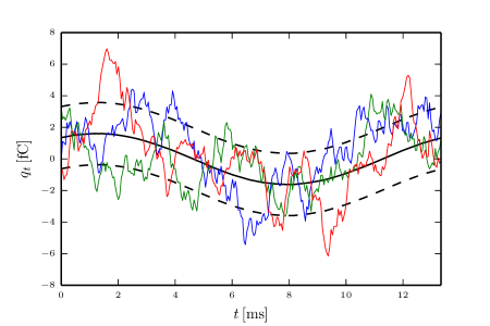
Figure 3: Three example of stochastic trajectories during one period of the driving signal (red, green and blue strongly fluctuating lines). The black solid line represents the ensemble average $\langle q_{t}\rangle$ and the black dashed lines represent the ensemble average plus and minus one standard deviation $\sigma_{t}=\sqrt{\left\langle(q_{t}-\langle q_{t}\rangle)^{2}\right\rangle}$. In this example, the driving frequency is $f_{\rm d}=75\,\textrm{Hz}$ and the amplitude of the driving is $q_{\rm max}^{*}=2.3\,\textrm{fC}$. The average and standard deviation are estimated from 38164 trajectories.

In figure 3, we plot three examples of realizations of the stochastic trajectory $q_{t}$, together with the ensemble average.

3.2 Protocol

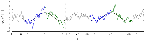
Figure 4: Construction of the ensemble of non-equilibrium trajectories for a process duration of $\tau=8.4\,{\rm ms}$ from a long stationary trajectory driven at $f_{\rm d}=75\,\textrm{Hz}$. Since $\tau<1/f_{\rm d}=13.3\,\textrm{ms}$, we set $\tau_{\rm d}=1/f_{\rm d}$. The smoothly oscillating thick curve represents the control parameter $q_{t}^{*}$. The strongly fluctuating thin curve represents $q_{t}$. The blue portions correspond to members of the forward ensemble and the green portions to members of the backward ensemble. The forward trajectories start at time $(2n+1)\tau_{\rm d}-\tau$ and end at time $(2n+1)\tau_{\rm d}$, and the backward trajectories start at time $(2n+1)\tau_{\rm d}$ and end at time $(2n+1)\tau_{\rm d}-\tau$, where $n$ is an integer (here, we plot $n=0$ and $n=1$). Due to the periodicity of the driving protocol, each member of the forward ensemble is subject to the same driving signal and due to the symmetry of the driving signal, the protocol in each backward process is the time reverse of the protocol in the forward process.

After a transient that we do not analyze here, the system relaxes towards a time periodic stationary state. In other words, the probability distribution $\rho(q,t)$ of the charge $q$ at time $t$ is time periodic of period $1/f_{\rm d}$, the period of the driving signal. We use this periodicity of $\rho(q,t)$ to construct an ensemble of non-equilibrium trajectories.

Here is how we construct the ensembles of forward and backward trajectories of duration $\tau$ from a long quasistationary trajectory $\{q_{t}\}$. We chose the origin of time such that $q_{t}^{*}=q^{*}_{\rm max}\cos(\omega t)$, where $\omega=2\pi f_{\rm d}$. Let $\tau_{\rm d}\geq\tau$ be an integer multiple of the driving period $1/f_{\rm d}$. The $n^{\rm th}$ member of the forward ensemble is the portion of $\{q_{t}\}$ where $(2n+1)\tau_{\rm d}-\tau\leq t\leq(2n+1)\tau_{\rm d}$, $n$ being an integer. The corresponding member of the backward ensemble is the portion of $\{q_{t}\}$ where $(2n+1)\tau_{\rm d}\leq t\leq(2n+1)\tau_{\rm d}+\tau$.

On figure 4, we sketch how the first two members of the forward and backward ensembles are obtained for $\tau_{\rm d}=1/f_{\rm d}$. The blue portions correspond to members of the forward ensemble and the green portions to members of the backward ensemble. The smoothly oscillating curve represents the driving signal $q^{*}_{t}$ and the strongly fluctuating curve is $q_{t}$.

Due to the periodicity of the driving protocol, all the members of the forward ensemble are subjected to the same driving signal. Moreover, since $\rho(q,t)$ is time periodic of period $\tau_{\rm d}$, all the initial mesoscopic states of the forward trajectories are drawn from the same initial distribution $\rho_{0}(q)$ and hence all the forward trajectories are drawn from the same path distribution ${\mathcal{P}}_{\rm F}$. The same reasoning applies the backward trajectories: their initial mesoscopic state is drawn from the same distribution $\rho_{1}(q)$ and they are all submitted to the same driving. Hence they are all drawn from the same path distribution ${\mathcal{P}}_{\rm B}$. Finally, the origin of time was chosen such that $q_{t}^{*}$ is symmetric around $n\tau_{\rm d}$, $q^{*}_{n\tau_{\rm d}-t}=q^{*}_{n\tau_{\rm d}+t}$. Hence the members of the backward ensemble are subjected to a driving that is the time reversal of the driving under which the members of the forward ensemble are submitted.

3.3 Measurement of stochastic entropy production

The amount of entropy produced along a stochastic trajectory ${\bf m}$ is calculated using (3): $\Delta S_{\rm tot}[{\bf m}]=Q[{\bf m}]/T+\Delta S[{\bf m}]$. Following Sekimoto [17], the heat released to the environment in the time interval $[t,t+dt]$ is given by

$${\rm d}Q_{t}=\left(R\frac{{\rm d}q_{t}}{{\rm d}t}+\delta V_{t}\right)\circ{\rm d}q_{t}=-\frac{1}{C}\left(q_{t}-q_{t}^{\star}\right)\circ{\rm d}q_{t},$$ (22)

where $\circ$ denotes Stratonovich product and the second equality is consequence of (21). Note that the amount of heat released per unit time is the sum of two contributions, $\dot{Q}_{t}=\dot{Q}_{t}^{\rm Joule}+\dot{Q}_{t}^{\rm thermal}$. The first contribution is due to the Joule heating inside the resistor: $\dot{Q}_{t}^{\rm Joule}=Ri_{t}^{2}$, and the second to the power injected by thermal fluctuations: $\dot{Q}_{t}^{\rm thermal}=\delta V_{t}i_{t}$. The heat dissipated between times $t_{0}$ and $t_{1}$ along a stochastic trajectory ${\bf m}$ equals to

$$Q[{\bf m}]=\int_{t_{0}}^{t_{1}}{\rm d}Q_{t}=-\int_{t_{0}}^{t_{1}}\frac{q_{t}-q_{t}^{*}}{C}\circ{\rm d}q_{t},$$ (23)

which is measured from the stochastic trajectories.

The trajectory dependent entropy is given by $S(q_{t},t)=-k_{\rm B}\log\rho(q_{t},t)$, where $\rho(q_{t},t)$ is the probability distribution of the charge $q_{t}$ at time $t$. The distribution $\rho(q_{t},t)$ is estimated from the ensemble of trajectories. The system’s entropy change along a trajectory ${\bf m}$ that starts at $q_{0}$ at time $t_{0}$ and ends at $q_{1}$ at time $t_{1}$ is obtained as

$$\Delta S[{\bf m}]=S(q_{1},t_{1})-S(q_{0},t_{0})=-k_{\rm B}\log\rho(q_{1},t_{1})+k_{\rm B}\log\rho(q_{0},t_{0}).$$ (24)

4 Experimental results

Figures 5 and 6 summarize the thermodynamics of the process as a function of the process duration $\tau$ for a driving frequency of $f_{\rm d}=75\,\textrm{Hz}$, and hence a driving period of $1/f_{\rm d}\approx 13.3\,\textrm{ms}$, and a driving amplitude of $q^{*}_{\rm max}=2.3\,\textrm{fC}$. We consider durations up to one period of the driving signal and hence we set $\tau_{\rm d}=1/f_{\rm d}$. The signal $q_{t}$ was sampled at $20\,\textrm{kHz}$ and the ensemble consists of 38164 trajectories.

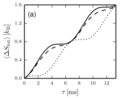
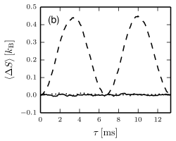
Figure 5: (a) Average entropy production as a function of the process duration $\tau$. The solid line represents the entropy production in the forward process, the dotted line the entropy production in the backward process and the dashed line the conjugated entropy production $\tilde{\Delta S_{\rm tot}}[\bar{\bf m}]$. (b) Average variation of the entropy of the system in the forward (solid line) and in the time reverse process (dotted line). They are both equal to zero for all $\tau$. The dashed line represents the average of $\Delta\tilde{S}[\bar{\bf m}]$ over the time reverse process.

Figure 5a shows the ensemble averages of the amount of entropy produced in the forward process, $\langle\Delta S_{\rm tot}\rangle$ (solid line), the amount of entropy produced in the backward process $\langle\Delta S_{\rm tot}^{\rm B}\rangle$ (dotted line) and of the conjugated entropy production $\langle\tilde{\Delta S_{\rm tot}}\rangle$ (dashed line) as a function of the process duration $\tau$. These three quantities increase with $\tau$, in a manner that is roughly linear with a periodic modulation. We check the inequality (16), $\langle\tilde{\Delta S_{\rm tot}}\rangle\geq\langle\Delta S_{\rm tot}^{\rm B}\rangle$. Moreover, the average amount of entropy produced in the forward process is approximately equal to the average conjugated entropy production, $\langle\Delta S_{\rm tot}\rangle\approx\langle\tilde{\Delta S_{\rm tot}}\rangle$.

We also investigate the average value of the system’s entropy change (figure 5b) in the forward process, $\langle\Delta S\rangle$ (solid line), in the time reverse $\langle\Delta S_{\rm B}\rangle$ (dotted line) and the quantity $\langle\Delta\tilde{S}\rangle$ (dashed line) as a function of the process duration $\tau$. The system’s entropy change vanishes on average both in forward and backward processes. Hence, the average entropy production is equal to the average dissipated heat in both cases, $\langle\Delta S_{\rm tot}\rangle=\langle Q\rangle/T$ and $\langle\Delta S_{\rm tot}^{\rm B}\rangle=\langle Q_{\rm B}\rangle/T$.

In this situation (15) and (16) imply

$$\langle\tilde{\Delta S_{\rm tot}}\rangle-\langle\Delta S_{\rm tot}^{\rm B}\rangle=\langle\Delta\tilde{S}\rangle=k_{\rm B}\int\rho_{2}(q)\log\frac{\rho_{2}(q)}{\rho_{0}(q)}\,{\rm d}q\geq 0.$$ (25)

On figure 5b we can see that $\langle\Delta\tilde{S}\rangle$ is non negative for all $\tau$, in accordance with (25). The quantity $\langle\Delta\tilde{S}\rangle$ is zero for $\tau=0$, $\tau=\tau_{\rm d}/2\approx 6.5\,{\rm ms}$ and $\tau=\tau_{\rm d}$, implying that for these durations, $\rho_{2}\equiv\rho_{0}$. In fact, for $\tau=0$, we have $t_{0}=t_{1}=t_{2}$ and there is no process and hence $\rho_{0}\equiv\rho_{1}\equiv\rho_{2}$. For $\tau=\tau_{\rm d}/2$, we have $t_{2}-t_{0}=\tau_{\rm d}$, and hence $\rho_{2}(q)=\rho(q,t_{0}+\tau_{\rm d})=\rho(q,t_{0})=\rho_{0}(q)$ because $\rho(q,t)$ is time periodic with period $\tau_{\rm d}$. The same reasoning applies for $\tau=\tau_{\rm d}$. In that case, we have $t_{2}-t_{0}=2\tau_{\rm d}$, and hence $\rho_{2}(q)=\rho(q,t_{0}+2\tau_{\rm d})=\rho(q,t_{0})=\rho_{0}(q)$. The quantity $\langle\Delta\tilde{S}\rangle$ is also zero for $\tau=\tau_{\rm d}/2\approx 6.5\,{\rm ms}$ which is one half of the driving period. Finally, $\langle\Delta\tilde{S}\rangle$ is maximum for $\tau\approx 3.3\,{\rm ms}$ and $\tau\approx 10\,{\rm ms}$ which correspond to one fourth and three fourth of the driving period.

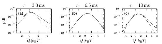
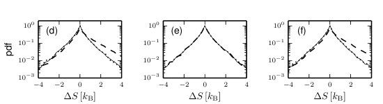
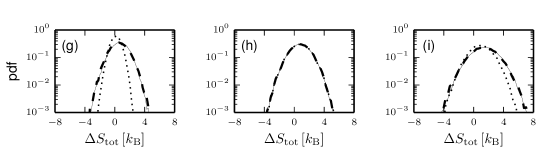
Figure 6: Distributions of the heat (top), system entropy variation (middle) and entropy production (bottom) for the three different durations $\tau\approx 3.3$, $6.5$ and $10\,{\rm ms}$ corresponding respectively to one quarter, one half and three quarters of the driving period $\tau_{\rm d}$. Each column corresponds to one value of $\tau$. Upper row (panels a, b, and c): Distributions of the heat dissipated in the forward (solid lines) and time reverse process (dashed lines). Middle row (panels d, e, and f): Distributions of the variation of the entropy of the system in the forward process (solid lines), in the time reverse process (dotted lines) and of $\Delta\tilde{S}[\bar{\bf m}]$ given by (14) in the time reverse process (dashed lines). Lower row (panels g, h, and i): Distribution $P(\Delta S_{\rm tot})$ of the entropy produced in the forward process (solid lines), distribution ${\rm Phys.~{}Rev.~{}B}(\Delta S_{\rm tot})$ of the entropy produced in the backward process (dotted lines), and distribution $\tilde{P}(\Delta S_{\rm tot})$ of the conjugated entropy production (dashed lines).

On figure 6, we show the distributions of the thermodynamic quantities heat, entropy variation and entropy production in the forward and backward process for the three durations $\tau\approx 3.3$, $6.5$ and $10\,{\rm ms}$, corresponding to one quarter, one half and three quarters of the period of the driving signal.

The first row of figure 6 (panels a, b, and c) shows the distributions of the heat released to the environment in the forward (solid lines) and in the time reverse process (dashed lines). These are identical for $\tau\approx 6.5\,{\rm ms}$ otherwise they are different.

In the middle row (panels d, e and f), we show the distributions of the system’s entropy change in the forward process (solid lines) in the backward process (dotted lines) and of the quantity $\Delta\tilde{S}$ (dashed lines). The distributions of the system’s entropy change in forward and backward processes are identical. They are symmetric with respect to $0$ and non-Gaussian for all values of $\tau$. Similar results were also found in [29, 32] The distribution of $\Delta\tilde{S}[\bar{\bf m}]$ differs from the two others except for $\tau\approx 6.5\,{\rm ms}$.

The lower row (panels g, h and i) of figure 6 shows the distribution $P(\Delta S_{\rm tot})$ of the entropy produced in the forward process (solid lines), the distribution ${\rm Phys.~{}Rev.~{}B}(\Delta S_{\rm tot})$ of the entropy produced in the backward process (dotted lines) and the distribution $\tilde{P}(\Delta S_{\rm tot})$ of the conjugated entropy production (dashed lines). The three distributions are Gaussian, as in [29]. The distributions of the entropy produced in the forward process and of the conjugated entropy production are equal, $P(\Delta S_{\rm tot})=\tilde{P}(\Delta S_{\rm tot})$. The distribution ${\rm Phys.~{}Rev.~{}B}(\Delta S_{\rm tot})$ of the entropy produced in the backward process is equal to the two others for $\tau=6.5\,{\rm ms}$, otherwise it has a different shape. In accordance with equation (16) and with figure 5a, its mean is smaller than the mean of the two others. Moreover, its variance is also smaller. Note that a necessary condition for the fluctuation theorem (1) to hold when the distributions $P(\Delta S_{\rm tot})$ and $\tilde{P}(\Delta S_{\rm tot})$ are Gaussian is that they are equal [26, 41].

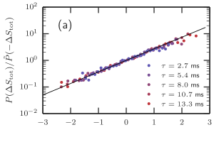
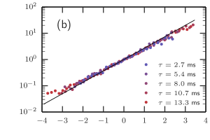
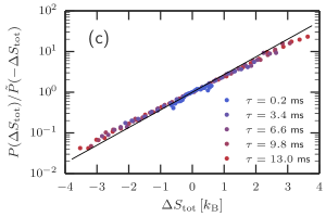
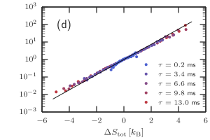
Figure 7: Ratio $P(\Delta S_{\rm tot})/\tilde{P}(-\Delta S_{\rm tot})$ on a logarithmic scale as a function of $\Delta S_{\rm tot}$ for different driving frequencies, amplitudes and durations $\tau$. The black line corresponds to the theoretical prediction $\exp(\Delta S_{\rm tot}/k_{\rm B})$. Panel (a): Driving frequency $f_{\rm d}=75\,\textrm{Hz}$, period $1/f_{\rm d}=13.3\,\textrm{ms}$, amplitude $q^{*}_{\rm max}=1.4\,\textrm{fC}$. Panel (b): Driving frequency $f_{\rm d}=75\,\textrm{Hz}$, period $1/f_{\rm d}=13.3\,\textrm{ms}$, amplitude $q^{*}_{\rm max}=2.3\,\textrm{fC}$. Panel (c): Driving frequency $f_{\rm d}=1\,\textrm{kHz}$, period $1/f_{\rm d}=1\,\textrm{ms}\approx RC$, amplitude $q^{*}_{\rm max}=0.86\,\textrm{fC}$. Panel (d): Driving frequency $f_{\rm d}=1\,\textrm{kHz}$, period $1/f_{\rm d}=1\,\textrm{ms}\approx RC$, amplitude $q^{*}_{\rm max}=1.3\,\textrm{fC}$. For panels (c) and (d), we considered durations up to 13 driving periods, hence $\tau_{\rm d}=13\,\textrm{ms}$.

Figure 7 shows that the theorem (1) is verified with high accuracy in our experiment. This figure shows the ratio $P(\Delta S_{\rm tot})/\tilde{P}(-\Delta S_{\rm tot})$ between the distribution $P(\Delta S_{\rm tot})$ of the entropy produced in the forward process and of the distribution $\tilde{P}(-\Delta S_{\rm tot})$ of (minus) the conjugated entropy production $-\tilde{\Delta S_{\rm tot}}[\bar{\bf m}]$ for the backward process for different driving frequencies and amplitudes and for the durations. Panels (a) and (b) correspond to a driving frequency of $f_{\rm d}=75\,\textrm{Hz}$ and hence a driving period of $1/f_{\rm d}=13.3\,\textrm{ms}$. The signal $q_{t}$ was sampled at $20\,\textrm{kHz}$. The driving amplitudes are $q^{*}_{\rm max}=1.4\,\textrm{fC}$ for panel (a) and $q^{*}_{\rm max}=2.3\,\textrm{fC}$ for panel (b). The ensembles consist of $38\,424$ (panel a) and $38\,164$ (panel b) trajectories. Panels (c) and (d) correspond to a driving frequency of $f_{\rm d}=1\,\textrm{kHz}$ and hence the driving period is $1/f_{\rm d}=1\,\textrm{ms}\approx RC$, which is the time constant of the circuit. Here, we considered process durations up to 13 periods, and hence $\tau_{\rm d}=13/f_{\rm d}=13\,\textrm{ms}$. The signal $q_{t}$ was sampled at $100\,\textrm{kHz}$ and the ensembles consist of $198\,144$ trajectories. The driving amplitudes are $q_{\rm max}^{*}=0.86\,\textrm{fC}$ for panel (c) and $q_{\rm max}^{*}=1.3\,\textrm{fC}$ for panel (d). The black solid line corresponds to the theory, $\exp\left(\Delta S_{\rm tot}/k_{\rm B}\right)$. The fluctuation theorem (1) is fulfilled with high accuracy (along up to four decades) for all the durations considered.

5 Conclusion

To summarize, in this work we have studied experimentally the thermodynamics of the transition between two non-equilibrium states in a parallel $RC$ circuit, in the light of the fluctuation theorem for the entropy production (1). In such a situation, the fluctuation theorem (1) presents a subtlety: for the backward process it involves the distribution of the conjugated entropy production (6) rather than the distribution of the entropy production.

We have characterized the statistics of the heat dissipation, entropy variation and entropy production in the forward and backward processes. In particular, for the backward process, we have studied the difference between entropy production and conjugated entropy production. Furthermore, we have verified that the detailed fluctuation theorem is fulfilled with high accuracy for different driving frequencies and amplitude and for different process durations, which confirms the universality of the result.

References

- [1] Szilard L 1925 Z. Physik 32 753–788 ISSN 0044-3328
- [2] Wang G M, Sevick E M, Mittag E, Searles D J and Evans D J 2002 Phys. Rev. Lett. 89 050601
- [3] Collin D, Ritort F, Jarzynski C, Smith S B, Tinoco I and Bustamante C 2005 Nature 437 231–234 ISSN 0028-0836
- [4] Evans D J, Cohen E G D and Morriss G P 1993 Phys. Rev. Lett. 71 2401–2404
- [5] Gallavotti G and Cohen E G D 1995 Phys. Rev. Lett. 74 2694–2697
- [6] Jarzynski C 1997 Phys. Rev. Lett. 78 2690–2693
- [7] Crooks G E 1998 Journal of Statistical Physics 90 1481–1487 ISSN 0022-4715, 1572-9613
- [8] Crooks G E 1999 Phys. Rev. E 60 2721–2726
- [9] Hatano T and Sasa S i 2001 Phys. Rev. Lett. 86 3463–3466
- [10] Seifert U 2005 Phys. Rev. Lett. 95 040602
- [11] Harris R J and Schütz G M 2007 J. Stat. Mech. 2007 P07020 ISSN 1742-5468
- [12] Saha A, Lahiri S and Jayannavar A M 2009 Phys. Rev. E 80 011117
- [13] Esposito M and Van den Broeck C 2010 Phys. Rev. Lett. 104 090601
- [14] Spinney R E and Ford I J 2012 Fluctuation relations: a pedagogical overview Nonequilibrium Statistical Physics of Small Systems: Fluctuation Relations and Beyond (Weinheim: Wiley-VCH) ISBN 978-3-527-41094-1 arXiv: 1201.6381 URL http://arxiv.org/abs/1201.6381
- [15] Sekimoto K 1998 Prog. Theor. Phys. Supplement 130 17–27 ISSN 0375-9687,
- [16] Esposito M and Broeck C V d 2011 EPL 95 40004 ISSN 0295-5075
- [17] Sekimoto K 2012 Stochastic Energetics edición: 2010 ed (Springer) ISBN 9783642262685
- [18] Seifert U 2012 Reports on Progress in Physics 75 126001 ISSN 0034-4885, 1361-6633
- [19] Deffner S and Lutz E 2012 arXiv:1201.3888 [cond-mat] ArXiv: 1201.3888
- [20] Granger L 2013 Irreversibility and information Ph.D. thesis Technische Universität Dresden Dresden, Germany URL http://www.qucosa.de/recherche/frontdoor/?tx_slubopus4frontend%5Bid%5D=14438
- [21] Roldan E 2014 Irreversibility and Dissipation in Microscopic Systems (Springer) ISBN 9783319070797
- [22] Thingna J, Hänggi P, Fazio R and Campisi M 2014 Phys. Rev. B 90 094517
- [23] Bonança M V S and Deffner S 2014 The Journal of Chemical Physics 140 244119 ISSN 0021-9606, 1089-7690
- [24] Liphardt J, Dumont S, Smith S B, Tinoco I and Bustamante C 2002 Science 296 1832–1835 ISSN 0036-8075, 1095-9203
- [25] Trepagnier E H, Jarzynski C, Ritort F, Crooks G E, Bustamante C J and Liphardt J 2004 PNAS 101 15038–15041 ISSN 0027-8424, 1091-6490
- [26] Douarche F, Ciliberto S and Petrosyan A 2005 J. Stat. Mech. 2005 P09011 ISSN 1742-5468
- [27] Tietz C, Schuler S, Speck T, Seifert U and Wrachtrup J 2006 Phys. Rev. Lett. 97 050602
- [28] Andrieux D, Gaspard P, Ciliberto S, Garnier N, Joubaud S and Petrosyan A 2007 Phys. Rev. Lett. 98 150601
- [29] Joubaud S, Garnier N B and Ciliberto S 2008 EPL 82 30007 ISSN 0295-5075
- [30] Mestres P, Martinez I A, Ortiz-Ambriz A, Rica R A and Roldan E 2014 Phys. Rev. E 90 032116
- [31] Koski J V, Sagawa T, Saira O P, Yoon Y, Kutvonen A, Solinas P, Möttönen M, Ala-Nissila T and Pekola J P 2013 Nat Phys 9 644–648 ISSN 1745-2473
- [32] Martínez I A, Roldán É, Dinis L, Petrov D and Rica R A 2015 Phys. Rev. Lett. 114 120601
- [33] Ritort F, Bustamante C and Tinoco I 2002 PNAS 99 13544–13548 ISSN 0027-8424, 1091-6490
- [34] Kawai R, Parrondo J M R and den Broeck C V 2007 Phys. Rev. Lett. 98 080602
- [35] Gomez-Marin A, Parrondo J M R and Broeck C V d 2008 EPL 82 50002 ISSN 0295-5075
- [36] Parrondo J M R, Broeck C V d and Kawai R 2009 New J. Phys. 11 073008 ISSN 1367-2630
- [37] Kurchan J 1998 J. Phys. A: Math. Gen. 31 3719 ISSN 0305-4470
- [38] Cover T M and Thomas J A 1991 Elements of Information Theory 99th ed (New York: Wiley-Interscience) ISBN 9780471062592
- [39] van Zon R, Ciliberto S and Cohen E G D 2004 Phys. Rev. Lett. 92 130601
- [40] Garnier N and Ciliberto S 2005 Phys. Rev. E 71 060101
- [41] Granger L, Niemann M and Kantz H 2010 J. Stat. Mech. 2010 P06029 ISSN 1742-5468