The SFXC software correlator for Very Long Baseline Interferometry: Algorithms and Implementation

Abstract

In this paper a description is given of the SFXC software correlator, developed and maintained at the Joint Institute for VLBI in Europe (JIVE). The software is designed to run on generic Linux-based computing clusters. The correlation algorithm is explained in detail, as are some of the novel modes that software correlation has enabled, such as wide-field VLBI imaging through the use of multiple phase centres and pulsar gating and binning. This is followed by an overview of the software architecture. Finally, the performance of the correlator as a function of number of CPU cores, telescopes and spectral channels is shown.

1 Introduction

Very Long Baseline Interferometry (VLBI) is a technique in which the signals from a network of radio telescopes, spread around the world, are combined to create one single telescope with a resolution far surpassing that of the individual telescopes. This is accomplished by computing the correlation functions on every baseline, formed by all possible pairs of telescopes, on a central data processor called the correlator. The digitised signals are recorded on magnetic media which are shipped to the correlator, or, with the advent of real-time electronic VLBI (e-VLBI) (Szomoru et al, 2006), streamed directly over the Internet. From its inception in 1980 (Porcas, 2010), the European VLBI Network (EVN) has relied on correlators built from dedicated ASIC-based hardware, because the processing of VLBI observations far exceeded the capacity of standard computing components (see e.g. Schilizzi et al (2001)). However, the continuously increasing computing power of modern CPUs has made it possible to use commercial-of-the-shelf (COTS) components for correlation. Together with the increase in storage capacity this has changed the way VLBI is done.

Development of the Super FX Correlator (SFXC) at JIVE started with the purpose to detect and track a spacecraft in the outer solar system, namely ESA’s Huygens Probe as it descended to the surface of Saturn’s moon Titan (Pogrebenko et al, 2004). Such an application of VLBI calls for extremely high spectral resolution and a detailed control of the delay model, both of which were in practice not available in existing hardware correlators. From then on, the SFXC software correlator has been further developed into a very efficient and flexible system, providing a number of completely new observing modes for the EVN.

The introduction of software correlators has brought about several scientific improvements. Although 2-bit representation of the data is still used for economy of storage and transport, the algorithm used for correlation is no longer limited to few-bit precision. This means that the data can be processed with much higher accuracy. In contrast to hardware correlators, software correlators can operate asynchronously, certainly when the data are read from disk systems. The consequence of the above changes is that correlation functions can be obtained with almost arbitrary windowing functions and accumulation times. This results in a much extended coverage of parameter space, providing for example arbitrarily fine spectral resolution and very flexible pulsar gating and binning.

In addition, the software correlator has far more flexible interfaces to data sources, geometric model components and data output, as these are now entirely implemented in software. The software correlator is therefore a natural platform to process real-time e-VLBI data. The flexible interfaces also make it possible to cross-correlate different data formats, compensate for problems with recording times and implement multiple output streams for more than one target position within the field of view of the observations (e.g. Cao et al, 2014).

The software correlator runs on a standard Linux cluster and has become the operational correlator for all EVN operations at JIVE. SFXC is available under version 2 of the GNU Public License (GPL). It has proven to be a very stable platform, routinely producing high- quality scientific results for the EVN community. In almost all aspects it compares favourably to the old MkIV EVN hardware correlator (Schilizzi et al, 2001). It should finally be noted that power consumption is higher for software correlators, this situation will improve with time as the drive towards green computing produces ever more efficient processors.

A number of other VLBI software correlators have been developed over the past decade. Some examples are the K5 software correlator, of the Japanese National Institute of Information and Communications Technology (NICT) (Kondo et al, 2004), used mainly for geodetic applications, the SOFTC correlator (Lowe, 2004), which is the operational VLBI correlator of the Jet Propulsion Laboratory (JPL), and the DiFX correlator (Deller et al, 2007, 2011), maintained by an international consortium of developers and used at a number of sites such as the Very Long Baseline Array (VLBA), Australian Long Baseline Array (LBA), and the Max Planck Institute for Radio Astronomy (MPIfR).

2 Correlation algorithm

Figure 1: The data flow inside a correlator node.

In this section we present the correlation algorithm implemented in SFXC. We will limit the discussion to our design considerations. A more in-depth review of radio interferometry and VLBI can be found in standard references like e.g.  Thompson et al (2001) and Taylor et al (1999). In Fig. 1 the data flow inside the correlator core is shown and in the following subsections we shall elaborate on each step in this flow.

2.1 Delay compensation

Prior to cross correlation the signals from each antenna must be brought to a common frame of reference. For most applications this is the geocentric frame. This is accomplished by time-shifting the signals from each antenna such that at all signals track the same wave front. The default delay model used in SFXC is the CALC 10 software developed at the Goddard Space Flight Center. This is the same model that was used for the EVN MkIV correlator at JIVE (Schilizzi et al, 2001). The default delay model can overridden by a user supplied model. For instance, Duev et al (2012, 2015) developed a near-field delay model for spacecraft tracking applications in combination with SFXC and a delay model that has been successfully used to correlate data observed with the RadioAstron orbital telescope. Before correlation the delay model is evaluated at one second intervals, which allows the model to be interpolated close to the machine precision (Özdemir, 2007). During correlation these values are interpolated using an Akima spline (Akima, 1970). The Akima spline was chosen because it yields accurate results also at the edges of the interpolation interval.

Compensation for the geometric delay $\tau$ is performed in two steps. In the first step the input stream is shifted by an integer number of samples. For a Nyquist sampled signal the corresponding delay $\tau_{i}$, called the integer delay, rounding to the nearest integer,

$$\tau_{i}=\mathtt{round}(2B\tau)/2B,$$ (1)

with $B$ the sampled bandwidth. The residual fractional delay, given by

$$\tau_{f}=\tau-\tau_{i},$$ (2)

is at most half a sample period. The fractional delay leads to a phase error across the band

$$\phi_{\mathrm{frac}}(\nu)=2\pi\tau_{f}\nu,$$ (3)

where $\nu$ is the baseband frequency. In order to remove the fractional delay error, the data is divided into segments of $N$ samples, each segment is Fourier transformed, and the resulting spectra are multiplied by $e^{-i\phi_{\mathrm{frac}}}$. We will discuss the choice of the segment length $N$ later in this section.

The astronomical signal as it is received by a telescope is down converted from a frequency range $\nu_{sky}\leq\nu<\nu_{sky}+B$ to a range $0\leq\nu<B$, the so-called baseband. Since the fractional delay compensation is performed on the base band signal a phase error $\phi_{\mathrm{frot}}$ will remain:

$$\phi_{\mathrm{frot}}=2\pi\nu_{\mathrm{sky}}\tau.$$ (4)

The effect of $\phi_{\mathrm{frot}}$ is most easily shown by looking at a single baseline. Let $\tau_{b}$ be the delay between the two telescopes on that baseline. If $\phi_{\mathrm{frot}}$ is not corrected, the fringe amplitudes on this baseline will oscillate with a frequency $\nu_{\mathrm{sky}}\textrm{d}\tau_{b}/\textrm{d}t$. This effect is removed by multiplying the time domain baseband voltage data for each antenna with $e^{-i\phi_{\mathrm{frot}}}$, a process which is called fringe rotation or fringe stopping.

If the delay $\tau$ were constant then the combination of delay compensation and fringe rotation would exactly compensate for the difference in arrival time $\tau$. In the general time dependent case this correction is only exact for a single frequency $\nu_{\mathrm{frot}}$, which we call the fringe rotation frequency. In Eq. (3) and Eq. (4) the fringe rotation frequency is at the band edge, $\nu_{\mathrm{frot}}=\nu_{\mathrm{sky}}$. The fringe rotation frequency can be shifted by an arbitrary amount $\nu_{\delta}$ by applying a phase shift

$$\psi(\nu_{\delta})=e^{-i2\pi\nu_{\delta}\tau}.$$ (5)

which will shift the fringe rotation frequency to $\nu_{\mathrm{frot}}=\nu_{\mathrm{sky}}+\nu_{\delta}$. The phase shift that should be applied in the fringe rotator then becomes

$$\phi_{\mathrm{frot}}(\nu_{\delta})=2\pi(\nu_{\mathrm{sky}}+\nu_{\delta})\tau=2\pi\nu_{\mathrm{frot}}\tau.$$ (6)

In principle $\nu_{\delta}$ could be chosen to align with a spectral line to maximize the signal to noise at this spectral point. In SFXC we set $\nu_{\delta}$ equal to $B/2$ which moves $\nu_{\mathrm{frot}}$ to the centre of the band, minimizing the average error.

The act of delay compensation and fringe rotation is equivalent to applying a Lorentz transformation, transforming the signal from the reference frame of each telescope to that of a fictional observer at the geocentre. At this point the data can be re-analysed at an arbitrary spectral resolution, unrelated to that used in the delay compensation. This decoupling of spectral resolution in the delay compensation and cross-correlations is essential to achieve true arbitrary spectral resolution.

In the fractional delay correction a single delay value is used for an entire FFT segment, which constrains the FFT period to some fraction of the time between two integer delay changes. On short time scales the delay $\tau(t)$ is approximately linear

$$\tau(t)\approx\tau_{0}+(t-t_{0})\dot{\tau},$$ (7)

where $\tau_{0}$ is the delay at the time $t_{0}$, and $\dot{\tau}$ is the delay rate. The number of samples $N$ between two integer delay changes is independent of bandwidth and is given by

$$N=\dot{\tau}^{-1}.$$ (8)

Following the discussing in Sec. 9.7 of Thompson et al (2001), the drift in delay during the FFT period will cause a loss in amplitude of,

$$L(\nu)=\frac{\sin({\pi(\nu-B/2)\dot{\tau}T})}{\pi(\nu-B/2)\dot{\tau}T},$$ (9)

where $\nu$ is the baseband frequency, $B$ the bandwidth, and $T$ the duration of the FFT. Additionally, there will be a negligible phase error proportional to $\ddot{\tau}T^{2}$. On terrestrial baselines the maximum geometric delay rate that can be encountered is $\dot{\tau}_{t}=1.5\mu s/s$. In order to keep the drift in delay over one FFT segment within 0.1 samples, the maximum FFT size, rounding down to a power of two, is  $N_{max}=65536$ samples. For near-field VLBI the delay rates can be considerably higher. For example satellites in a low earth orbit move at velocities of up to 8 km/s, which translates to a delay rate of $\dot{\tau}=27\mu s/s$. For such satellites the maximum FFT window size becomes $N_{max}=2048$.

2.2 Windowing

An FX correlator, such as SFXC, computes a cyclical correlation function rather than a linear correlation. This is a direct consequence of the discrete correlation theorem

$$\Gamma[m]=\sum_{n=0}^{N-1}f[(n+m)\textrm{mod}N]g^{*}[n]=\sum_{k=0}^{N-1}F[k]G^{*}[k]e^{i2\pi km/N},$$ (10)

where $N$ is the FFT size and $F[k](G[k])$ is the Fourier pair of $f[n](g[n])$. By applying an appropriate windowing function this cyclicity can be reduced or even removed completely.

At the windowing stage, the data stream of each telescope is divided into segments of $N$ samples which are then multiplied by a windowing function. These windowed segments are then Fourier transformed and the cross-correlations product are computed. Consecutive segments are half-overlapped.

The cross-correlation function after applying a windowing function $w[n]$ becomes

$$\Gamma[m]=(w[n]\cdot f[n])\ast(w[n]\cdot g^{*}[n])=\mathcal{F}^{-1}\left(W^{2}[k]\ast(F[k]\cdot G^{*}[k])\right),$$ (11)

where $W[k]$ is the Fourier pair of $w[n]$. This means that the spectrum is convolved with the square of the Fourier transform of the windowing function.

The choice of window function is a compromise between spectral leakage effects and spectral resolution. E.g. the square window defined by

$$w[n]=\left\{\begin{array}[]{l l l}1&&n<=N/2\\ 0&&n>N/2\end{array}\right.$$ (12)

convolves the spectrum of the cross-correlation function with a $\textrm{sinc}^{2}$ function. The sinc function has a narrow main lobe and therefore excellent resolution, but large slowly decaying side lobes which can potentially obscure spectral line features. This ringing effect is due to the hard edge at $n=N/2$. Smoother windows, such as the Hann window, will reduce leakage effects but at the cost of resolution. The loss in resolution can be compensated by increasing the number of spectral points, but this in turn leads to larger output data volumes. The windowing functions that are currently available in SFXC and their most important characteristics are listed in Table 1.

Window name	Definition	Main lobe FWHM	First side lobe
Square	$w[n]=1$ if $n<=N/2$ else $0$	1.21	-13 dB
Cosine	$w[n]=\cos(\pi n/(N-1))$	1.64	-23 dB
Hann	$w[n]=0.5(1-\cos(2\pi n/(N-1))$	2.00	-31 dB
Hamming	$w[n]=0.54-0.46\,\cos(2\pi n/(N-1))$	1.82	-43 dB

Table 1: Available window functions and their characteristics

2.3 Cross-correlation and normalization

In the final step auto- and cross-correlations are computed for all baselines. Whether to compute cross-hand polarisations or only parallel polarisations is a user configurable option. The requested correlation products are accumulated in a buffer until the end of the integration period after which they are written to disk. The correlator integration time is defined according to the scientific goals of the observations. For regular VLBI projects it is typically 1-4s, but can be much shorter e.g. for wide field of view applications.

At the end of the integration period, the visibilities are normalized.

According to the Wiener-Khinchin theorem the total power contained in a signal can be obtained from the auto-correlations. If $P_{i}$ is the total power of telescope $i$, the normalisation factor for baseline pair $(i,j)$ will be

$$A_{ij}=\sqrt{P_{i}P_{j}}.$$ (13)

In practice the computation of the normalisation factor is complicated by the fact that a certain fraction of the input samples may be absent. This for example can be caused by a faulty hard drive or missing network packets. Furthermore, some data formats use data replacing headers and therefore will have missing samples even in the absence of any disk or network failures. Missing samples are flagged and replaced with zeros and will therefore not contribute to the cross-correlations. If during some period of time one telescope has invalid data but the other does not then Eq. (13) will overestimate the cross-spectrum power. The normalization factor should be scaled by an additional factor

$$C_{ij}=N^{(ij)}_{\textrm{bl}}/N^{(i)}_{\textrm{valid}},$$ (14)

where $N^{(ij)}_{\textrm{bl}}$ is the number of samples for which both telescopes on the baseline simultaneously have valid data, and $N^{(i)}_{\textrm{valid}}$ is the total number of valid samples for telescope $i$. The normalisation factor then becomes

$$A_{ij}=\sqrt{C_{ij}C_{ji}P_{i}P_{j}}.$$ (15)

3 Pulsar binning

In this section we will discuss the various aspects relating to the correlation of pulsar data. A fundamental property of pulsars is that although their individual pulses can have widely varying pulse shapes and arrival times, the long term average pulse profile is highly stable (Lorimer and Kramer, 2005). Due to this property high precision models of the pulsar rotational phase can be created. For many pulsars the duty cycle, $\tau_{d}$, defined as the ratio between pulse width and pulse period, is relatively small. A significant improvement in signal to noise for VLBI observations can be achieved by accumulating the correlation function only during pulse reception. This is commonly referred to as pulsar gating. Using this approach the signal to noise can be increased by approximately $\sqrt{1/\tau_{d}}$, which typically is a factor of 3-5.

A closely related concept is pulsar binning. Here the pulse period is divided into a number of time bins and the correlation function is accumulated individually for each bin. In SFXC the user specifies a gating interval together with the number of bins to be placed equidistantly within this interval. In this implementation pulsar gating is merely a special case of pulsar binning. In Fig. 2 we show an example pulse profile of pulsar B0329+54 which was produced using the pulsar binning mode.

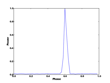
(a) (a)

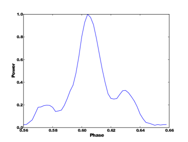
(b) (b)

Figure 2: (a) Pulse profile for B0329+54 obtained from 50 bins across the full period. The profile is obtained from the total power in each bin on the Effelsberg-Westerbork baseline. (b) same as (a) but with 50 bins across the pulse.

Pulsar binning requires that a model of the target pulsar is available, and therefore that it has already been studied in a pulsar timing experiment. For SFXC the pulsar model is supplied in the form of a tempo(2) polyco file (Hobbs et al, 2006). The polyco file contains a polynomial model of the pulsar phase as a function of time for a certain site and for a single frequency. SFXC requires the polyco file to be generated for the geocentre.

An important consideration in pulsar observations is the dispersion caused by the interstellar medium. The difference in arrival times (in ms) between two frequencies $\nu_{1}$ and $\nu_{2}$ (in MHz) is (Lorimer and Kramer, 2005)

$$\Delta{t}\approx 4.15\times 10^{6}\times DM\times(\nu_{1}^{-2}-\nu_{2}^{-2})\quad[\textrm{ms}],$$ (16)

where $DM$ is the dispersion measure. The dispersion measure is defined as the integrated electron density along the line of sight to the pulsar. For some millisecond pulsars this dispersive effect can be significant even within a single frequency band. For example the difference between the arrival times of the highest and lowest frequency across an 8 MHz band at 21 cm for pulsar B1937+21 is 1.7 ms, which is larger than the pulse period.

A computationally inexpensive method to de-disperse a signal is incoherent de-dispersion. Because the dispersive delay is equal for all telescopes, incoherent de-dispersion can be applied post correlation. The cross-correlations are performed at high enough spectral resolution such that within a single frequency channel the dispersive delay is not significant. Each spectral point is then added to the correct pulsar bin by time shifting it according to Eq. (16). This scheme works as long as the length of the FFTs required to reach the needed spectral resolution is smaller than the pulse width.

The dispersive delay can be removed completely using coherent de-dispersion algorithms (Hankins and Rickett, 1975). This involves applying a filter with transfer function

$$H(\nu_{0}+\nu)=\exp{\left(\frac{-i2\pi\nu^{2}DM}{2.41\times 10^{-10}\nu_{0}^{2}(\nu_{0}+\nu)}\right)}$$ (17)

where $\nu_{0}$ is the central frequency of the observing band in MHz, and $|\nu|\leq B/2$ where $B$ is the bandwidth.

Applying a coherent de-dispersion filter comes at considerable computational cost compared to incoherent methods. For the majority of pulsars the incoherent de-dispersion scheme is sufficient. However, for some high-DM millisecond pulsars, coherent de-dispersion is necessary as the size of the FFTs that would be needed to perform incoherent de-dispersion is close to the pulse period. At the time of writing (early 2014), coherent de-dispersion in SFXC was still in the validation phase

4 Wide-field VLBI

Fundamentally, the field of view in a VLBI observation is limited only by the primary antenna beams of the participating telescopes. Provided that sufficient spectral and temporal resolution is available to keep smearing effects at an acceptable level, it is possible to image the entire primary antenna beam. However, this has been done only for a small number of experiments in the past, because of the very large data volumes (see e.g. Lenc et al, 2008; Chi et al, 2013).

A simple "first order" model of a radio dish is that of a uniformly illuminated circular aperture of diameter $d$. The primary beam power $I(\theta)$, as a function of the angle $\theta$ (in radians), is determined by the Fraunhofer diffraction pattern of the aperture and is given by (Born and Wolf, 1999)

$$I(\theta)=\left(\frac{2J_{1}(\pi d\sin(\theta)/\lambda)}{\pi d\sin(\theta)/\lambda}\right)^{2},$$ (18)

where $\lambda$ is the wavelength and $J_{1}(x)$ a Bessel function of the first kind. From Eq. (18) it follows that a circular aperture has its half maximum at $\theta=0.51\lambda/d$ and the first null at $\theta=1.22\lambda/d$. In practice the circular aperture is only an approximation of a real physical dish. The beam shape ultimately has to be determined experimentally and in general is a function of frequency and elevation.

For an interferometer consisting of identical antennas, such as the VLBA, the beam size of the interferometer is equal to the beam size of the individual antennas. For a heterogeneous array such as the EVN the situation is more complicated (Strom, 2004). For example, consider the limiting case where one antenna is much larger than the other dishes in the array and the beams of the smaller antennas can be considered constant over the beam of the larger dish. In this case the size of the interferometer beam is up to 40% larger than the beam of the largest dish in the array (Strom, 2004).

Besides primary beam losses, discretization effects in the correlator also are a source of signal degradation. Two closely related effects are time- and frequency smearing. Both effects are ultimately caused by the fact that the delay model is evaluated for a single point on the sky, the delay tracking centre, but is then applied to the entire field. Time smearing occurs due to the fact that during each integration the correlation function is accumulated over some finite time $T$. Because of the high delay rates in VLBI, contributions from sources which are not close to the delay tracking centre will degrade quickly with $T$. Similarly, frequency smearing is caused by the fact that each spectral channel can be regarded as an average over some bandwidth $\Delta\nu$. If the visibility phase varies significantly over this bandwidth then decorrelation will occur. An in-depth review of time- and frequency smearing can be found in chapter 6 of Thompson et al (2001), and chapters 17 (W.D. Cotton) and 18 (A.H. Bridle and F.R. Schwab) in  Taylor et al (1999).

Because of the need for short integration times and high spectral resolution, conventional wide-field data sets can be very large. For example, to map the primary beam of a 100m telescope at 21cm (9.5 arcmin) with a maximum baseline of 10000 km would require 100ms integrations and 7.8 KHz channel widths to keep smearing losses within 10%. A standard 10 telescope 1 Gb/s EVN observation in this case would produce approximately 3 TB worth of user data in 6 hours. However, in an average field there will only be a few dozen mJy-class sources within the beam of a 100m dish. A more practical approach is to produce a separate narrow field data set for each source in the field rather than a single monolithic wide field data set. This procedure greatly simplifies the data reduction and is known as multiple simultaneous phase centre observing (Deller et al, 2011).

Internally the correlator processes the data at the required high spectral and temporal resolution, performing short sub-integrations. At the end of each sub-integration, the phase centre is shifted to all points of interest. The visibilities for each point of interest are accumulated individually. The results are averaged down in time and frequency before they are written to disk.

The phase centre is shifted from the original phase centre to the target position by applying a phase shift $\phi$ proportional to the difference in geometric delay $\Delta\tau$ between both positions, where (Morgan et al, 2011)

$$\Delta\tau=(\tau^{\prime}-\tau)(1-\dot{\tau}),$$ (19)

here $\tau$ is the delay at the original phase centre, $\tau^{\prime}$ the delay at the target position, and $\dot{\tau}$ the time derivative of $\tau$. The term $(1-\dot{\tau})$ accounts for the change in delay during the period $\tau-\tau^{\prime}$. The phase shift $\phi$ then becomes

$$\phi=2\pi\nu_{\mathrm{sky}}\Delta\tau,$$ (20)

where $\nu_{\mathrm{sky}}$ is the sky frequency.

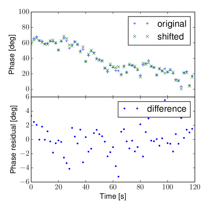
(a) (a)

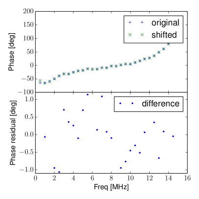
(b) (b)

Figure 3: Comparison between visibility phases obtained using the multiple simultaneous phase centre method and visibilities obtained using a conventional correlation on the Effelsberg - Shanghai baseline (a) Top: phase as a function of time for both datasets. Bottom: Phase difference between both datasets. The visibilities were averaged in frequency over the inner 80% of the band. (b) Phase as a function of frequency, vector averaged over 120 sec.

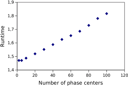
Figure 4: Performance of multiple phase centre correlation normalized to a single phase centre.

We demonstrate the validity of the multiple phase centre method by comparing the following two data sets obtained using target source 3C66A. The first data set was created using a conventional correlation with the delay tracking centre on the target. The second data set was obtained by placing the primary delay tracking centre 3 arcmin away from the target source and obtaining a data set for 3C66A using the multiple phase centre method. In both cases the same raw data were used and the pointing centre of the array coincided with 3C66A. The raw data consists of six 15 minute scans that were distributed evenly over a 6 hour period. For the multiple phase centre correlation, 8192 spectral points and sub-integrations of 25ms were used, keeping smearing effects within 1%. The end result was averaged down to 32 spectral points and 2s integrations. In Fig. 3 we show visibility phase for both datasets for a segment of data on the Effelsberg - Shanghai baseline. Both data sets track the same average phase and the phase difference between both data sets is purely stochastic. Over the whole 6 hour data set we found the average phase difference to be $<\phi_{1}-\phi_{2}>=-0.01$ deg and the standard deviation of the phase difference to be $\sigma_{\phi}=1.7$ deg. This is consistent with the shifted data set having a slightly lower signal to noise but does not imply a significant amount of decorrelation.

Because the phase centre shifting is only performed at the end of each sub-integration period, which is relatively infrequently, the performance scales very well with the number of phase centres. In Fig. 4 we plot the correlation time as function of the number of phase centres. The benchmark was performed using 10 minutes of data at 18 cm using 10 telescopes and a maximum baseline size of 10000 km. Internally 4096 spectral points and 50ms sub-integrations were used, giving a total smearing loss of about 2%. Enabling multiple phase centre correlation increases correlation time by nearly 50%, which is mostly due to the large FFT size needed for this mode. After paying this constant performance penalty, each additional phase centre comes at very little cost. Increasing the number of phase centres from 2 to 100 only increases correlation time by 25%.

5 Software Architecture

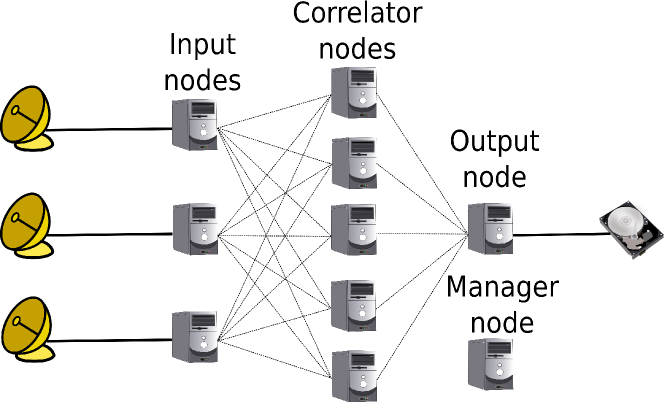
Figure 5: Overview of the SFXC software architecture.

SFXC is a distributed MPI (Message Passing Interface Forum, 2014) application intended to be deployed on a generic Linux computing cluster. The correlator is driven by two configuration files, a VLBI EXperiment (VEX) file and a Correlator Control File (CCF). The VEX file describes the observation as it has been recorded, including the frequency set-up, the scan structure, clock offsets, etc. The VEX files are used by both the telescopes and the correlator. In addition a CCF is supplied to the correlator which includes all parameters specific to a correlation job. These parameters include information such as integration times, data locations, and number of spectral channels. The CCF file is in JSON format which has the benefit of being human readable as well as being easy to parse in software.

In Fig. 5 we show the architecture of SFXC. The MPI processes are divided over a number of specialized nodes, each performing a specific task. There are four types of nodes: input nodes; correlator nodes; one output node; and one manager node.

5.1 Manager node

The manager node controls the correlation process. The input data stream is divided into time slices with a duration equal to the integration time. The main task of the manager node is to assign time slices to correlator nodes. To increase the amount of parallelization each time slice contains data only for a single sub-band. Thus each sub-band is sent to a different correlator node.

Communication between the manager node and the other nodes is done via MPI messages. Whenever a correlator node has nearly finished correlating it will signal the manager node. The manager node will then assign a new time slice to that correlator node so that the correlator node can immediately process a new time slice when it finishes the current time slice. The relevant parameters pertaining to this time slice are passed to the input nodes and the correlator node itself.

When all time slices are processed the manager node will instruct all other nodes to shut down and close the application.

5.2 Input nodes

Figure 6: Example of a multiplexed 8 bits long data word as encountered in disk based data formats. In this example there are two sub-bands, called SB 0 and SB 1. Each sample consists of two bits, a Sign bit and a Magnitude bit. It is the task of the corner turner to split such a word into separate data streams for each sub-band.

An input node reads data from a single data source, corner turns the data into individual sub-bands, and sends the resulting data streams to the correlator nodes. In this process it applies the integer delay correction, as described in Sec. 2. For performance reasons, the data transfers are not done through MPI but via standard TCP connections. The data source can be either a file, a network socket, or a Mark5 diskpack (Whitney, 2003). Currently the Mark4, Mark5B, VLBA, and VDIF dataformats are supported.

Most data formats are multiplexed. This is an artefact from the time when data were recorded onto magnetic tapes. The tape was divided into tracks and each sub-band was split over one or more tracks. In principle the way these sub-bands are divided over the tracks is arbitrary and the exact mapping is recorded in the VEX file. The concept of a track is converted to a disk based format by packing all tracks into a stream of input words. The size of each data word in bits is equal to the number of tracks, with a logical one-to-one mapping of bit location inside a data word to a track number. In this scheme the first track is mapped to bit 0, and so on, as illustrated in Fig.6. Currently only the VDIF format (Whitney et al, 2009) offers the possibility to record each sub-band in a separate data frame and therefore avoid the need for corner turning, although VDIF supports multiplexing as well.

Because the corner turning involves many bitwise operations it is a very costly in terms of processing power. Due to the high data rates in VLBI, typically 1 Gb/s, the corner turning can easily become a performance bottleneck. The corner turner consists of series of bitwise shifts, and because the track layouts are in principle arbitrary the size of these shifts are not known until run-time. However, it was found that the performance of the corner turner roughly doubles if all these parameters are known at compile time. To take advantage of this fact the corner turner is implemented as a dynamically loaded shared object which is compiled on the fly at run time with all parameters supplied as constants. Furthermore, multiple corner turner threads are launched to maximize performance.

5.3 Correlator nodes

Each correlator node processes one time slice of a single sub-band from all telescopes. If cross-hand polarization products are required both polarisations are processed on the same correlator node.

The data received from the input node are quantized at either 1- or 2 bits per sample. The data stream is first expanded to single precision floating point. After floating point conversion the remaining delay compensation and cross-correlation steps described in Sec. 2 are performed, with the exception of the integer delay compensation which is performed in the input nodes.

Typically the number of correlator nodes is chosen to be equal to the number of free CPU cores in the cluster. In Sec. 7 we will discuss the performance of the correlation algorithm further.

5.4 Output node

All data are sent to a single output node which aggregates all correlated data and writes the result to disk in the correct order. The data is output in a custom data format which can be converted to an CASA (AIPS++ version 2.0) measurement set. This measurement set in turn can be converted to the FITS IDI format using existing tools developed for the Mark4 correlator.

6 Validation

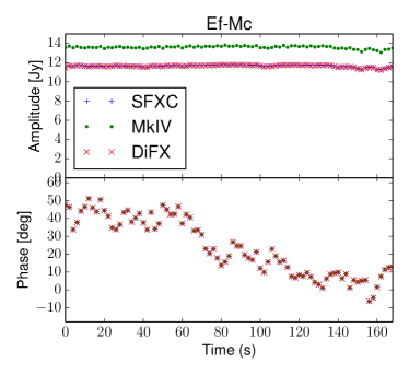
(a) (a)

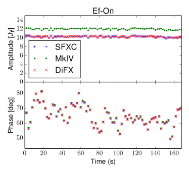
(b) (b)

(c) (c)

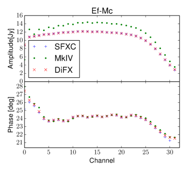
(d) (d)

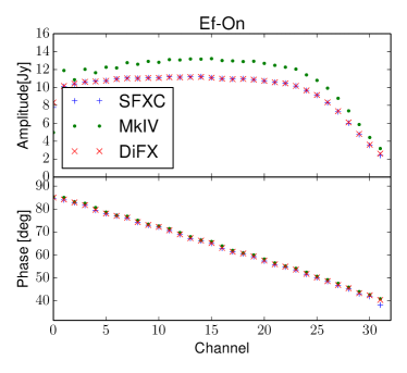
(e) (e)

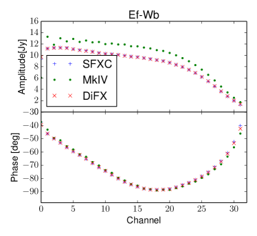
(f) (f)

Figure 7: Comparison of visibility phase and amplitude between SFXC, DiFX, and the EVN MkIV data processor at JIVE for baselines from Effelsberg(Ef) to Medicina(Mc), Onsala(On), and Westerbork(Wb). For details about the observation we refer to the main text. (a)-(c) Amplitude and phase as a function of time, averaging in frequency over the inner 80% of the band. (d)-(f) Amplitude and phase as a function frequency, averaging in time over 170 seconds.

In this section we give a brief comparison between SFXC, DiFX, and the EVN MkIV data processor at JIVE. To this end we correlated an observation of quasar 4C39.25 at 6 cm wavelength using these three correlators. The observation was performed using 8 MHz sub-bands and dual circular polarizations. The data was quantized using two bit sampling and was recorded in the mark4 data format, which all three correlators can read natively.

By default DiFX uses a different delay model than SFXC and the EVN MkIV data processor at JIVE. To make a direct comparison of visibility phases possible we overrode the default delay model in DiFX and used the same CALC 10 delay model with all three correlators.

As was noted in Sec. 5.4, SFXC and the MkIV data processor share the same post- correlation toolchain (Campbell, 2008), which applies a number of corrections to the data. For SFXC only a quantization loss correction is applied to the data. The fact that the input signal is quantized using a finite number of bits leads to a lowering of visibility amplitudes (Thompson et al, 2001, Sec 8.3). For ideally quantized two bit data this effect leads to a reduction in amplitude by 12%. There are a number of additional corrections that are applied to the data produced by the MkIV data processor, which compensate for various approximations that are made in the MkIV data processor’s correlation algorithm (Campbell, 2008). These corrections scale visibility amplitudes by an additional 22%.

The data was correlated using 32 spectral points per sub-band, and a 2 second integration time. The raw correlated data was converted to FITS-IDI and loaded into the data reduction package AIPS . Using the AIPS task ACCOR a quantization loss correction was applied to the DiFX data. As was noted previously, both SFXC and the MkIV already had this correction applied to their data.

In Fig. 7 we show visibility phase and amplitude for a number of baselines. The visibility phases from the three correlators agree to a fraction of a degree of phase with each other. Unfortunately, the EVN MkIV data processor at JIVE suffered from known amplitude scaling issues. In Tab. 2 we show the ratios between the visibility amplitudes from the three correlators. While the amplitudes from both SFXC and DiFX agree very closely, the amplitudes from the MkIV data processor are on average 17% higher than the other two correlators. Similar amplitude scaling issues were reported for the MkIV correlator at Haystack observatory Capallo (2011). It should be emphasized that these higher correlation amplitudes are purely a scaling issue and do not correspond to a higher signal to noise.

Baseline	SFXC / MkIV	SFXC / DiFX	DiFX / MkIV
Ef-Mc	0.857	1.002	0.856
Ef-On	0.856	1.000	0.856
Ef-Wb	0.849	1.002	0.847

Table 2: Visibility amplitude ratios for the data shown in Fig. 7.

7 Performance

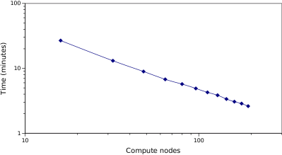
(a) (a)

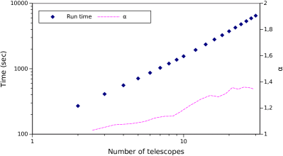
(b) (b)

Figure 8: (a) Correlation time as a function of the number of correlator nodes, (b) Correlation time $T$ as a function of the number of telescopes $N_{t}$ together with the exponential growth factor $\alpha$ which is computed by fitting the relation $T=CN_{t}^{\alpha}$ to consecutive data points, where $C$ is a constant.

In this section we present a number of benchmarks performed on the EVN software correlator cluster at JIVE. The cluster consists (2014) of 40 nodes all of which are equipped with two Intel Xeon processors, yielding a total of 384 CPU cores. The cluster nodes are interconnected via QDR Infiniband, while each node is connected to the outside world via two bonded gigabit Ethernet links. In addition a number of nodes are equipped with 10 Gb/s Ethernet interfaces to accommodate e-VLBI. Currently the cluster is capable of processing 14 stations at 1 Gb/s datarate in real-time.

When available, SFXC will utilise the Intel Performance Primitives (IPP) library. This library provides vectorized math routines for array manipulation utilizing the SIMD instructions available in modern Intel-compatible CPU’s. Furthermore, the library includes highly optimized FFT routines. If the IPP library is not present SFXC will fall back on the FFTW3 (Frigo and Johnson, 2005) FFT library and uses its own non-SIMD routines for array manipulation. Benchmarks on recent Intel Xeon processors show a performance gain of typically 40% using the IPP libraries. The SFXC installed on the EVN software correlator cluster at JIVE makes use of the IPP libraries.

Software correlation is a data intensive, embarrassingly parallel process and therefore highly scalable. Performance often is determined by the rate at which data can be supplied to the correlator nodes. As we discussed in Sec. 5.2 the input nodes perform a highly CPU-intensive corner turning task. Therefore care should be taken that sufficient resources are available to the input nodes.

Provided that enough IO capacity is available, the performance of the correlator scales linearly with the number of CPU cores. This is illustrated in Fig. 8-(a) where we show the correlation time as a function of the number of correlator nodes. The test was performed on 10 minutes of data recorded at 512 Mb/s with 10 telescopes.

Computational cost in terms of the number of telescopes can be divided into two regimes. In the first regime antenna-based operations, such as delay compensation, dominate. In this regime the correlation time increases approximately linearly with the number of telescopes. In the second regime baseline-based operations dominate, and there the correlation time increases quadratically with the number of telescope. Two kinds of baseline-based operations have to be performed, namely cross-correlations and phase shifts during multiple phase centre correlations. Because these phase shifts are applied relatively infrequently, the cross-correlations dominate the processing. In Fig. 8-(b) we show correlation time as a function of the number of telescopes. The test was done using 20 minutes of data at 512 Mb/s. The number of correlator nodes was limited to 32 which prevents the computation becoming IO limited at the lower bound. As can be seen, the relation between correlation time and the number of telescopes only very slowly departs from linearity, and even for 30 telescopes the growth factor is still below 1.5.

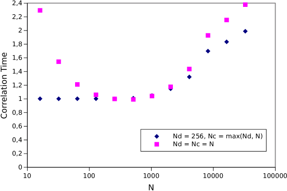
Figure 9: Correlation time as a function of the number of spectral points in the output data $N$ for two configurations of the number of frequency points in the delay compensations $N_{d}$ and the number of points in the correlation $N_{c}$. The configuration signalled by the blue diamonds is the SFXC default.

As we described in Sec. 2 the number of spectral points in the delay compensation $N_{d}$ and the number of spectral points in the cross-correlations $N_{c}$ are independent of each other. In Fig.9 we show the correlation time as a function of $N_{c}$ for the case when $N_{c}=N_{d}$, and for the case when $N_{d}=256$ for all $N_{c}$, the latter case being the default. This benchmark shows that the optimum $N_{d}$ equals $256$ or $512$ for our computing hardware. Both $N_{c}$ and $N_{d}$ are user configurable but are not mandatory for the user to specify. When the user requests $N$ spectral points in the output data the following defaults for $N_{d}$ and $N_{c}$ will be chosen:

• When $N\leq 256$, both $N_{d}$ and $N_{c}$ are set to 256. The correlation products are averaged down to $N$ points after integration.

• When $N>256$, $N_{d}$ is set to 256, and $N_{c}$ is equal to $N$.

8 Conclusions and discussion

During the past years the SFXC software correlator has been deployed as the operational EVN correlator at JIVE. As such it has proven to be a highly reliable and stable platform.

We argue that software correlators in general have a number of important advantages over their hardware counterparts. Software is very flexible and easily modified, making it possible to add new functionality with much less effort. This is exemplified by the ever-increasing set of capabilities in SFXC, such as arbitrary spectral resolution, spectral windowing, pulsar binning and gating, including (in)coherent de-dispersion, and correlation with multiple simultaneous phase centres. None of these features were available on the MkIV correlator, nor would they have been straightforward (if at all possible) to implement. This demonstrates how the implementation of a software correlator has brought new science capabilities to the EVN.

Another advantage is that software correlators are far more flexible with respect to their input parameters, while hardware correlators as a rule impose hard limits on parameters such as number of spectral points or number of input stations. Once built, it is nearly impossible to increase the size of a hardware correlator, as most components are custom-made and produced in limited quantities. On the other hand, as shown in Sec. 6, the performance of SFXC scales very well with the available computing resources. As a consequence it is nearly trivial to increase the capacity of a software correlator, only involving the purchase of additional off-the-shelf hardware. And as a result of Moore’s law, these additions will be more powerful and consume less power, at a lower price.