Introduction to Holographic Superconductor Models
Abstract
In the last years it has been shown that some properties of strongly coupled superconductors can be potentially described by classical general relativity living in one higher dimension, which is known as holographic superconductors. This paper gives a quick and introductory overview of some holographic superconductor models with s-wave, p-wave and d-wave orders in the literature from point of view of bottom-up, and summarizes some basic properties of these holographic models in various regimes. The competition and coexistence of these superconductivity orders are also studied in these superconductor models.
CCTP-2015-06
CCQCN-2015-65
1 Introduction
The phenomenon of superconductivity was discovered in the early part of the last century that the electrical resistivity of a material suddenly drops to zero below a critical temperature . More importantly, the so-called Meissner effect tells us that the magnetic field is expelled in the superconducting phase, which is distinguished from the perfect conductivity. In the latter case a pre-existing magnetic field will be trapped inside the sample. Conventional superconductors are well described by BCS theory [1], where the condensate is a Cooper pair of electrons bounded together by phonons. According to the symmetry of the spatial part of wave function of the Cooper pair, superconductors can be classified as the s-wave, p-wave, d-wave, f-wave superconductors, etc. However, some materials of significant theoretical and practical interest, such as high temperature cuprates and heavy fermion compounds, are beyond BCS theory. There are indications that the involving physics is in strongly coupled regime, so one needs a departure from the quasi-particle paradigm of Fermi liquid theory [2]. Condensed matter theories have very few tools to do this.
On the other hand, although some of the deeper questions arising from the Anti-de Sitter/Conformal Field Theory(AdS/CFT) correspondence [3, 4, 5] remain to be understood from first principles, this duality creating an interface between gravitational theory and dynamics of quantum field theory provides an invaluable source of physical intuition as well as computational power. In particular, in a “large and large ” limit, the gravity side can be well described by classical general relativity, while the dual field theory involves the dynamics with strong interaction.555Loosely speaking, can be considered as the degrees of freedom in the dual field theory, and as the characteristic strength of interactions. An elementary introduction to this correspondence can be found in the next section. It is often referred to as “holography” since a higher dimensional gravity system is described by a lower dimensional field theory without gravity, which is very reminiscent of an optical hologram. There are indeed many physical motivations that lead to this amazing holographic duality in the literature, such as renomalization group flow and black hole membrane paradigm. A very new perspective was proposed, which is called the exact holographic mapping [6]. By constructing a unitary mapping from the Hilbert space of a lattice system in flat space (boundary) to that of another lattice system in one higher dimension (bulk), it provides a more explicit and complete understanding of the bulk theory for a given boundary theory and can be compared with AdS/CFT correspondence.
It has been shown that the AdS/CFT correspondence can indeed provide solvable models of strong coupling superconductivity, see refs. [7, 8, 9, 10] for reviews. The physical picture is that some gravity background would become unstable as one tunes some parameter, such as temperature for black hole and chemical potential for AdS soliton, to developing some kind of hair. The emergency of the hair in the bulk corresponds to the condensation of a composite charged operator in the dual field theory. More precisely, the dual operator acquires a non-vanishing vacuum expectation value breaking the U(1) symmetry spontaneously. It has been uncovered that this simple holographic setup shows similar properties with real superconductors.
The holographic s-wave superconductor model known as Abelian-Higgs model was first realized in refs. [11, 12]. According to the AdS/CFT correspondence, in the gravity side, a Maxwell field and a charged scalar field are introduced to describe the U(1) symmetry and the scalar operator in the dual field theory, respectively. This holographic model undergoes a phase transition from black hole with no hair (normal phase/conductor phase) to the case with scalar hair at low temperatures (superconducting phase). The holographic model for the insulator/superconductor phase transition has been realized in ref. [13] at zero temperature by taking the AdS soliton as the gravitational background in the Abelian-Higgs model. Holographic d-wave model was constructed by introducing a charged massive spin two field propagating in the bulk [14, 15]. The superconductivity in the high temperature cuprates is well known to be of d-wave type.
In recent years, evidence from several materials suggests that we now have examples of p-wave superconductivity, providing us new insights into the understanding of unconventional superconductivity in strongly correlated electron systems [16]. To realize a holographic p-wave model, one needs to introduce a charged vector field in the bulk as a vector order parameter. Ref. [17] presented a holographic p-wave model by introducing an SU(2) Yang-Mills field into the bulk, where a gauge boson generated by one SU(2) generator is dual to the vector order parameter. The authors of refs. [18, 19] constructed a holographic p-wave model by adopting a complex vector field charged under a U(1) gauge field, which is dual to a strongly coupled system involving a charged vector operator with a global U(1) symmetry. An alternative holographic realization of p-wave superconductivity emerges from the condensation of a two-form field in the bulk [20, 21, 22].
The philosophy for holographic setups is that even though the underlying microscopic description of the theory with a gravity dual is quite likely to be different form that arising in materials of experimental interest, it may uncover some universal aspects of the strongly coupled dynamics and kinematics, thus would help the development of new theories of superconductivity. By mapping the quantum physics of strongly correlated many body systems to the classical dynamics of black hole physics in one higher dimension, the holographic approach provides explicit examples of theories without a quasi-particle picture in which computations are nevertheless feasible.
The models studied in the literature can be roughly divided into two classes, i.e., the bottom-up and top-down models. In the former approach the holographic model is constructed phenomenologically by picking relevant bulk fields corresponding to the most important operators on the dual field theory and then writing down a natural bulk action considering general symmetries and other features of dual system. Thus the holographic description is necessarily effective and can be used to describe a wide class of dual theories instead of a definite single theory. In the top-down approach, the construction of a model is uniquely determined by a consistent truncation from string theory or supergravity. One can usually have a much better control over the dual field theory, nonetheless, the resulted models are much more complicated.
This paper aims at providing a quick and introductory overview of those three kinds of holographic superconductor models from the point of view of bottom-up.666Holographic superconductor models constructed in the top-down approach can be found, for example, in refs. [23, 24, 25, 26, 27, 28, 29]. The organization of the paper is as follows. In the next section, we review basic elements of Ginzburg-Landau theory of superconductivity and holographic duality, as a warm up. A brief introduction to the Abelian-Higgs model is presented in section 3. In section 4, we first introduce the SU(2) Yang-Mill model, focusing on its condensate and conductivity, then study the Maxwell-vector model, paying more attention to the vector condensate induced by magnetic fields and its complete phase diagram in terms of temperature and chemical potential, and finally discuss the third p-wave model by introducing a two-form in the bulk. This model can exhibit a novel helical superconducting phase. Section 5 is devoted to holographic d-wave models. In the next two sections, we pay attention to the competition and coexistence among different orders, including different superconducting orders in section 6 as well as superconducting order and magnetic order in section 7. The conclusion and some discussions are included in section 8.
2 Preliminary
2.1 Ginzburg-Landau theory
The microscopic origin of traditional superconductivity is well understood by BCS theory, which explained the superconducting current as a superfluid of pairs of electrons interacting through the exchange of phonons. However, at phenomenological level, the Ginzburg-Landau theory of superconductivity [30] had great success in explaining the macroscopic properties of superconductors. 777To have a wide description of the Ginzburg-Landau theory see ref. [31] and references therein.
In this phenomenological theory, the free energy of a superconductor can be expressed in terms of a complex order parameter field, , which is directly related to the density of the superconducting component. By assuming smallness of and smallness of its gradients, the free energy near the superconducting critical temperature has the following form,
| (1) |
where is the free energy in the normal phase, is the vector potential and is the magnetic field. and are effective mass and charge of condensate. If one considers the BCS theory, and with and the mass and charge of electrons forming Copper pairs. and are two phenomenological parameters, which behave as with and two positive constants. Note that we work in the unites . It is obvious that the free energy is invariant under the following transformation,
| (2) |
which is known as the U(1) gauge symmetry.
Minimising the free energy with respect to the order parameter and the vector potential, one obtains the Ginzburg-Landau equations,
| (3) | |||
| (4) |
The first equation determines the order parameter , and the second one provides the superconducting current which is the dissipation-less electrical current. The Ginzburg-Landau theory actually can be derived from the BCS microscopic theory. Thus, the electrons that contribute to superconductivity would form a superfluid and indicates the fraction of electrons condensed into a superfluid.
This phenomenological theory can give many useful information even in homogeneous case. Let us consider a homogeneous superconductor with no superconducting current, so the equation for simplifies to
| (5) |
Above the superconducting transition temperature, , one only gets a trivial solution , which corresponds to the normal state of the superconductor. Below the critical temperature, , apart from the trivial solution, there are a series of non-trivial solutions which read
| (6) |
Furthermore, compared with , those solutions have lower potential energy, thus are dominant. Note that there are infinite solutions giving the ground state of superconducting phase. However, the true ground state can only choose one solution from them. Therefore, the ground state will change under the U(1) transformation (2). In such case, we call that the U(1) symmetry is spontaneously broken. From (6) one sees that approaches zero as gets closer to from below, which is a typical behaviour of a second order phase transition. One can find from (4) that in the homogeneous case one can neglect the contribution from the first term and thus the superconducting current is proportional to the vector potential, i.e., . If one takes a time derivative on both sides, one will obtain . This means that the electric fields accelerate superconducting electrons resulting in the infinite DC conductivity. If one takes the curl and combines with Maxwell’s equations, one will find indicating the decay of magnetic fields inside a superconductor, i.e., the Meissner effect.
The Ginzburg-Landau equations predict two characteristic lengths in a superconductor. The first one is the coherence length which is given by
| (7) |
It is the characteristic exponent of the variations of the density of superconducting component. In the BCS theory denotes the characteristic Cooper pair size. The other one is the penetration length which reads
| (8) |
where is the equilibrium value of the order parameter in the absence of electromagnetic fields. This length characterises the speed of exponential decay of the magnetic field at the surface of a superconductor.
Note that from definitions (7) and (8) the temperature dependences near behave as
| (9) | |||||
| (10) |
Both diverge as from below with the critical exponent . Nevertheless, the ratio known as the Ginzburg-Landau parameter is temperature independent. Type-I superconductors correspond to cases with , and type-II superconductors correspond to cases with . One of the most important findings from the Ginzburg-Landau theory was that in a type-II superconductor, strong enough magnetic fields can penetrate the superconductor by forming the hexagonal lattice of quantised tubes of flux, called the Abrikosov vortex lattice.
Finally one point we would like to emphasize is that in the Ginzburg-Landau theory the U(1) symmetry is broken spontaneously in the superconducting phase transition. Actually, only the spontaneous symmetry breaking feature itself can lead to many fundamental phenomenological properties of superconductivity, without any precise detail of the breaking mechanism specified [32]. In this review, we will show how a similar effective approach constitutes the basis of superconductivity in terms of holographic description.
2.2 Holographic duality
The original conjecture proposed by Maldacena [3] was that type-IIB string theory on the product spacetime should be equivalent to SU(N) supersymmetric Yang-Mills theory on the 3+1 dimensional boundary. This super-Yang-Mills theory is a conformal field theory, so this duality is named AdS/CFT correspondence. Later, this conjecture has been generalized to more general gravitational backgrounds and cases without supersymmetry and conformal symmetry.888The simple examples are Lifshitz symmetry [33] and Schrödinger symmetry [34, 35], while more generic cases are those with generalized Lifshitz invariance and hyperscaling violation [36, 37, 38, 39], and the associated Schrödinger cousins [40]. However, those take us outside the best understood AdS/CFT framework. We shall focus on the most well defined case involving the bulk geometry with the asymptotically AdS behaviour. From a modern perspective, the correspondence is an equality between a quantum field theory (QFT) in d dimensional spacetime and a (quantum) gravity theory in d+1 spacetime dimensions. This correspondence is also sometimes called gauge/gravity duality, gauge/string duality or holographic correspondence (or duality).
A remarkable usefulness of the correspondence comes from the fact that it is a strong-weak duality: when the quantum field theory is strongly coupled, the dual gravitational theory is in a weakly interacting regime and thus more mathematically tractable, and vice versa. So the holographic duality provides us a powerful toolkit for studying strongly interacting systems. The backbone of the correspondence was elaborated by the authors of refs. [4, 5]. For every gauge invariant operator in the QFT, there is a corresponding dynamical field in the bulk gravitational theory. The partition function in gravity side is equal to the generating functional of the dual boundary field theory. More specifically, adding a source for in the QFT is equivalent to impose a boundary condition for the dual field at the boundary of the gravity manifold (say at ), i.e., the field tends towards the value at the boundary up to an overall power of . The formula reads
| (11) |
where is the determinant of the background metric of dual field theory. If we want to study a strongly coupled field theory, we can translate it into a weakly coupled gravity system. In the semiclassical limit, the partition function is equal to the on-shell action of the bulk theory and thus one only needs to solve particular differential equations of motion. Therefore we can compute expectation values and correlation functions of the operator in the (strongly coupled) QFT by differentiating the left side with respect to .
In order to get familiar with the calculation by holography, let us consider as a scalar operator which is dual to the bulk scalar field also denoted as . The minimal bulk action for is given by
| (12) |
For illustration the gravity background is fixed as the pure in Poincáre coordinates
| (13) |
together with a profile for the scalar field . Here are spatial coordinates, is a timelike coordinate and is the radial spatial coordinate. is known as AdS radius and the conformal boundary of AdS is located at . Note that the geometry is invariant under the scaling transformation . Actually, the full isometry group of is identical to the conformal group in d dimensional boundary spacetime.
To calculate the on-shell action for , we need to solve the equation of motion derived from action (12). Working in Fourier space , we obtain
| (14) |
Near the boundary , the above equation admits the general asymptotic solution,
| (15) |
with .999Note that spacetime is stable even when the mass squared of scalar field is negative provided [41]. The lower bound is often called Breitenloner-Freedman (BF) bound. The relation between A and B is determined by the interior of AdS. Making Fourier transformation back into real space, we then obtain
| (16) |
We now try to identify which term can be considered as the source of the dual operator . It turns out that, as long as , the mode is non-normalizable with respect to the inner product
| (17) |
with a constant- slice. The mode in this case is normalizable. We identify the coefficient as the source term, i.e.,
| (18) |
This means that the on-shell action, and thus the partition function in AdS is a functional of . We can now argue that the scaling dimension of is without further calculation. Consider the scale transformation , the scalar under such operation transforms as . So the source term must transform as , and thus according to (11) transforms as which suggests the dimension of should be .
Calculating the on-shell bulk action in terms of the solution with asymptotic expansion (16), one will find that the on-shell action will diverge near the boundary . This divergence is interpreted as dual to UV divergences of the boundary field theory. Actually, the infrared (IR) physics of the bulk near the boundary corresponds to the ultraviolet (UV) physics of dual QFT, and vice versa. This is called UV/IR relation [42] and the radial direction plays the role of energy scale in the dual boundary theory. Physical processes in the bulk occurring at different radial positions correspond to different field theory processed with energies which scale as .
The divergence can be cured by adding local counter terms at the boundary, known as holographic renormalization [43, 44, 45]. For the present case the counter term to be introduced is
| (19) |
where is the determinant of the induced metric at the boundary. So the renormalized on-shell action should be . We can then compute the expectation value by using the basic formula (11). That relation implies
| (20) |
where we have taken the semiclassical limit . Straightforward calculation shows that
| (21) |
This is often summarised as saying that the “non-normalizable” mode gives the source in the dual field theory, whereas the “normalizable” mode encodes the response.
In the real world, many important experimental processes such as transport and spectroscopy involve small time dependent perturbations about equilibrium. Those phenomena can be described by linear response theory, in which the basic quantity is the retarded Green’s function. The retarded Green’s function is defined to linearly relate sources and corresponding expectation values. In frequency space, it can be written as
| (22) |
Using above formula one can continue to compute which is given by
| (23) |
However, there is something subtle we shall discuss here. Different from the case in Euclidean signature where the bulk solution can be uniquely determined by additional requirement of regularity in the IR, while in the real-time Lorentzian signature, we must choose an appropriate boundary condition in far IR region of the geometry. This ambiguity reflects multitude of real-time Green’s functions (Feynman, retarded, advanced) in the QFT. Since the retarded Green’s function describes causal response of the system to a perturbation, we involve an in-going condition describing stuff falling into the IR, i.e., moving towards larger as time passes. The advanced Green’s function corresponds to the choice of out-going condition enforced in the IR region. 101010An intrinsically real-time holographic prescription was first proposed by the authors of ref. [46] by essentially analytically continuing the Euclidean prescription. It has been justified by a holographic version of the Schwinger-Keldysh formalism [47, 48].
Let us briefly consider the case with where the second restriction comes from the unitary bound. One can easily check that both terms in (16) are normalizable with the inner product (17). So either one can be considered as a source, and the other one as a response. These two ways to quantize a scalar field in the bulk by imposing Dirichlet or Neumann like boundary conditions correspond to two different dual field theories [49], respectively. In the standard quantization, the corresponding operator has dimension , while in the alternative quantization, the corresponding operator has dimension . 111111In fact, it has been shown that even more general quantisations are possible, like double trace deformation, see, for example, refs. [50, 51].
The above discussion only uses the near boundary expansion (16) and thus applies to generic asymptotically AdS geometries. It can also be applied to other fields such as components of the metric and Maxwell fields. To sum up, we first obtain a solution which satisfies appropriate boundary conditions, especially the condition in the deep IR. Then we compute the properly renormalized on-shell action, identify the source and response from the asymptotic behaviour of the solution near the boundary, and compute the Green’s function through linear response. In the next section we will use this procedure to compute the optical conductivity.
Another essential entry in the holographic dictionary is that the thermodynamic data of the QFT is entirely encoded in the thermodynamics of the black hole in the dual geometry. QFT states with finite temperature are dual to black hole geometries, where the Hawking temperature of the black hole is identified with the temperature in the QFT. Turning on a chemical potential in this QFT corresponds to gravity with a conserved charge. The thermal entropy of QFT is identified as the area of black hole horizon and the free energy is related to the Euclidian on-shell bulk action. As space is limited, we only introduce essential issues which will be needed to discuss holographic superconductors.
Before the end of this subsection, let us point out that the holographic duality can be used to understand some hard nuts in quantum gravity from dual field theory side. A typical example is the black hole information paradox. It was first suggested by Hawking [52] that black holes destroy information which seemed to conflict with the unitarity postulate of quantum mechanics. The black hole information paradox can be resolved, at least to some extent, by holography, because it shows how a black hole can evolve in a manner consistent with quantum mechanics in some contexts, i.e., evolves in a unitary fashion [53, 54]. There are some excellent papers talking about aspects of holographic duality, see, for example, refs. [55, 56, 57, 58, 59, 60] for more details.
3 Holographic S-wave Models
3.1 The Abelian-Higgs model
In this subsection, we begin with the Abelian-Higgs model [11] by introducing a complex scalar field , with mass and charge , into the dimensional Einstein-Maxwell theory with a negative cosmological constant. The complete action can be written down as 121212The model is a s-wave one since the condensed field is a scalar field dual to a scalar operator in the field theory side. This model can be straightforwardly generalized to other spacetime dimensions. Holographic s-wave superconductors with generalised couplings have also been considered in a number of works [61, 62, 63, 64, 65, 66, 67, 68, 69].
| (24) |
where with being the Newtonian gravitational constant, is the scalar curvature of spacetime, is the AdS radius and Maxwell field strength . If one rescales and , then the matter part has an overall factor in front of its Lagrangian, thus the back reaction of the matter fields on the metric becomes negligible when is large. The limit with and fixed is called the probe limit. Here we will review the results obtained in this probe approximation, which can simplify the problem while retains most of the interesting physics. The study including the back reaction of matter fields can be found in ref. [12].
The background metric is the AdS-Schwarzschild black hole with planar horizon
| (25) |
where we have set the AdS radius to be unity. The conformal boundary is located at . The Hawking temperature of the black hole is determined by the horizon radius : . The solution describes a thermal state of dual field theory in (2+1)-dimensions with temperature . In addition, it is clear that the AdS-Schwarzschild black hole is an exact solution of the action (24) when the matter sector is negligible. It will be seen shortly that when the temperature is lowered enough, the black hole solution will become unstable and a new stable black hole solution appears with nontrivial scalar field.
To see the formation of scalar hair, we are interested in static, translationally invariant solutions, thus we consider the ansatz [11]
| (26) |
The component of Maxwell equations implies that the phase of must be constant. Therefore, for convenience, one can take to be real. This leads to the equations of motion 131313In the probe limit, the concrete value of the charge does not play an essential role. Without loss of generality, we take to be one.
| (27) |
As pointed out in ref. [70], the coupling of the scalar to the Maxwell field produces a negative effective mass for (see the third term in the first equation). Since this term becomes more important at low temperatures, we expect an instability towards forming nontrivial scalar hair.
The asymptotic behaviours of scalar field and gauge field near the AdS boundary are
| (28) |
where , is the chemical potential and is the charge density in the dual field theory. According to the AdS/CFT dictionary, the leading coefficient is regarded as the source of the dual scalar operator with scaling dimension . Since we want the U(1) symmetry to be broken spontaneously, we should turn off the source, i.e., . Therefore the subleading term provides the vacuum expectation value in the absence of any source. 141414We only consider the standard quantization here, regarding the leading coefficient as the source of dual operator. An alternative way inducing spontaneous symmetry breaking in holographic superconductors is to introduce double trace deformation [71].
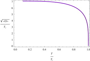
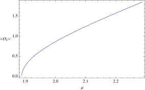
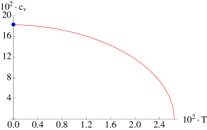
Figure 1 shows how the condensate behaves as a function of temperature in a canonical ensemble with fixed to be one. As one can see that there is a critical temperature below which the condensate appears, then rises quickly as the system is cooled and finally goes to a constant for sufficiently low temperatures. This behaviour is qualitatively similar to that obtained in BCS theory and observed in many materials. Near the critical temperature , , which is the typical result predicated by Ginzburg-Landau theory, see equation (6). By comparing the free energy of these hairy configurations to the solution with no scalar hair, one finds that the hairy phase is thermodynamically favoured and the difference of free energies behaves like near the critical point, indicating a second order phase transition.
We now compute the optical conductivity, i.e., the conductivity as a function of frequency , which is related to the retarded current-current two-point function for the U(1) symmetry, . According to the holographic duality, this can be obtained by calculating electromagnetic fluctuations in the bulk. By symmetry, it is sufficient to turn on the perturbation , then the linearized equation of motion for is
| (29) |
To obtain the real time correlation functions for the dual boundary theory, the holographic description associates in-going and out-going boundary conditions at the black hole horizon to retarded and advanced boundary correlators respectively [46]. To consider causal behaviour, one should impose the in-going wave condition at the horizon: . Near the AdS boundary, the asymptotic behaviour of is given by
| (30) |
According to the AdS/CFT correspondence, is the source, while is dual to the current. Thus one can obtain
| (31) |
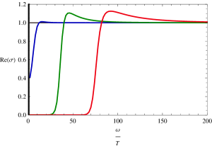
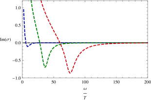
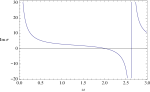
The AC conductivity as a function of frequency is presented in figure 2. Above the critical temperature, the conductivity is a constant. As the temperature is lowered below , the optical conductivity develops a gap at some special frequency known as gap frequency. As suggested in ref. [72], it can be identified with the one at the minimum of the imaginary part of the AC conductivity. Re is very small in the infrared and rises quickly at .151515It has been shown that the conductivity is directly related to the reflection coefficient with the frequency given the incident energy [73]. The key point is that even as there is still tunneling through the barrier provided by the effective potential. Therefore, a nonzero conductivity at small frequencies will always exist, and hence there is no hard gap in the optical conductivity at zero temperature. To obtain a superconductor with a hard gap, one might consider non-minimally coupled scalars in the bulk. There also exists a small “bump” slightly above , which is reminiscent of the behaviour due to fermionic pairing [17]. For different choice of parameters, one can obtain a robust feature with deviations of less than . Compared to the corresponding BCS value , the result shown here is consistent with the fact that the holographic model describes a system at strong coupling. There is also a delta function at appearing as soon as . This can be seen from the imaginary part of the conductivity. According to the Kramers-Kronig relation
| (32) |
one can conclude that the real part of the conductivity contains a Dirac delta function at if and only if the imaginary part has a pole, i.e., Im.
From above discussion, we see that this simple model can provide a holographically dual description of a superconductor. It predicts that a charged condensate emerges below a critical temperature via a second order transition, that the DC conductivity becomes infinite, and that the optical conductivity develops a gap at low frequency. The temperature dependences of the coherence length as well as the penetration length in the holographic model are both proportional to near the critical temperature [72, 74]. It has been shown that this holographic superconductor is type-II [12]. The condensate can form a lattice of vortices and the minimum of the free energy at long wavelength corresponds to a triangular array [75]. The effects of a superconducting condensate on holographic Fermi surfaces have been studied [76, 77]. All these features are very reminiscent of real superconductors. Although the holographic model is very simple, it indeed captures some significant characteristics for superconductivity, thus helping us to understand real, strongly coupled superconductors.
3.2 Holographic insulator/superconductor phase transition
In this subsection, let us consider a five-dimensional Einstein-Abelian-Higgs theory with following action
| (33) |
When one does not include the matter sector, the theory has a five-dimensional AdS-Schwarzschild black hole solution. It is interesting to note that there also exists another exact solution, so-called AdS soliton, in the theory (33). The AdS soliton solution can be obtained by double Wick rotation from the AdS-Schwarzschild black hole as
| (34) |
To remove the potential conical singularity, the spatial coordinate has to be periodic with a period . If one considers the coordinates , the geometry looks like a cigar and the tip is given by . The AdS soliton has no horizon, and therefore no entropy is associated with this solution. Due to the existence of an IR cutoff at for the soliton solution, the field theory dual to this gravity background turns out to be in confined phase at zero temperature. Furthermore, this solution can be explained as a gravity dual to an insulator in condensed matter theory. If one increases the chemical potential to a critical value, the AdS soliton solution becomes unstable to developing a scalar hair with nontrivial scalar profile. It is shown that the new solution can describe a superconducting phase [13]. In this way, the holographic insultor/superconductor phase transition at zero temperature can be realized in the Abelian-Higgs model (33).
More precisely, let us also consider the following ansatz in the probe limit
| (35) |
In the AdS soliton (34) background, the equations of motions turn out to be
| (36) |
In the five-dimensional case, the BF bound is . For simplicity, let us consider the case with . To solve the equations of motion, we have to specify the boundary conditions both at the tip and the AdS boundary. Near the AdS boundary, we have the following asymptotical form
| (37) |
Note that in this case, both terms proportional to and are normalizable, so the corresponding operators and have dimensions and , respectively. On the other hand, near the tip of the soliton, these fields behave like
| (38) |
where and are all constants. The field regularity at the tip requires us to take . As in the previous subsection we can set and further set without loss of generality.
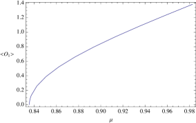
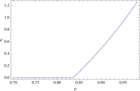
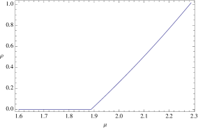
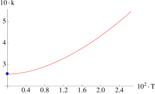
With the boundary conditions, solving the equations of motion, one can find that when the chemical potential is beyond some critical value, the condensation happens. Concretely, for the operator , the critical chemical potential is , while the critical chemical potential for the operator . The behaviour of condensation is plotted in figure 3 with respect to chemical potential. In figure 4 the charge density with respect to chemical potential is plotted. We can see that at the phase transition point, its derivative is discontinuous, which verifies that the phase transition is indeed second order, since one has , where is the Gibbs free energy density.
To calculate conductivity we can consider the perturbation of the component in the soliton background. Assuming it has the form , its equation then turns out to be
| (39) |
At the tip one takes the Newmann boundary condition as in (38). Near the AdS boundary, one has the asymptotical form as
| (40) |
where is a cutoff. The holographic conductivity can be obtained as
| (41) |
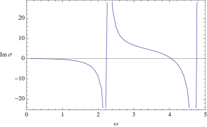
Since the background has no horizon, the real part of the conductivity always vanishes. This means that there is no dissipation. The imaginary part is plotted in figure 5: The left plot corresponds to the case of pure AdS solution without scalar hair, while the right one to the case with nontrivial scalar hair. There exist poles periodically at the points where vanishes. These correspond to normalized modes dual to vector operators. One can see that when is large, both case are similar, while when , they are quite different. In the case without condensation, the imaginary part goes to zero when , while it diverges in the case with condensation. According to the Kramers-Kronig relation (32), it shows that there is a delta functional support for the real part of conductivity at . Therefore the AdS soliton background with nontrivial scalar hair should be identified with the superconductivity.
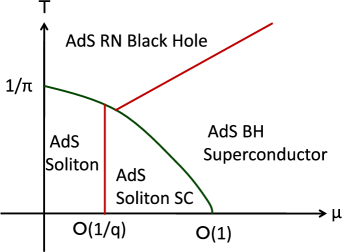
In the Einstein-Abelian-Higgs theory (33), besides the two phases described above, as in the four dimensional case, there exist another two solutions: AdS Reissner Nordström (AdS RN) black hole161616Its precise form can be found in (65) below. without scalar hair and AdS RN black hole with scalar hair, the latter can be identified with a superconductivity phase, while the former is dual to a conductor phase. Combining the four phases together, one could have the phase digram of the theory, which is schematically plotted in figure 6. The green line in the figure denotes the first order phase transition, while two red lines represent second order phase transition. Considering back reaction of matter sector, the complete phase diagrams in terms of temperature and chemical potential for the Abelian-Higgs model have been constructed in ref. [78]. It is interesting to note that the behaviour of the entanglement entropy with respect to chemical potential is non-monotonic and seems to be universal in this kind of insulator/superconductor models [79, 80, 81].
4 Holographic P-wave Models
4.1 The SU(2) Yang-Mills P-wave model
The first holographic p-wave model is constructed by introducing a SU(2) Yang-Mills field in asymptotically AdS spacetime. One of three U(1) subgroups is regarded as the gauge group of electromagnetism and the off-diagonal gauge bosons which are charged under this U(1) gauge field are supposed to condense outside the horizon. The full action is given by [17]
| (42) |
where is the four dimensional gravitational constant, is the Yang-Mills coupling constant and is the AdS radius. The field strength for the SU(2) gauge field is
| (43) |
where denote the indices of spacetime and are the indices of the SU(2) group generators ( are Pauli matrices). is the totally antisymmetric tensor with .
Note that the ratio measures the influence of Yang-Mills field on the background geometry. For the case with fixed, the back reaction of the matter field can be ignored, thus the metric is simply Schwarzschild black hole
| (44) |
with the temperature given by . Without loss of generality, we shall choose , and we also fix a scale by setting .
4.1.1 Vector condensate
To realize the p-wave condensate, one takes the ansatz
| (45) |
It is clear that the non-trivial profile of picks out the direction as special, thus the condensed phase breaks the gauge group generated by and rotational symmetry in plane. The relevant equations are [17]
| (46) |
with primes representing the derivative with respect to .
The regularity at the horizon demands the behaviour like
| (47) |
while the asymptotical expansion near the boundary takes the form
| (48) |
According to the holographic dictionary, is regarded as chemical potential and is the total charged density, and is the source of the dual operator . To spontaneously break the U(1) symmetry, we should impose , then the coefficient gives the vacuum expectation value of . According to the two-fluid model, the total charge density can be divided into two components , where is the normal component, while is the superconducting component. In the holographic setup, the normal charge density is proportional to the part of the electric field at the horizon, i.e., . Therefore the superconducting charge density is .
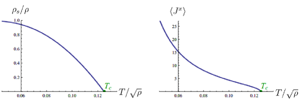
By numerically solving the equations (46), one finds that the condensate is non-vanishing only when the rescaled temperature is small enough, i.e., lower than at which the condensate first turns on. As one can see in the right plot of figure 7, as the temperature is lowered, increases continuously. Near , vanishes as , which is the typical behaviour predicted by Ginzburg-Landau theory. The fraction of the charge carried by the superconducting condensate goes to zero linearly near . 171717The ration versus temperature in the left plot is reminiscent of the temperature dependence of the superfluid of liquid He II as measured from in the torsional oscillation disk stack experiment. However, we find goes to zero linearly here, while the experiment gives a critical exponent about .
We have interpreted generated by as the gauge group of electromagnetism. The condensate of spontaneously breaks this U(1) symmetry as well as the rotational symmetry, thus resulting in an anisotropic superconducting phase. To see this much more clearly, we shall calculate the optical conductivity, which can be deduced by the retarded Green’s function of the current. Similar to the previous section, in gravity side the linear response to electromagnetic probes is turned out to study how linear perturbations of the component of the gauge field propagate.
4.1.2 Conductivity
In the presence of the condensate , the direction is special, so the conductivity along the direction is expected to be different from along the direction. To obtain consistent linearized equations, we can turn on the perturbation [17]
| (49) |
where all the functions depend on only. By plugging the perturbation (49) into the linearized Yang-Mills equation, one finally obtains four second order equations
| (50) |
| (51a) | |||
| (51b) | |||
| (51c) | |||
and two first order constraint equations
| (52) |
It is clear that the equation of motion of the mode decouples from the others, and the conductivity exhibits similar “soft gap” behaviour to the s-wave model [11].181818However, by considering the back reaction to the metric in the SU(2) model (42), it has been shown that the conductivity in the direction has a “hard gap” at zero temperature, i.e., the real part of the conductivity is zero for an excitation frequency less than the gap frequency [82]. What we are interested in is the conductivity in the direction. The conductivity can be determined by solving the coupled equations (51) with the constraints given by (52). More precisely, we impose the ingoing wave condition at the horizon, which corresponds to a retarded Green’s function,
| (53) |
where all the coefficients can be fixed once , and are specified. Near the conformal boundary , one has a generic solution to the equations of motion
| (54) |
As pointed out in ref. [17], there exists a residual gauge invariance. After fixing this residual gauge freedom, one can finally obtain the gauge invariant conductivity along direction
| (55) |
Numerical calculation can only display the continuous part of . One can reveal the non-analytic behaviour by virtue of the Kramers-Krong relations, which tells us that a simple pole in at implies a delta function to . Further more, the positivity constraint on the real part of conductivities requires any pole of on the real axis to have a positive residue.
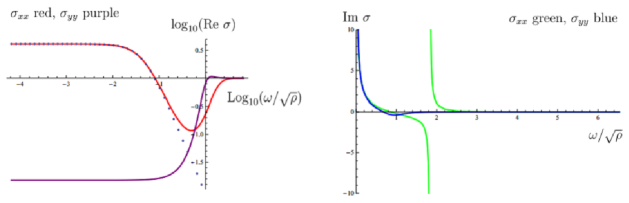
The behaviour of conductivities as a function of frequency is shown in figure 8, from which one can see the following features [17]. First, both and approach constant for sufficiently large . This is because the condensate involves dynamics with a characteristic energy scale set by . If , the propagation of the gauge boson should become insensitive to the condensate and can be approximated by the case in pure , thus is a constant. Second, exhibits gapped dependence similar to the Abelian-Higgs model in figure 2. is very small in the infrared, then rises quickly at . There is a slight “bump” a little above which is reminiscent of the behaviour expected for fermionic pairing. Third, there is a pole in at . Therefore, there is a delta function contribution to at . Finally, in the small region, can be well parameterized in terms of the Drude model
| (56) |
where gives the DC conductivity and is the scattering time. The best fit gives a narrow Drude peak in and suggests conductivity due to quasi-particles with scattering time to diverge as .
We do not have a microscopic description of the condensate in the language of the dual theory without gravity. However, we know clearly that there is an SU(2) current algebra, and the component develops an expectation for sufficiently large chemical potential. Yet we only turn on mode corresponding to the p-wave background. The -wave case can be realized by involving the combination . This mode results in an isotropic superconducting phase which exhibits a pseudogap191919The terminology “pseudogap” here is to denote a well defined gap in the dissipative conductivity at low frequencies in which the conductivity is not identically zero. at low temperatures and a nonzero Hall conductivity with no external magnetic field [83]. However, it should be pointed out that configurations are unstable against turning into pure p-wave background. The insulator/superconductor phase transition for the SU(2) p-wave model has been studied in ref. [84].
A new ground state can be found when a magnetic component of the gauge field is larger than a critical value, which forms a triangular Abrikosov lattice in the spatial directions perpendicular to the magnetic field [85, 86]. In the same spirit, a p-wave superconductor for which the dual field is explicitly known has been constructed in refs. [87, 88, 89] by embedding a probe of two coincident D7-branes in the AdS black hole background. From this top-down approach one can try to identify the SU(2) chemical potential as an isospin chemical potential and the condensate as a meson. The back reaction of the gauge field on the metric in the SU(2) Yang-Mills model has been considered in refs. [90]. It is interesting to note that when the back reaction is strong enough, the phase transition will be a first order one. The holographic SU(2) p-wave superconductor model has been extended to include, for example, the Gauss-Bonnet term [91, 92] and Chern-Simons coupling [93]. In addition, based on the backreacted metric, the behaviour of entanglement entropy in the holographic superconducting phase transitions has been studied in refs. [94, 95, 96].
4.2 The Maxwell-Vector P-wave model
Let us introduce a charged vector field into the dimensional Einstein-Maxwell theory with a negative cosmological constant. The full action reads [18, 19]
| (57) |
where a dagger denotes complex conjugation and is a complex vector field with mass and charge . We define with the covariant derivative . The last non-minimal coupling term characterizes the magnetic moment of the vector field .
Since is charged under the U(1) gauge field, according to AdS/CFT correspondence, its dual operator will carry the same charge under this symmetry and a vacuum expectation value of this operator will then trigger the U(1) symmetry breaking spontaneously. Thus, the condensate of the dual vector operator will break the U(1) symmetry as well as the spatial rotational symmetry since the condensate will pick out one direction as special. Therefore, viewing this vector field as an order parameter, the holographic model can be used to mimic a p-wave superconductor (superfluid) phase transition. The gravity background without vector hair ()/with vector hair () is used to mimic the normal phase/superconducting phase in the dual system.
Indeed, it was shown in ref. [18] that working on the probe limit, as one lowers the temperature, the normal phase becomes unstable to developing nontrivial configuration of the vector field. The calculation of the optical conductivity reveals that there is a delta function at the origin for the real part of the conductivity, which means the condensed phase is indeed superconducting. In this subsection, we shall review the effect of a background magnetic field on the model and its complete phase diagram in terms of temperature and chemical potential.
4.2.1 Condensate induced by magnetic field
Generally speaking, to consider the case with a magnetic field, one needs to solve coupled partial differential equations which is much more involved in practice. However, if one is interested in the instability induced by the magnetic field, one can overcome this difficulty by only focusing the dynamics near the critical point at which the condensate is very small. More precisely, one can introduce a deviation parameter from the critical point at which the condensate begins to appear. The coupled equations of motion can then be solved order by order in terms of the power of .
Following the above procedure, we now turn on a magnetic field to study how the applied magnetic field influences the system. The background is taken to be a (3+1) dimensional AdS-Schwarzschild black hole (25). A consistent ansatz is as follows [18]
| (58) |
where , are all real functions, is a real constant and the constant is the phase difference between the and components of the vector field . The constant magnetic field is perpendicular to the plane.
The profile of can be uniquely determined at the zeroth order of , which takes the form
| (59) |
with interpreted as the chemical potential. The equations of motion for and can be deduced from (57) at order . We further separate the variables as and . Then one can get the following equations 202020 In order to satisfy the equations of motion with the given ansatz, can only be chosen as or with an arbitrary integer. Here and below the upper signs correspond to the case and the lower to the case.
| (60) |
where the prime denotes the derivative with respect to and the dot denotes the derivative with respect to . We have also made a consistent assumption and is a constant coming from variables separation. The last two equations for and can be solved analytically and the eigenvalue is given by where can be chosen as a non-negative integer.
We are interested in how the applied magnetic field influences on the transition temperature from the normal phase to the condensed phase. The effective mass of the charged vector field in the lowest energy state, i.e., in the lowest Landau level depends on the magnetic field and the non-minimal coupling parameter as
| (61) |
It is clear that the increase of the magnetic field decreases the effective mass and thus tends to raise the transition temperature, even in the case that the electric field is turned off. Only the magnetic field itself can trigger the phase transition. This result has an analogy to the QCD vacuum instability induced by a strong magnetic field to spontaneously developing the -meson condensate. It is clear that the last term in (57) describing a non-minimal coupling of the vector field to the gauge field plays a crucial role in the instability. Note that similar coupling can be found in many formalisms used to describe the coupling of magnetic moment to the background magnetic field for charged vector particles [97, 98].
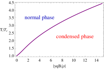
The phase diagram for the lowest Landau level is depicted in figure 9 in the case with fixed charge density . To determine which side of the phase transition line is the condensed phase, we can consider the equation (61). It suggests that the magnetic field decreases the effective mass. So if we increase the magnetic field at a fixed temperature, the normal state will become unstable for sufficiently large magnetic field.
It is clear that the transition temperature increases with the applied magnetic field. In ordinary superconductors an external magnetic field suppresses superconductivity via diamagnetic and Pauli pair breaking effects. However, it has also been proposed that the magnetic field induced superconductivity can also be realized in type-II superconductors [99, 100], in which the Abrikosov flux lattice may enter a quantum limit of the low Landau level dominance with a spin-triplet pairing. And possible experimental evidence for the strong magnetic induced superconductivity can be found, for example, in refs. [101, 102].
Due to the degeneracy in , a linear superposition of the solutions with different is also a solution of the model at . We can take this advantage to construct a class of vortex lattice solutions. As a typical example, the triangular lattice is shown in figure 10. It should be stressed that it is the special combinations which exhibit the vortex lattice structure. Strictly speaking, to obtain the true ground state, one should calculate the free energy of the solutions with different lattice structures from the action to find which configuration minimizes the free energy. It turns out that the linear analysis presented here is not sufficient to determine the most stable solution, thus should include higher order contributions. Furthermore, it is worthwhile to mention that in the AdS soliton background, the external magnetic field triggered phase transition and vortex lattice structure also happen for the vector field p-wave model [103].
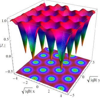
The response of this system to the magnetic field is quite different from the behaviour of ordinary superconductor where the magnetic field makes the transition more difficult. But the result here is quite similar to the case of QCD vacuum instability induced by strong magnetic field to spontaneously developing the -meson condensate [104, 105]. Although so, it was shown that in model (57) the condensate of the vector operator forms a vortex lattice structure in the spatial directions perpendicular to the magnetic field. Of course, the non-minimal coupling term in the action plays a crucial role in both cases. Therefore in some sense, this model is a holographic setup of the study of -meson condensate.
4.2.2 The complete phase diagram
The probe approximation neglecting the back reaction of the matter fields can indeed uncover many key properties. Nevertheless, it still loses some important information, such as the phase structure of the system. In the following paragraphs, we will discuss both the black hole background and soliton background in full back reaction case. Then a complete phase diagram in terms of temperature and chemical potential will be shown. We shall consider a -dimensional bulk theory [106].
We would like to study a dual theory with finite chemical potential or charge density accompanied by a U(1) symmetry, so we turn on in the bulk. We want to allow for states with a non-trivial current , for which we further introduce in the bulk. Because a non-vanishing picks out direction as special, which obviously breaks the rotational symmetry in spatial plane, thus we should introduce an additional function in the component of the metric in order to describe the anisotropy. Therefore, for the matter part, we consider the ansatz
| (62) |
We will consider black hole and soliton backgrounds separately.
(1) AdS black hole with vector hair.
For the black hole background, we adopt the following metric ansatz
| (63) |
The position of horizon is denoted as at which and the conformal boundary is located at . One finds that the component of Maxwell equations implies that the phase of must be constant. Without loss of generality, we can take to be real. Then, the independent equations of motion in terms of above ansatz are deduced as follows
| (64) |
where the prime denotes the derivative with respect to .
When , there exists an exactly analytical black hole solution, namely, AdS Reissner-Nordström black hole which reads
| (65) |
This solution is dual to a conductor phase in the dual field theory. However, the full coupled equations of motion do not admit an analytical solution with non-trivial . Therefore, we have to solve them numerically. We will use shooting method to solve equations (64). In order to find the solutions for all the five functions, i.e., and one must impose suitable boundary conditions both at conformal boundary and at the horizon .
In order to match the asymptotical AdS boundary, the general falloff near the AdS boundary behaves as
| (66) |
where the dots stand for the higher order terms in the expansion of and .212121The has a lower bound as with . In that case, there exists a logarithmic term in the asymptotical expansion of . One has to treat such a term as the source set to be zero to avoid the instability induced by this term [72]. We will always consider the case with . In general, in the above expansion we must impose , which meets the requirement that the condensate appears spontaneously. According to the AdS/CFT dictionary, up to a normalization, the coefficients , , and are regarded as chemical potential, charge density and the component of the vacuum expectation value of the vector operator in the dual field theory, respectively.
We focus on black hole configurations that have a regular event horizon located at and require the regularity conditions at the horizon , which means that all five functions would have finite values at and admit a series expansion in terms of . After substituting such series expansion into equations (64), one finds there are only six independent parameters at the horizon, i.e., and other coefficients can be expressed in terms of those parameters.
Two free parameters and can be fixed by AdS boundary conditions that and . Without loss of generality, the location of can be fixed to be one in our numerical calculation. We are then left with two independent parameters . By choosing as the shooting parameter to match the source free condition, i.e., , we finally have a one-parameter family of solutions labeled by the value of at the horizon. After solving the set of equations, we can read off the condensate , chemical potential and charge density directly from the asymptotical expansion (66).
(2) AdS soliton with vector hair.
To construct homogeneous charged solutions with vector hair in the soliton background, we take the metric as
| (67) |
where vanishes at the tip of the soliton. The asymptotical AdS boundary is located at . Further, in order to obtain a smooth geometry at the tip , should be made with an identification
| (68) |
This gives a dual picture of the boundary theory with a mass gap, which is reminiscent of an insulating phase.
The independent equations of motion are deduced as follows
| (69) |
where the prime denotes the derivative with respect to . Similar to the black hole case, we will solve those coupled equations of motion numerically by use of shooting method. In order to find the solutions for all the six functions one must impose suitable boundary conditions at both conformal boundary and the tip .
The asymptotical expansion for metric fields and matter fields near the boundary is as follows
| (70) |
where the dots stand for the higher order terms of . We choose the source free condition as before. The coefficients , , and are directly related to the chemical potential, charge density and component of the vacuum expectation value of the vector operator in the dual system, respectively.
We impose the regularity conditions at the tip , which means that all functions have finite values and admit a series expansion in terms of as
| (71) |
By plugging the expansion (71) into (69), one can find that there are six independent parameters at the tip . However, there exist four useful scaling symmetries in the equations of motion, which read
| (72) |
| (73) |
| (74) |
and
| (75) |
where in each case is a real positive constant.
By using above four scaling symmetries, we can first set for performing numerics. After solving the coupled differential equations, one should use the first three symmetries again to satisfy the asymptotic conditions , and . We choose as the shooting parameter to match the source free condition, i.e., . Finally, for fixed and , we have a one-parameter family of solutions labeled by . After solving the set of equations, we can read off the condensate , chemical potential and charge density from the corresponding coefficients in (70). It should be noticed that different solutions obtained in this way will have different periods for direction. We should use the last scaling symmetry to set all of the periods equal in order to obtain same boundary geometry. We shall fix to be in this section.
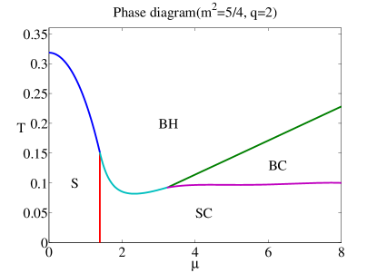
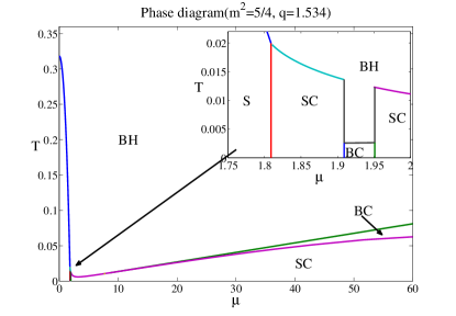

These two kinds of situations have been well studied in ref. [106]. There are four different bulk solutions given by the pure AdS soliton, AdS Reissner-Nordström black hole and their vector hairy counterparts. According to the AdS/CFT dictionary, the hairy solution is dual to a system with a non-zero vacuum expectation value of the charged vector operator which breaks the U(1) symmetry and the spatial rotation symmetry spontaneously. The above four solutions in the bulk correspond to an insulating phase, a conducting phase, a soliton superconducting phase and a black hole superconducting phase, respectively. Since we do not turn on magnetic field, the model is left with two independent parameters, i.e., the mass of the vector field giving the scaling dimension of the dual vector operator and its charge controlling the strength of the back reaction on the background geometry. The phase structure of the model heavily depends on those two parameters. There exist second order, first order and zeroth order222222In the theory of superfluidity and superconductivity, a discontinuity of the free energy was discussed theoretically and an exactly solvable model for such phase transition was given in ref. [107]. The zeroth order transition was also observed in holographic superconductors in refs. [108, 109, 110]. phase transitions as well as the “retrograde condensation” in which the hairy solutions exist only above a critical temperature or below a critical chemical potential with the free energy much larger than the solutions without hair.
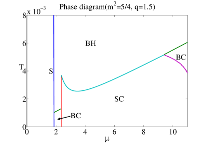
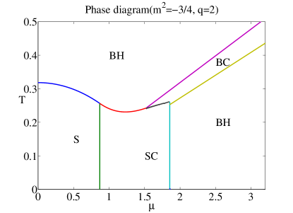
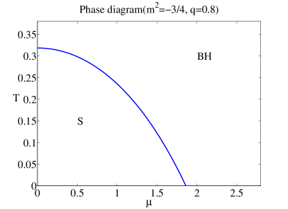
With four kinds of phases at hand, the complete phase diagrams can be constructed in terms of temperature and chemical potential. At each point in - plane, one should find the phase which has the lowest free energy. Since there are many types of phase transitions in both soliton and black hole backgrounds, the - phase diagrams are expected to be much more complicated than the holographic s-wave model [78] and the Yang-Mills p-wave model [84]. Some typical examples are shown in figure 11. We can see from the complete phase diagrams that in some cases, more than one superconducting phase appears in a phase diagram in the model. The phase diagrams for some realistic superconducting materials are usually complicated, and indeed, more than one superconducting phase can occur, for example, see refs. [111, 112, 113]. Definitely, it is of great interest to see whether this model is relevant to those superconducting materials.
4.3 The Helical P-wave model
The gravity solutions above mainly describe spatially homogeneous superconducting states. However, it has long been known that it is possible to have superconducting states that are spatially inhomogeneous. A well known example is the Fulde-Ferrell-Larkin-Ovchinnikov (FFLO) phase, for which a Cooper pair consisting of two fermions with different Fermi momenta condenses leading to an order parameter with non-vanishing total momentum [114, 115]. In this section, we shall introduce a holographic model which can realize p-wave superconducting phase with a helical order. That is to say, the order parameter points in a given direction in a plane which then rotates as one moves along the direction orthogonal to the plane.
We consider a (4+1) dimensional model with a gauge field and a charged two-form [21, 22]
| (76) |
where we have chosen units where the AdS radius is unity, a dagger denotes complex conjugation and the field strengths read
| (77) |
The gauge field is dual to a current in the dual theory and the two-form corresponds to a self-dual rank two tensor operator with scaling dimension . In particular, this charged operator has angular momentum and thus can serve as an order parameter for -wave superconductors. Since what we are interested in is a system at finite temperature and chemical potential with respect to the global U(1) symmetry, we will construct electrically charged asymptotically AdS black holes in gravity side. The normal phase with no condensate is described by the electrically charged Reissner-Nordström AdS black hole, which is spatially homogeneous and isotropic. This model is specified by two parameters and . It was shown in ref. [21] that when this black hole is unstable to developing non-trivial two-form hair that is dual to p-wave superconductors with helical order.
4.3.1 Boundary conditions
The helical black hole solution was constructed in ref. [22] in which the authors adopted the ansatz
| (78) |
where the one-forms are given by
| (79) |
Note that the constant and slices in the above metric are spatially homogeneous of Bianchi type . All eight functions in the ansatz depend on the radial coordinate only and is a constant. After substituting the ansatz into the action (76), one finds that and can be determined by other functions, thus we are left with six independent functions including , , , , and . More precisely, and satisfy first order differential equations and other functions satisfy second order equations.
To solve the coupled equations of motion for above six functions, one needs to specify suitable boundary conditions in the horizon and the conformal boundary . Regularity at the horizon demands that and all of them have analytic expansion in terms of . We then find that the full expansion at the horizon is fixed by six parameters, i.e., and . Near the boundary , one demands asymptotically AdS geometry with the fall-off
| (80) |
which is determined by eight parameters and . One should note that the expansion of is chosen so that the charged operator dual to the two-form has no source, thus can spontaneously acquire an expectation value proportional to which is spatially modulated in the direction with period . and are regarded as the chemical potential and charge density in the dual system respectively. The holographic interpretation of the other UV parameters will be given below. Observe that when the order parameter rotates in the plane as one moves along the direction thus there is a reduced helical symmetry.
There are two scaling symmetries of the coupled equations which can be used to set . To solve the six differential equations, we need to specify ten integration constants. However, we have fourteen parameters in two boundaries minus two for the scaling symmetries. Therefore, we expect to leave with a two parameter family of black hole solutions which can be selected as temperature and wave number .
4.3.2 Thermodynamics
We shall work in grand canonical ensemble with the chemical potential fixed. The thermodynamic potential of the boundary thermal state is identified with temperature times the on-shell bulk action in Euclidean signature. We denote as the density of thermodynamic potential per spatial volume in dual field theory. Then one can obtain the following expression for the free energy density 232323For more details about this result, please see ref. [116].
| (81) |
where the entropy density and is set to be one. From above equation one can immediately obtain the Smarr-type formula
| (82) |
An on-shell variation of the total action for fixed gives us the first law
| (83) |
and hence .
The expectation value of the dual stress-energy tensor is given, after setting , by
| (84) |
Obviously the stress-energy tensor is traceless as a consequence of the underlying conformal symmetry. We further extract the energy density from which we can rewrite and the first law takes the more familiar form . The average hydrostatic pressure is defined as minus the average of the trace of the spatial components. We get , and hence the system satisfies the thermodynamical relation .
4.3.3 Helical p-wave solutions
We focus on the specific case with and 242424The main reason for this choice is to obtain real scaling dimensions. For other values of which can avoid complex scaling dimensions will give similar results [116]. and set . Starting from the AdS Reissner-Nordström black hole solution, as the temperature is lowered, the first instability appears at and . Below , there is a continuum of hairy black hole solutions appearing with different values of .
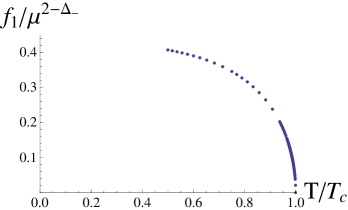
Figure 12 summaries the free energy density as a function of temperature and wave number . One can see that all hairy solutions have smaller free energy than the normal solutions at the same temperature and the transition to the p-wave preferred branch is second order. For a given temperature , there is a one parameter family of solutions specified by , and the most thermodynamically preferred solution is denoted by the red line. One can prove that while the general hairy solutions in figure 12 have , the solutions on the red line do have vanishing [116].
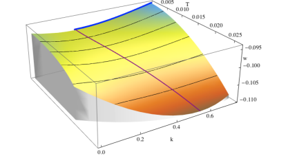
The helical superconducting order can be fixed by the condensate and wave number , which are shown in figure 13 with respect to for the red line in figure 12. Near one can find the critical phenomenon , which is the famous mean field behaviour. As the temperature is lowered, the red line moves smoothly down to sufficiently low temperature at which . In particular, the ground state at is also spatially modulated.
The limit of hairy solutions approach a smooth domain wall solution which interpolates between in the UV and a new IR fixed point with an anisotropic scaling. This fixed point in the IR reads
| (85) |
with and all constants. This fixed point solution is invariant under the anisotropic scaling , , and . All those constants can be determined by the equations of motion.252525Note that one can set by scaling and . As a typical example, choosing and , one can obtain
| (86) |
The domain wall solutions interpolating between the UV fixed point and the IR fixed point can be specified by the wave number [22]. One can see in figure 12 that the limit of the hairy solutions approach these domain wall solutions (the blue line). Similarly, in figure 13, the condensate and wave number for the domain wall denoted by blue dots smoothly connect with the corresponding black hole solution.
To summarize, a holographic p-wave model with helical superconducting order is introduced in this subsection. As the temperature is lowered, a helical superconducting state emerges spontaneously breaking both the abelian symmetry and the three-dimensional spatial Euclidean symmetry down to Bianchi symmetry. These homogeneous, but anisotropic ground states at are holographically described by smooth domain wall solutions, which exhibit zero entropy density and an emergent scaling symmetry in the far IR.
Further nature of the model (76) has been well studied in ref. [116]. For example, some of the p-wave solutions can exhibit the phenomenon of pitch inversion262626As the temperature is lowered, the pitch first increases, becoming divergent (i.e., ) at some particular temperature, then changes sign and finally decreases in magnitude to a value at . and the symmetry of the black hole solutions is enhanced at the pitch inversion temperature. The superconducting phase can also be order. Depending on the mass and charge of the two-form, both the p-wave and the -wave can be thermodynamically favored. The two kinds of orders will compete with each other and there can be first order transition between them.
5 Holographic D-wave Models
It is remarkable to see that rather simple and generic gravity models can capture many features of the phase structure of superconducting systems. Nevertheless, in order to construct more sophisticated and more realistic models one clearly needs to include additional ingredients. The focus of this part is on realising an important missing phase, i.e. d-wave superconductivity (superfluidity). The importance is self-evident since many unconventional superconductors admit either d-wave or mixed symmetry. A natural candidate for modelling the d-wave condensate is to use a charged spin two field in the bulk, instead of a charged scalar field or a vector field. Based on this approach, there are two acceptable holographic models describing the d-wave condensate in the literature.
The authors of ref. [14] first constructed a minimal gravitational model by introducing a symmetric, traceless rank-two tensor field minimally coupled to a U(1) gauge field in the background of an AdS black hole. The d-wave condensate appears below a critical temperature via a second order phase transition, resulting in an isotropic superconducting phase but no hard gap for its optical conductivity. Let us call it CKMWY d-wave model in terms of the initials of the five authors. The other effective holographic d-wave model was proposed soon after the first one with the same matter fields but with much more complex interactions [15]. The phase diagram, optical conductivity, as well as fermionic spectral function were investigated in detail. With a fixed metric, this model has advantages such as being ghost-free and having the right propagating degrees of freedom. This model will be named as BHRY d-wave model for short in what follows.
5.1 The CKMWY d-wave model
To construct a holographic d-wave model, the minimal effective bulk action including gravity, U(1) gauge field and tensor field reads [14]
| (87) |
where is the covariant derivative in the black hole background, is the AdS radius that will be set to unity, and and are the charge and mass squared of , respectively. Working in the probe limit, i.e. with and fixed, the matter part can be treated as perturbations in the 3+1 dimensional AdS black hole background (25).
We would like to realize a d-wave superconductor on the boundary such that a condensate emerges on the plane with translation invariance and the rotational symmetry is broken down to Z(2) with the condensate changing its sign under a rotation on the plane. Therefore, we use an ansatz for and as
| (88) |
with all other field components being turned off and and being real functions. The background geometry is fixed as AdS-Schwarzschild black hole given in (25). Then the final equations of motion read
| (89) |
These two equations are very similar as the case for the Abelian-Higgs model (see equations (27)). Therefore, it is natural to expect to condense spontaneously below a critical temperature. More precisely, we demand the following asymptotic form near the AdS boundary
| (90) |
with . Note that the expansion of is chosen such that the charged operator dual to has no source, thus can acquire an expectation value proportional to spontaneously. According to holographic dictionary, is interpreted as the chemical potential, and as the charge density in the dual theory. The order parameter of the boundary theory can be obtained by reading the asymptotic behaviour of , i.e.
| (91) |
where are the indexes in the boundary coordinates . In what follows, we shall keep the chemical potential fixed and choose to be minus one, which is the setup adopted by ref. [14].
The d-wave condensate as a function of temperature can be obtained numerically, which is shown in figure 14. One can see clearly that below , the tensor field is Higgsed to break the U(1) symmetry spontaneously in the boundary theory. Numerical calculation further ensures that the phase transition characterized by the d-wave condensate is second order with the mean field critical behaviour . The conductivity has also been studied, which uncovered that the AC conductivity is isotropic and below , the DC conductivity becomes infinite but has no hard gap.
5.2 The BHRY d-wave model
The approach of the CKMWY d-wave model just writes down a minimal action for the spin two field without looking in detail at the constraint equations required to get the correct number of propagating degrees of freedom. Soon, the authors of ref. [15] analyzed in more detail the effective action for the spin two field and how the constraint equations could be satisfied. The desired theory for a charged, massive spin two field in a fixed Einstein background takes the following form
| (92) |
where , , and is the Riemann tensor of the background metric. The above theory is ghost-free and describes the correct number of propagating degrees of freedom. The disadvantage is that one has to be restricted to work in a fixed background spacetime that satisfies the Einstein condition . In the context of holographic superconductors, this restriction forces us to work in the probe approximation where the spin two field and gauge field do not influence on the metric. One such a geometry is given by the AdS-Schwarzschild black hole with a planar horizon
| (93) |
The black hole horizon is located at , while the conformal boundary of the spacetime is located at . The temperature of this black hole is
| (94) |
5.2.1 The d-wave condensate
We consider an ansatz where and depend only on the radial coordinate and only the space components of are turned on. According to ref. [15], it is consistent to turn on a single component of and to set other components of the gauge field except for to be zero. Then our ansatz is
| (95) |
with all other components of set to zero, and and real.
With the above ansatz (95), the equations of motion for and are given by
| (96) |
Here the prime denotes the derivative with respect to the radial coordinate . To solve the above coupled equations, one demands that two fields near the boundary should behave as
| (97) |
where . The unitary bound implies that for spin two operators. Therefore, the mass of has a lower bound, i.e. .272727In fact, the previous d-wave model does not consider this aspect. Note that the fall-off of is chosen so that the dual charged operators have no deformation but can acquire expectation value spontaneously. Up to a normalization, the coefficients , and are interpreted as chemical potential, charge density and the expectation value of the component for the spin two operator , respectively. At the horizon, one should require in order to keep being finite at the horizon.
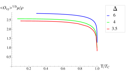
In what follows we will focus on . The resulting boundary value problem can be solved directly, for example, by shooting method. A typical dependence of on the temperature is shown in figure 15. As we lower the temperature, the normal phase becomes unstable to developing tensor hair at a certain critical temperature . This is a typical second order phase transition.
5.2.2 Conductivity
We are interested in the electromagnetic response of the condensed phase. To incorporate this feature, we extract the optical conductivity of this d-wave model by linear response theory. The conductivity tensor can be defined through
| (98) |
where . and are the electric current and electric field, respectively. To compute the conductivity in a holographic framework we turn on a source for the current dual to the gauge field in the bulk. Following the standard approach discussed in previous sections, we perturb the gauge field by . The bulk equations of motion couple linear fluctuations of the gauge field to some spin two components. To obtain a consistent set of equations, one should also turn on time dependent fluctuations of the complexified fields , , and . The linearized equations of motion for the component of these fluctuations are [15]
| (99a) | ||||
| (99b) | ||||
| (99c) | ||||
The equations for and can be obtained by complex conjugation and an additional transformation to from the last two equations. The functions and can be eliminated from the first two equations by virtue of (99), leaving three coupled differential equations for , and . Since the fluctuation decouples from above set of fluctuations, we can conclude that the Hall conductivity is vanishing.
The conductivity is related to the retarded Green’s function for the charge current. To calculate the retarded function, one should impose causal boundary conditions on the equations of motion. As a consequence, the near-horizon modes of the gauge field and spin two field are falling into the horizon, i.e., , and have the behaviour as
| (100) |
Near the boundary , the asymptotical behaviour for the perturbation fields , and is given by
| (101) | |||||
with . Here and are identified as the source terms, while and are the normalizable fluctuations. Since the presence of source terms and will also source the U(1) current, one should look for solutions where the source in the series expansion of and should vanish. Finally, one can obtain the conductivity in the direction as
| (102) |
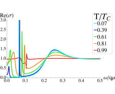
In order to obtain the conductivity in the direction, we look at the effect of a rotation of the condensate in equations (99). This rotation operation flips the sign of , which is equivalent to flipping the sign of by viewing of the equations of motion. Changing the sign of is equivalent to flipping the sign of both the electric field (the term) and the current (the term), thus conductivity will be unaffected under such a change of sign. This implies that the conductivity is proportional to the identity matrix. In fact, the isotropy of conductivity is a consequence of the symmetries that has in the d-wave case. An isotropic conductivity for a d-wave superconductor can be also produced in an explicit microscopic model [117].
The numerical results for the conductivity are shown in figure 16 for a d-wave condensate of conformal dimension . As the temperature is lowered one can observe a spike in the conductivity, which is a signal of a bound state. This spike is localized at smaller values of as the temperature is lowered. A second spike in the conductivity appears to disappear as the temperature is decreased. One can also see that does not vanish even for arbitrary small frequency , so there is no hard gap in the dual boundary superconducting phase.
The fermionic spectral function in this holographic superconductor with a d-wave condensate has been well studied in ref. [118]. It was showed that, with a suitable bulk Majorana coupling, the Fermi surface is anisotropically gapped. At low temperatures the gap shrinks to four nodal points, while at high temperatures the Fermi surface is partially gapped generating four Fermi arcs. The condensate for the BHRY model was investigated in ref. [119], in which the existence of fermi arcs is confirmed and a non-vanishing Hall conductivity is obtained in the absence of a magnetic field.
Although both d-wave models we reviewed above can be used to study the properties of a superconducting phase transition with a d-wave order parameter in a dual strongly interacting field theory, the construction is not ideal. For example, the BHRY d-wave model can only work in the probe limit. However, it is well known that including the back reaction of matter fields would lead to a much richer phase structure. It will be desirable to study a consistent holographic d-wave model with back reaction. To write down an action for a charged spin two field propagating in a curved spacetime is challenging, because it usually suffers from non-hyperbolic and non-causal behaviour of the spin two field. Apart from those two effective models, the authors of ref. [120] discussed top-down models for holographic d-wave superconductors in which the order parameter is a charged spin two field in the bulk.
6 Competition and Coexistence of Superconducting Order Parameters
The holographic models of s-wave, p-wave and d-wave superconductors, which have scalar, vector and spin-2 order parameters respectively, have been discussed in the previous sections. These models were based on a specific setup where the dynamics in the bulk involves only a single order parameter. It is desirable to generalize the single order parameter case to multi order parameters case because the real high superconducting systems indeed involve various orders, such as magnetic ordering and superconductivity, see figure 17 and, e.g., refs. [122, 123]. The holographic correspondence provides us a convenient way to investigate the interaction for these orders by simply introducing dual fields in the bulk as well as appropriate couplings among them. Following this strategy, several works on the competition of multi order parameters in the holographic superconductor models have already been made [124, 125, 126, 127, 128, 129, 130, 131, 132, 133, 134]. In the following, we will review the competition between two s-wave orders [124], the competition between s-wave order and p-wave order [125, 126] and the competition between s-wave order and d-wave order [127] one by one. The first case concerns the competition between two orders with the same symmetry and the last two cases are to study the competition of orders with different symmetry. The phase diagrams are also drawn for the corresponding models.
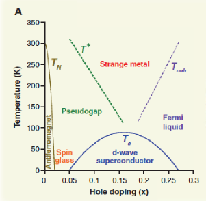
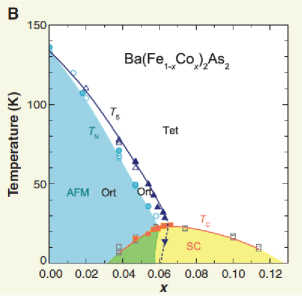
6.1 Competition and coexistence of two s-wave orders
Historically, Ginzburg-Landau theory has proved to be an extraordinarily valuable phenomenological tool in understanding single-component superconductors. Its generalization to the two-component Ginzburg-Landau model (TCGL) was constructed, and its applicability to the two-band systems studied in refs. [135, 136, 137]. Upon switching on the interband coupling between the two components, this model can describe the phenomenon of the two gaps in materials such as MgB2 () [138, 139] and iron pnictides () [140, 141, 142]. Applying the multi-band Ginzburg-Landau theories to the gravity side, the holographic multi-band superconductor model can be realized involving some competing scalar fields coupled to a single gauge field. Such system exhibits rich phase structure. Next, we will describe the holographic model concretely and show results explicitly.
6.1.1 The holographic model
Let us start a holographic superconductor model with scalar hairs in dimensional anti-de Sitter spacetime. The action reads [124]
| (103) |
where and () are the charge and mass of the scalar field , respectively. The term denotes the possible interaction among bulk matter fields. Here one can perform a rescaling of the type to set the charge of the scalar field to unity. We are interested in the dynamics and mutual interaction among different orders. Here we limit ourselves to the case with . The concrete model we will study is described by the following action
| (104) |
where we have defined and . The parameter controls the strength of the back reaction and is the effective charge of or the ratio of two scalar charges.
The hairy black hole solution is assumed to take the following metric form
| (105) |
together with homogeneous matter fields
| (106) |
The horizon is determined by and the temperature of the black hole is given by
| (107) |
One can use the U(1) gauge symmetry to set to be real. After using the component of Maxwell’s equations we can also safely choose to be real. We will work in the unites where . Then, the independent equations of motion in terms of the above ansatz are deduced as follows
| (108) |
where a prime denotes the derivative with respect to .
The gravity background describing the normal phase is just the AdS Reissner-Nordström black hole with a planar horizon
| (109) |
where is the black hole horizon and is the chemical potential of the black hole.
6.1.2 Phase transition
The two band model is controlled by four model parameters, i.e., , , , and . Here we will choose and . One may expect that the model admits three different superconducting phases. The first superconducting phase corresponds to the case with and (Phase-I). The second superconducting phase corresponds to the case with and (Phase-II). The third superconducting phase admits the region where both scalars condense simultaneously.
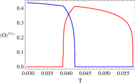
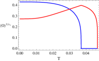
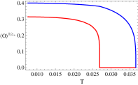
The numerical results are shown in figure 18. The model admits three kinds of the coexisting phase. The first kind is shown in the left panel of figure 18. As we lower temperature, the scalar first condenses at where the superconducting phase transition happens; when we continue lowering temperature to a certain value, say , the scalar begins to condense, while the condensate of decreases, resulting in the phase with both orders; if one further lowers temperature, the first condensate quickly goes to zero at a temperature ; when temperature is lower than , there exists only the condensate of . This superconducting phase is denoted by Phase-C and it is the case uncovered in the probe limit in ref. [129]. The second kind of the coexisting phase is presented in the middle plot. It is different from the first one in that the coexisting phase survives even down to a low temperature. We denote this case by phase-A. Depending on the back reaction, the inverse of phase-A is also true: the condensate of emerges following the condensate of , and then both orders are always present. This case is labeled as Phase-B drawn in the right plot.
To determine whether those above three coexistence phases are thermodynamically favored in their own parameter spaces, one should calculate the free energy of the system for each phase. Working in grand canonical ensemble, the chemical potential is fixed. In gauge/gravity duality the grand potential of the boundary thermal state is identified with temperature times the on-shell bulk action with Euclidean signature. The Euclidean action must include the Gibbons-Hawking boundary term for a well-defined Dirichlet variational principle and further a surface counter term for removing divergence. Note that we are considering a stationary problem, the Euclidean action is related to the Minkowski one by a minus sign as
| (110) |
where is the determinant of the induced metric on the boundary , and is the trace of the extrinsic curvature. By using of the equations of motion (108) and the asymptotical expansion of matter and metric functions near the AdS boundary, the grand potential can be expressed as
| (111) |
where and the constant is from the asymptotical expansion of . For the normal phase given in (109), one has .
The free energy corresponding to phase-A(C) is drawn in figure 19. From each plot, phase-A(C) does have the lowest free energy, indicating that once phase-A(C) appears, it is thermodynamically favored. But for phase-C, there is only a narrow window admitting the two orders to coexist. Comparing phase-B with phase-A, the only difference is that condenses before . From figure 19, one can also see there exist two transition points in both cases. One is the critical superconducting phase transition and the other within the superconducting phase, which indicates the fact that our system is multi-band. In order to see this clearly, one can define the total condensate as , and draw as a function of temperature in figure 20. As one lowers temperature, emerges at the critical superconducting phase transition point, then at a certain temperature inside the superconducting phase it has a sudden increase, where the condensate of the other appears. Such a behaviour is very reminiscent of the one in the real multi-band superconductor.
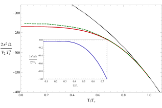
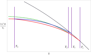
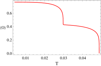
6.1.3 Conductivity
In order to ensure the system is indeed in a superconducting state, one should calculate the conductivity . Since now the back reaction is included, one has to consider the fluctuations of and . Assuming both perturbations have a time dependence of the form , the final equation of motion to calculate the conductivity can be obtained as
| (112) |
Since the conductivity is related to the retarded two-point function of the U(1) current, i.e, , one imposes the ingoing boundary condition near the horizon
| (113) |
with being constants. The gauge field near the boundary falls off as
| (114) |
According to the AdS/CFT dictionary, the retarded Green function can be read as , from which one can obtain the conductivity
| (115) |
The optical conductivity as a function of frequency in the region with two order parameters is presented in figure 21. One can see clearly that the optical conductivity in two band model behaves qualitatively similar to the model with only one scalar order discussed in figure 2. In addition, from the Kramers-Kronig relations, one can conclude that the real part of the conductivity has a Dirac delta function at since the imaginary part has a pole, i.e., Im.
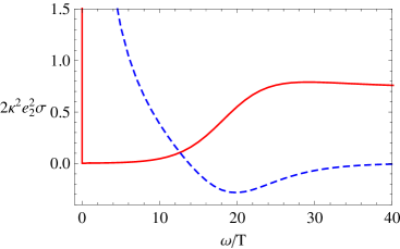
6.1.4 Phase diagram
Constructing the parameter space is helpful to learn in which region the superconducting orders can coexist. One can complete this task by just turning the problem as an eigenvalue problem. Focus on the concrete model discussed in this paper, i.e., and , a good starting point is to find the critical valve of the ratio such that is a critical temperature at which begins to vanish or emerge. At such a temperature, is very small and can be treated as a perturbation on the background where only condenses
| (116) |
where are functions describing the hairy AdS black hole with only non-vanishing. Imposing the appropriate boundary conditions, this equation can be considered as an eigenvalue problem with positive eigenvalue . The full phase diagram for the five superconducting phases is shown in figure 22.
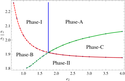
From figure 22, one has as many as five superconducting phases in the model apart from the normal phase. Depending on the model parameters and , each phase can be most thermodynamically stable in some region of parameter space. As one increases the strength of the back reaction, the region for Phase-C with the coexisting behaviour of two order parameters only in a narrow window is gradually forced to shrink and finally vanishes at , while the regions for Phase-A and Phase-B where both order parameters always present enlarge. In this sense, one can conclude that the gravity which provides an equivalent attractive interaction between the holographic order parameters tends to make the coexistence of two orders much more easy rather than more difficult.
In this subsection 6.1, a holographic superconductor model with more than one order parameter in four dimensions has been studied, where each complex scalar field in the bulk is minimally coupled to a same U(1) gauge field. This can be interpreted as a holographic multi-band superconductor model. Concretely, we have discussed the two-band case with mass squares and for two bulk scalar fields and , respectively. Depending on the strength of the back reaction and the relative charge ratio of the two scalar fields, the model admits as many as five different superconducting phases. Three of them, denoted by Phase-A, Phase-B and Phase-C, exhibit the coexistence region of two order parameters. More specifically, for Phase-C, as one lowers the temperature, the second scalar condenses following will completely suppress the condensate of the first order, i.e., will go to zero finally. The condensate behaviours in Phase-A and Phase-B are similar. One of the two orders condenses first, and once the other begins to condense, both always coexist. However, this model is limited to the competition of the order parameters with the same asymmetry. Therefore it is quite interesting to study the holographic models with superconducting order parameters with different spins. This will be done in the following subsections.
6.2 Competition between s-wave and p-wave orders
In this subsection, we will study two holographic superconductor models with both s-wave and p-wave condensed. One is proposed in ref. [125], where the authors built a holographic superconductor model with a scalar triplet charged under an SU(2) gauge field in the bulk. The other holographic s+p model in ref. [126] consists of a scalar doublet charged under an U(2) gauge field living in a planar Schwarzschild black hole geometry. The discussions for both models are limited to the probe limit case.
6.2.1 The holographic s+p superconductor with a scalar triplet charged under an SU(2) gauge field
To realize the s-wave and p-wave superconductivity in one model, we first consider a real scalar triplet charged in an SU(2) gauge field in the gravity side. The full action is [125]
| (117) |
where is an SU(2) charged scalar triplet in the vector representation of the SU(2) gauge group, and
| (118) |
is the gauge field strength which is the same as (43) and reads
| (119) |
is the Yang-Mills coupling constant as well as the SU(2) charge of . One can redefine the fields and to get the standard expression where the coupling appears in the derivative operator . Here we limit ourselves to the case of probe limit. This limit can be realized consistently by taking the limit .
In the probe limit, we consider the dimensional AdS black brane as the background with metric
| (120) |
s are the coordinates of a dimensional Euclidean space. The function is
| (121) |
with the horizon radius. Here the AdS radius has been set to be unity. The temperature of the black brane is related to as
| (122) |
This is just the temperature of dual field theory in the AdS boundary.
Let us consider the following ansatz for the matter fields
| (123) |
with all other field components being turned off. In this ansatz, we take as the electromagnetic U(1) field. With this ansatz, the equations of motion of matter fields in the AdS black brane background read
| (124) | |||||
One can see and are not coupled in their equations of motion, but they are both coupled to the same U(1) electromagnetic field. In this model, thus one can easily realize the s-wave and p-wave superconductivity consistently.
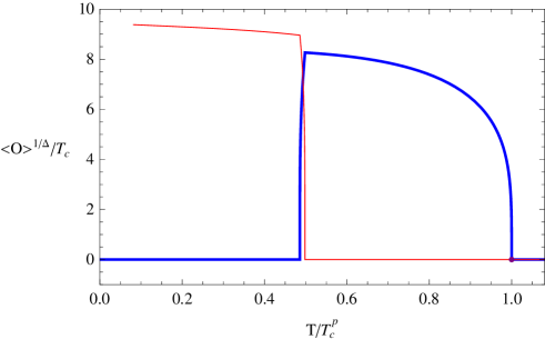
We take the case with as an example. The condensate behaviour for the coexisting phase is drawn in the left plot of figure 23. We can see that the coexisting phase starts from the p-wave phase and ends with the pure s-wave condensate phase. Based on the calculation of free energy shown in figure 24, we confirm that the s+p coexisting phase indeed has the lowest free energy and is thus thermodynamically favored in the temperature region. Thus the potential first order phase transition from the pure p-wave phase to the pure s-wave phase is replaced by the phase transitions from the p-wave phase to the s-wave phase through an s+p coexisting phase. And all the three phase transitions are continuous ones, and are of characteristic of second order phase transition within the numerical accuracy.
From figure 24, we see that the Gibbs free energy curves of the s-wave and p-wave phases have an intersection when . The s+p coexisting phase just exists in this interval. By computing the values of and and getting the relations and in the region , a phase diagram of the holographic model on the – plane can be shown in figure 25. We can see from the figure that the system contains four kinds of phases known as the normal phase, the s-wave phase, the p-wave phase and the s+p coexisting phase. The s+p coexisting phase is favored in the area between the blue line and the red line. The region for the s+p coexisting phase is very narrow in the phase diagram. This is similar to the situation of the coexisting phase with two s-wave orders in the probe limit studied in ref. [129]. However, for the latter, the region with the coexisting phase is enlarged with the full back reaction [124]. This would be due to the additional interaction between the two scalar fields in the bulk through gravity and this interaction reduces the repellency between the two condensates.
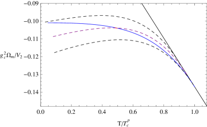
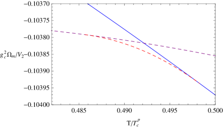
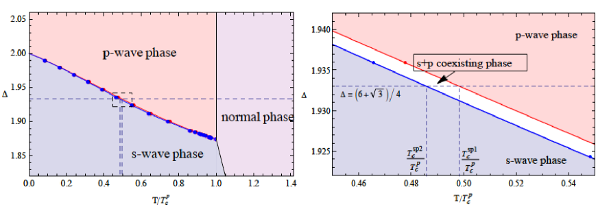
Very recently, the back reaction effect was included in this model [143], which showed a rich phase structure and various condensate behaviours such as the “n-type” and “u-type” ones. The phase transitions to the p-wave phase or s+p coexisting phase become first order in strongly back reacted cases. The phase diagrams similar as figure 25 in different strength of back reaction were constructed, indicting that the region for the s+p coexisting phase is enlarged with a small or medium back reaction parameter, while is reduced in the strongly back reacted case.
6.2.2 The holographic s+p superconductor with a scalar doublet charged under a U(2) gauge field
In this sector, we consider a holographic s+p model consisting of a scalar doublet charged under a U(2) gauge field living in a -dimensional Schwarzschild-AdS black brane geometry. The action for the matter sector reads [126]
| (125) |
with
| (126) | |||
The system lives in the Schwarzschild-AdS background (120). Considering the following consistent ansatz for the fields
| (127) |
with all functions being real-valued, the resulting equations of motion read
| (128) |
In what follows we choose the scalar to have and thus the corresponding dual operator has mass dimension 2.
The UV asymptotic behaviour of the fields, corresponding to the solution of equations (128) in the limit , is given by
| (129) |
where in the dual field theory side, and are respectively the chemical potential and charge density corresponding to the overall generated by , whereas and are the chemical potential and charge density corresponding to the generated by . is the source of a scalar operator of dimension 2, while is its expectation value. Finally and are the source and vacuum expectation value of the current operator . Notice that in a background where condenses the is spontaneously broken, and moreover spatial rotational symmetry is spontaneously broken too.
We are looking for solutions of the equations (128) where , , or both acquire non-trivial profiles. First we will switch on a chemical potential along the overall U(1), while requiring that the other chemical potential remains null. Therefore the UV boundary conditions are
| (130) |
In the IR regularity requires to vanish at the black hole horizon. So far, the holographic multi-component superfluid model has been realized.
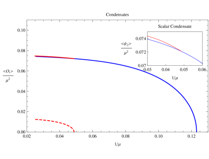
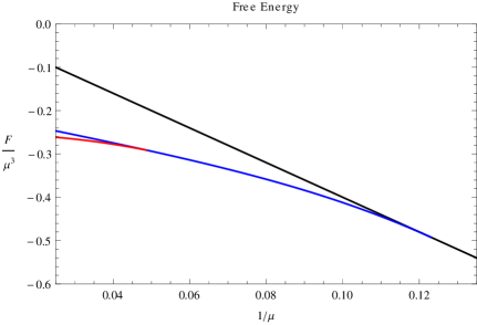
In the left plot of figure 26 the condensates and are plotted as a function of the chemical potential. Notice that the solution where both condensates coexist extends down to as low as where the decoupling limit is trustable. And the free energy for the different solutions is shown in the right plot of figure 26. At small chemical potential only the normal phase solution exists. At there is a second order phase transition to the s-wave solution. If one keeps increasing , at there is a second order phase transition from the s-wave phase to the s+p-wave phase. The system stays in the s+p-wave phase for .
Next, we relax the condition and study the phase diagram of the system as a function of and . Notice that turning on a second chemical potential means to explicitly break . The system can now be interpreted as a holographic dual to an unbalanced mixture. The UV boundary conditions now read
| (131) |
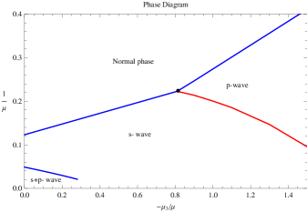
In this case, by computing the free energy of the different solutions, the phase diagram of the system as a function of and is plotted in figure 27. For small values of , the solution where both condensates coexisting extends down to as lower as where we can trust the decoupling limit. As gets larger, the transition to the s+p-wave phase happens at a higher value of . For is large enough, the p-wave phase is preferred at intermediate values of . Therefore, as is increased above a critical value the system goes from the normal to the p-wave phase through a second order phase transition. If is increased even further a first order phase transition takes the system from the p-wave to the s-wave phase. The tricritical point where the normal, s-wave and p-wave phases meet happens at and , the p-wave solution is never energetically preferred for .
In summary, in this subsection we have reviewed the competition between s-wave and p-wave order through two holographic superconductor models. The first model is realized the s+p superconductor with a scalar triplet charged under an SU(2) gauge field and the other is constructed with a scalar doublet charged under a U(2) gauge field. The s+p coexisting phase exists in both models. In the first model, the s+p coexisting phase is narrow and one condensation tends to kill the other. This competing behaviour is similar to the case shown in the condensed matter system [144]. However, in the second case, the condensates feed on different charge densities and the coexisting phase survives down to a low temperature. Therefore, it should be noted that the competing scenario is model dependent. In next subsection, we will study the competition between the scalar field and the tensor field, i.e., the competition between the s-wave and d-wave orders.
6.3 Competition between s-wave order and d-wave order
In section 5, we have mentioned two acceptable holographic models describing the d-wave condensation. The CKMWY d-wave model is reviewed in subsection 5.1 and the BHRY d-wave model in subsection 5.2. In order to realize the condensation of s-wave order and d-wave order in one holographic model, one can simply combine the Abelian-Higgs model with a d-wave model. Thus, one could have two holographic models with s-wave order and d-wave order. Here we will discuss the competition between s-wave order and d-wave order for both d-wave models in the probe limit where one neglects the back reaction of matter fields to the background geometry [127]. The phase structures are given and the behaviours of the thermodynamic quantities for the s+d coexisting phase are also studied. The coexisting phase does appear in both models and is thermodynamically favored.
6.3.1 The s-wave + BHRY d-wave model
To study the competition between s-wave and d-wave orders, let us first start with the holographic model by combining the Abelian-Higgs s-wave model and BHRY d-wave model. The holographic model with a scalar field , a symmetric tensor field and a U(1) gauge field is described by the following action [127]: 282828Ref. [128] also discussed the following model, but with a coupling between the scalar field and the tensor field, and studied the phase structure in terms of the coupling parameter and temperature with fixed charges of two orders. In the folloowing discussion, there is no direct interaction between scalar and tensor fields and the model parameter is the ratio of two fields. Note that in paper [128], when the coupling , there also exists a coexisting phase under the model parameters and . Both results are consistent with each other in that case.
| (132) |
where and , , and is the Riemann tensor of the background metric. is the scalar order and is the tensor order. The parameters and are the charges of the scalar and the tensor fields, respectively. One can perform a rescaling to set the charge of the scalar to be unity. Then the phase structure of this theory is determined by the ratio by fixing the mass square of the scalar field and the mass square of the tensor field . We shall set without loss of generality in the following discussion.
Working in the probe limit, we choose the background metric to be the 3+1 dimensional AdS-Schwarzschild black hole with planar horizon (120). And we consider the following ansatz
| (133) |
with , and all real functions.
With the above ansatz (133), the equations of motion for , and are given by
| (134) |
Here the prime denotes the derivative with respect to . With this model at hand, we can study the competition mechanism between the s-wave order and d-wave order. It is easy to see that equations (134) have a symmetry
| (135) |
Under this symmetry transformation, the role of s-wave and d-wave would interchange each other. Without loss of generality, here we focus on the case .
Before solving the set of coupled equations (134) numerically, we make a briefly qualitative analysis on the possible phases for such a model. Following ref. [129], we rephrase the equations for the s-wave and d-wave as a potential problem. The evolution equations for s-wave and d-wave in equations (134) can be rewritten as follows
| (136) |
where with and and . Now in terms of the new variable , the equations of motion for s-wave and d-wave are rephrased as a potential problem on a semi infinite line, i.e., . Our qualitative discussion is based upon the lemma proven in ref. [129]. For the case , no matter which gauge field configuration we choose, we always have . Therefore the phase structure of the system is the same as that of s-wave holographic superconductor with a single scalar. While, for the case , one may expect that the d-wave field with large charge will always dominate. However, the potential diverges like near the boundary when we lower the temperature. Therefore, lowering the temperature possibly makes the mass dependent potential more important and hence the s-wave tends to dominate. We will confirm this with the following numerical calculation.
Here we set the mass square and and we take as a typical example. Our numerical results confirm that the model does admit the coexistence region of two orders with different symmetry, which is drawn in figure 28. We find that the s+d coexisting phase starts from the d-wave phase and ends with the pure s-wave condensate phase. The calculation of the free energy confirms that the coexisting s+d phase is thermodynamically favored as shown in figure 29.
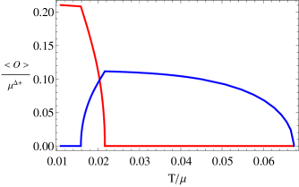
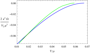
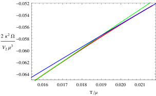
Based on the above discussions, it can be seen clearly that there exist three particular points at which the derivative of the charge density with respect to temperature is discontinuous, indicating a second order phase transition. The one with the highest temperature is the critical point for the superconducting phase transition, while the remaining two points are inside the superconducting phase, indicating the appearance and disappearance of coexisting phase. We can also see the signal of phase transition from the behaviour of the total charge density as a function of temperature and the ratio versus temperature shown in figure 30, where is the superconducting charge density and is the normal charge density carried by the black hole.
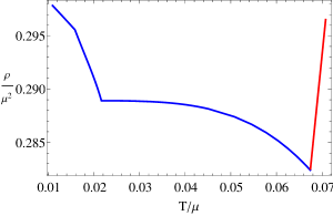
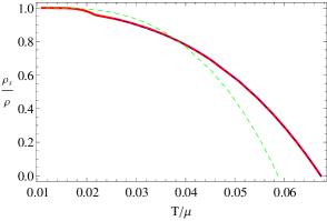
In order to ensure the system is indeed in a superconducting state, we calculate the optical conductivity , which corresponds to the red line shown in figure 31. We see that much more interesting phenomena happen in the low frequency region. Unlike the s-wave case which only has a bump at in figure 31, for pure d-wave condensate, apart from a much more obvious bump at , Re() has an additional spike at a lower frequency. This spike may indicate the existence of a bound state [15]. One can see clearly that such peak becomes much more sharper in the s+d coexisting state, thus the bound state is enhanced due to the additional condensate of s-wave order.
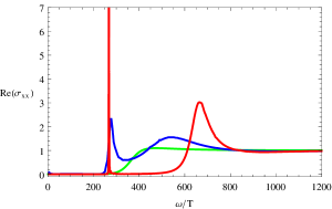
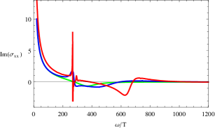
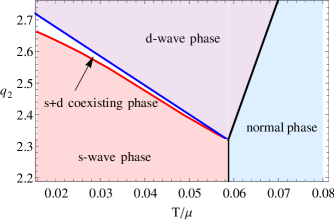
To be complete, we give the phase diagram with and shown in figure 32, which can tell us in which region the coexisting phase appears. From figure 32, we see that the coexisting phase exists only in a narrow region in the phase diagram. We denote the critical temperature for a single s-wave or d-wave starting to condense as and . If we set the charges of the s-wave and d-wave fields to unity, then and . We see that
-
•
In the regime , the s-wave dominates the system and there is no condensation of the d-wave order.
-
•
As increases beyond , the s+d phase appears, which emerges from the d-wave phase and ends with a pure s-wave.
-
•
If we continue increasing to the case , the s-wave order never condenses and the resulting phase diagram is the same as that of model with only d-wave order.
Finally, we try to give a qualitative explanation on the mechanism through which the condensation of one order affects the dynamics of the other order. Note that here the back reaction is not taken into account. Thus the two fields interact only through their effect on the gauge field once one or both has (have) condensed. Through looking at the gauge field we may give some insight into the competing mechanics between two orders.
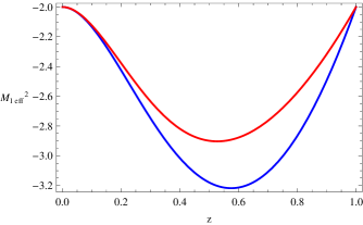
-
•
First, after the d-wave order condenses, if one keeps lowering the temperature and reaches the critical temperature at which the pure s-wave would condense, this condensation does not happen. This is due to the fact that the condensation of the d-wave increases the effective mass of the s-wave, thus prevents the instability of the s-wave to happen, which can be seen from figure 33. This reflects the competition between s-wave and d-wave.
-
•
However, further decreasing the temperature, the condensation of s-wave does happen. This is due to the fact that the effective mass of the s-wave is lowered and ultimately even if the condensation of the d-wave depleted the gauge potential, the background with only d-wave order becomes unstable.
-
•
Finally, the condensate of the s-wave order kills the first one. This should be due to the effective mass square of the s-wave being lower.
It should be noted that this phenomenon is model dependent. This narrow coexistence region of two superconducting orders and the fact that one condensate can eventually kill the other also happen for two s-wave orders in ref. [129] and the s+p case in ref. [125]. The competition diagram is similar to the competition between the conventional s-wave and the triplet Balian-Werthamer or the B-phase pairings in the doped three dimensional narrow gap semiconductors, such as and in the condensed matter system [144]. Although in ref. [144] the competition is apparently between a s-wave order and a p-wave order, d-wave and p-wave are similar in some circumstances, for example, their excitations of the normal component can be probed using low frequency photons.
6.3.2 The s-wave + CKMWY d-wave model
With the same strategy, in this subsection we study the competition between s-wave order and d-wave order in the model combining the Abelian-Higgs s-wave model [11] with the CKMWY d-wave model [14]. The full action including a U(1) gauge field , a complex scalar field and a symmetric, traceless tensor field takes the following form [127]
| (137) |
with
| (138) |
Here and . In the probe limit, matter fields can be treated as perturbations in the 3+1 dimensional AdS black hole background (120). Let us consider the following ansatz
| (139) |
with all other field components being turned off and , and being real functions. Then the explicit equations of motion read
| (140) |
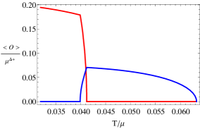
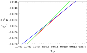
The numerical results are shown in figure 34 for the case with , , and . As seen, a new phase with both s-wave order and d-wave order coexistence can appear near and this s+d coexisting phase has the lowest free energy and is thus thermodynamically preferred to the s-wave phase and d-wave phase. In more detail, as we lower the temperature of the system, it first undergoes a phase transition from the normal phase to the pure d-wave phase at . Then at , a new phase transition occurs, and the system goes into an s+d coexisting phase. Finally the system undergoes the third phase transition from the s+d coexisting phase to a pure s-wave phase at . Note that all the three phase transitions are second order.
The feature of the phase transitions can also be seen clearly from the charge density as the function of temperature in figure 35. One can see that the charge density with respect to temperature is continuous, but its derivative is discontinuous at three special points, indicating three second order phase transitions. These features are the same as those for the model in the previous subsection. But there is a little difference in the behaviour of the total charge density for the d-wave phase. In the s-wave + BHRY d-wave model, the total charge density changes monotonously with the temperature, while it behaves non-monotonous in the present case.
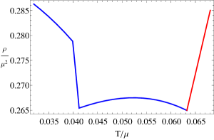
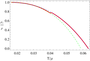
The information of the phase transitions can also be revealed via the behaviour of the ratio with respect to the temperature. From figure 36, one can see that the ratio also has a small kink in the region of the coexisting phase. Comparing figure 30 with figure 36, we see that in the former case, the green dashed curve for the pure s-wave phase intersects with the blue dashed curve for the pure d-wave phase. In contrast, the green dashed curve in figure 36 is always lower than the blue dashed curve. Therefore, as one lowers the temperature, the ratio in the s+d coexisting phase increases for the former (132), while it decreases for the latter (137). The authors of ref. [125] investigated an s+p coexisting phase and found the decrease of the ratio in the coexisting phase, similar to figure 36. They suggested that it might be an experimental signal of the phase transition from a single condensate phase to a coexisting phase. Nevertheless, the results here uncover that the ratio versus temperature is model dependent.
The phase diagram for the model (137) with and in the plane is shown in figure 37. As the s-wave + BHRY d-wave model, the system also contains four kinds of phases known as the normal phase, s-wave phase, d-wave phase and s+d coexisting phase. The normal phase dominates in the high temperature region, the s-wave phase dominates in the lower temperature region with small below the red curve, and the d-wave phase dominates in the higher temperature zone with large above the blue curve. The s+d coexisting phase is favoured in the area between the red and blue curves. The region for the s+d coexisting phase is very narrow in the phase diagram, which indicates that the s-wave and d-wave phases generally repel each other, but they can coexist in a very small range of temperature.
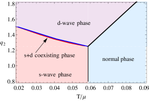
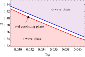
Comparing the two holographic setups, i.e., the model (132) and the model (137), one can see some common features as follows.
- •
-
•
All phase transitions are second order in these two holographic models.
- •
There exist also some differences in the two models. For suitable model parameters in the first model, as the temperature is lowered, the s-wave order condenses inside the d-wave order resulting in the coexisting phase with both orders. However, when the scalar order condenses the first one starts to disappear, and finally only the s-wave condensate is left for sufficiently low temperatures. If one changes the model parameter , the inverse is also true: the condensate of d-wave order emerges following the condensate of s-wave order, and then the d-wave condensate finally kills the s-wave order. Those two kinds of coexisting phase are one to one correspondence. In contrast, in the second model, one sees only the first kind of the coexisting phase. What’s more, for the first model, the ratio increases in the s+d coexisting phase as the temperature is lowered, while it decreases in the second case. This gives an obvious evidence that the ratio versus temperature is model dependent.
7 Coexistence and Competition of Magnetism and Superconductivity
The novel paired mechanism makes p-wave superconductor have many features which are different from the traditional knowledge coming from s-wave superconductor both in theories and experiments. In the usual picture, superconductivity and magnetism are incompatible with each other. Especially, ferromagnetic phase, a spontaneously magnetized phase which has nonzero magnetic moment without external magnetic field and appears when the temperature is lower than a critical one called “Curie temperature”, can not coexist with superconductivity at a sample.292929However, under special conditions superconductivity may coexist with antiferromagnetic order, where neighboring electron spins arrange in an antiparallel configuration. Since antiferromagnets don’t have net magnetism, we won’t involve them here. This is rooted in the microscopic theory of superconductivity from BCS theory. However, this understanding is broken by p-wave superconductor. The discovery of the superconducting ferromagnet303030We will use “superconducting ferromagnet” to denote the materials whose Curie temperature is higher than superconducting transition temperature and “ferromagnetic superconductor” to denote the opposite case. materials, such as UGe2 [145], URhGe [146], UCoGe [147] and ZrZn2 [148], came as a big surprise. In this material, superconductivity is realized well below the Curie temperature, without expelling the ferromagnetic order.
The nature of superconducting state in ferromagnetic materials is currently under debate. For a review of phenomenological theory of ferromagnetic unconventional superconductors with spin-triplet Cooper pairing of electrons, one can see refs. [149, 150, 151]. However, the microscopic theory about the coexistence of magnetism and superconductivity in strongly interacting heavy electrons is either too complex or insufficiently developed to describe the complicated behaviour. So it is still a fascinating thing to find a suitable theory to describe the coexistence and competition of the ferromagnetism and superconductivity in strong correlated system.
Holographic frame to discuss the coexistence and competition between spontaneously magnetic order phase and superconductivity initiated in refs. [132, 152]. Because of lacking an individual model to describe spontaneously magnetization and the time reversal symmetry broken, these models cannot give complete features of this topic. A very new idea proposed in ref. [153] tries to give an independent model describing spontaneously magnetization in holographic frame, which opens a new direction. We will introduce the main results in this framework. For more details, one can refer to refs. [153, 154, 155].
7.1 The holographic model for ferromagnetism/paramagnetism phase transition
Before going on the topic of coexistence of ferromagnetism and superconductivity, let’s first review how to build a holographic ferromagnetism which is independent on superconductivity in ref. [153]. This model is realized by adding a real antisymmetric field into Einstein-Maxwell theory in a (3+1) dimensional AdS spacetime,
| (141) |
where
| (142) |
Here and is the Newtonian gravitational constant, and are two constants, is the mass of the real tensor field , is the gauge potential of U(1) gauge field. The antisymmetric tensor field is the effective polarization tensor of the U(1) gauge field strength with the self-interaction which should be expanded as the even power of . The probe limit corresponds to . Under this limit, the equation for polarization field decouples from the gauge field and gravity field,
| (143) |
with the dyonic Reissner-Nordström (RN) background [156],
| (144) | |||||
Here the horizon radius has been scaled to be unitary. If we only care about the magnetic part of polarization field, then a self-consistent ansatz for polarization field is . Taking this ansatz into equation (143), we have
| (145) |
where a prime denotes the derivative with respect to . It is interesting to see that these two equations decouple from each other in this case, which makes it to be possible that we can neglect the dynamic of if we only care about the dynamic of magnetism. At the horizon, we need to impose a regular boundary condition. Near AdS boundary, the linearized equations have following asymptotic solutions for ,
| (146) |
with . In order to make the theory self-consistent and spontaneous condensation appear, we need following restriction on parameters,
| (147) |
According to the action (141) one can derive the magnetic moment from polarization field, which reads
| (148) |
Here we have set the constant in this expression for convenience. This integration converges only when . In the case without external magnetic field, i.e. , if there is a solution such that , the magnetic moment then is nonzero, which gives a ferromagnetic phase for dual boundary. Because the action (141) implies transformation for such as under the time reversal transformation, the condensed phase of gives a time reversal symmetry broken spontaneously, which is necessary for magnetic ordered phase.
7.2 Ferromagnetism and p-wave superconductivity
Once the two independent models for ferromagnetic phase transition and p-wave superconductor are in hand, we can combine them to discuss the possibility of coexistence. For example, we can combine the Einstein-Maxwell-complex vector theory for p-wave superconductor with ferromagnetic model. The complete action reads [154]
| (149) |
with
| (150) |
Here and are two coupling constant. is the Lagrangian for polarization field which is just as the same as (142). is the Lagrangian for complex vector field, which is similar to the one we discussed before. However, there is an additional term which describes the magnetic moment interaction of complex vector field. This term is irrelevant for the previous section where we only care about superconductivity but is relevant when we care about spontaneous magnetization.
Under the probe limit , a self-consistent ansatz of action (149) is,
| (151) |
Then we can get the equations of motion for complex vector field and polarization field under the background (7.1),
| (152) |
where we have defined as . Note that the equation for decouples from the others. The linearized equations near the AdS boundary give following asymptotic solutions 313131The asymptotic solution of depends on the source free condition of . When , asymptotic solution of becomes .
| (153) |
where and with . As the previous subsection, we should impose the condition for the polarization field and for the complex vector field, i.e., we require that the condensation and magnetization would happen spontaneously. The equations have solutions only when . Because of the equivalent of and , we assume without loss of generality. The magnetic moment is defined as the same as (148),
| (154) |
According to the dictionary of AdS/CFT, the expectation value of p-wave superconducting order parameter is a complex vector , whose mode is . Though the expression of magnetic moment density does’t contain the terms of complex vector field, it is effected by through the mixture terms in equations (152).
In the pure p-wave model, the global U(1) and spatial rotation symmetries are broken spontaneously when or is nonzero without source. Here it is also true. Moreover, there is an additional symmetry breaking. If one notes following rules for time reversal transformation,
| (155) |
then when or (they both lead nonzero magnetic moment), the time reversal symmetry is broken spontaneously, which agrees with the fact that a spontaneously magnetized phase is with a time reversal symmetry broken spontaneously.
Because the complex vector field and polarization field can condense in low temperatures in an AdS RN black hole background respectively, this model gives a wide possibility to investigate the influence between p-wave superconductivity and spontaneous magnetization. We take and as the critical temperatures of and , when . Depending on the values of them, the p-wave superconudcting order or ferromagnetism will appear first. The interesting question is whether the other phase transition can still happen.
7.3 Coexistence of superconductivity and ferromagnetism
The first case we will consider is , i.e., the ferromagnetic phase appears first. The equation for in equations (152) shows that if . So there isn’t a phase such that . When temperature is decreased to lower than , five kinds of phases may appear. They are phase A , phase B , phase C , phase and phase , corresponding to normal phase, pure ferromagnetic phase, pure p-wave superconducting phase and two kinds of superconducting ferromagnetic phases, respectively.
In this case, whether the p-wave superconductivity can appear depends on the sign of interaction of magnetic moment of the complex vector field, i.e., the sign of . The possible phases and the physical favored phase in different temperature regions are summarized in table 1. In the case of , there is a critical temperature between and , lower than which, the p-wave superconductivity can appear from ferromagnetic phase and the system will show ferromagnetism and superconductivity both. In addition, the critical temperature for superconductivity is increased rather than decreased by spontaneous magnetization. This promotion is enhanced by increasing of interaction strength between complex vector field and antisymmetric tensor field. Numerical results imply that the magnetism and superconductivity can coexist even in the zero temperature limit. However if , the p-wave superconducting state can not appear and the system will only be in a pure ferromagnetic state.
| Phases in the case of | |||
| temperature | |||
| Possible | A | A,B | A, B, , , C(if ) |
| Physical() | A | B | |
| Physical() | A | B | |
The other case is , i.e., the case where the p-wave superconducting phase appears first. When , the equations (152) show there may exist three kinds of p-wave superconducting phases. One is the usual p-wave superconducting phase C(), the other two are new superconducting phases denoted as with and with . The magnetization in two phases and is induced by the p-wave pair rather than been produced spontaneously, which is different from case in phases and .
| Phases in the case of and | |||
|---|---|---|---|
| Temperature | |||
| Possible | A | A, , C | A, , C, B |
| Physical | A | ||
| Phases in the case of and | |||
| Temperature | |||
| Possible | A | A, C | A, C, B |
| Physical | A | C | B |
Numerical results show that situations also depend on the sign of . All the results are summarized in table 2. If , with decreasing the temperature, the system will transit into phase , where p-wave superconductivity with a kind of induced magnetism appears. The superconductivity and magnetism appear both, however, it should better be called a magnetic superconducting phase rather than a ferromagnetic superconducting phase, because the magnetic moment is not spontaneously produced and proportional to rather than near the critical temperature (see figure 38). If , the system will be in the pure p-wave superconducting phase without magnetism if temperature is less than . When temperature is lower than , the system will transit into the pure ferromagnetic phase from the p-wave superconducting phase. Therefore the ferromagnetism and superconductivity can not coexist if .
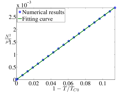
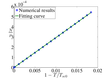
Tables 1 and 2 show that the ground state near zero temperature limit only depends on the sign of . These can be understood in a physical manner if we pay more attention to this phenomenological parameter in (150), where it was introduced to describe the self-interaction between the magnetic moments of complex vector field. The case of means that the p-wave pair will attract the one with the same magnetic moment direction and repulse the one with the opposite magnetic moment. Under the influence of spontaneous magnetization, the magnetic moment of p-wave pair will tend to align along the direction of spontaneous magnetization. As a result, p-wave pair and spontaneous magnetization would be enhanced by each other and therefore survive. However, if , the p-wave pair will repulse the one with the same magnetic moment direction. So the p-wave pair will align without net magnetism and the system is in a pure p-wave superconducting phase in the region where superconductivity dominates. When , the ferromagnetism can appear, which tends to make p-wave pairs have same direction. But the p-wave pairs with same magnetic moment direction will repulse each other, which leads that the p-wave pair is not stable and will be de-paired. So the system can only be in the ferromagnetic phase.
8 Conclusion and Discussion
Due to the strong/weak duality characteristic of the holographic correspondence, it provides us with a powerful tool to study the properties of strongly interacting systems by a weakly coupled gravity theory with one extra spatial dimension. Although the underlying dynamics which govern the dual field theory and the gravity are apparently different, as we have shown, in the framework of holography quantum computations in the dual (strongly coupled) field theory can be translated into classical calculations in the bulk, where one can just solve differential equations with suitable boundary conditions. Within this framework, holographic correspondence is considered as a hopeful approach to understand the properties of strongly correlated electron systems.
The bulk gravitational models that we have reviewed are some phenomenological models. In such bottom-up approach, the gravity duals were constructed using the minimal set of fields that captured the essential dynamics. They just involve gravity interacting with an effective U(1) gauge field and a charged field serving as the order parameter. We have a lot of the degrees of freedom to choose the form of interactions as well as the value of couplings.323232In principle, the arbitrary can be fixed by embedding the bulk model into some low energy effective theory of string/M theory. Nevertheless, one has seen that those simple models would describe dual superconductors rather well. Some interesting features have been uncovered. Let us take holographic p-wave models as an example. For the SU(2) Yang-Mills model (42), the conductivities are strongly anisotropic in a manner which is suggestive of a gap with nodes. The low-lying excitations of the normal state have a relaxation time growing rapidly as the temperature is lowered, which agrees with the absence of impurity scattering. For the second model (57), it has been found that the vector condensate can be induced by an applied magnetic field, and the condensation of the charged vector operator forms a vortex lattice structure in the spatial directions perpendicular to the magnetic field. Going beyond the probe approximation, the model displays a rich phase structure. In terms of temperature and chemical potential, the complete phase diagrams have been constructed for the conducting phase, insulating phase and their corresponding superconducting phases and some new phase boundaries are revealed. The Maxwell-vector model is a generalization of the SU(2) model in the sense that the vector field has a general mass and gyromagnetic ratio. The third model (76) realizes a p-wave superconducting phase by involving a charged two-form in the bulk. The p-wave states exhibit a helical structure and some of them display the phenomenon of pitch inversion as the temperature is decreased. The ground state of the condensed phase has zero entropy density and exhibits an emergent scaling symmetry in the IR.
It is clear that the key ingredient in constructing a gravitational dual of a superconductor is to find an instability which breaks a U(1) symmetry, e.g., at low temperatures and causes a condensate to form spontaneously. One may ask whether those phenomenological bulk duals of superconductors are just a Ginzburg-Landau description. The answer is exactly no. Let us stress two key differences. First, the instability in the Ginzburg-Landau model must be put in by hand, while it arises naturally in holographic setup. Second, the Ginzburg-Landau model is only valid near the transition point, whereas the gravitational description can characterize the whole dynamics. For a given bulk action, scanning through values of model parameters corresponds to scanning through many different dual field theories. In that sense, a simple holographic model has a kind of universality, i.e., the results may be true for a large class of dual field theories, quite insensitive to the details of their dynamics. Another confusion is that we realized the spontaneous breaking of a continuous U(1) symmetry in dimensions at finite temperature, in apparent contradiction to the Coleman-Mermin-Wagner theorem. The cure is that the large limit evades the theorem as fluctuations are suppressed. It would be interesting to discuss the effect of bulk quantum corrections which correspond to corrections in the dual field theory [157]. Finally, although the hair breaks a local U(1) symmetry in the bulk, according to the dictionary, the dual system consists of a condensate breaking a global U(1) symmetry. On the other hand, the onset of superconductivity is characterized by the condensation of a composite charged operator spontaneously breaking U(1) gauge symmetry. So strictly speaking, what one has realized is a dual theory of superfluid [158, 159, 160, 161] rather than superconductor. However, in the limit that the U(1) symmetry is “weakly gauged” one can still view the dual theory describing a superconductor. 333333In fact, most of the condensed matter theories do not include dynamical photons, as their effects are usually small. For example, in the BCS theory electromagnetic field is often introduced as an external field. The possibility of introducing dynamical gauge fields in holographic superconductors was discussed in refs. [162, 163].
Throughout this brief summary we have been mainly concerned with static and homogeneous case and focused on some basic aspects. This is a rapidly devolving field, due to the limitation of length, we are not able to give more details for many interesting developments, such as introduction of momentum dissipation (to break translational symmetry) [164, 165, 166, 167, 168, 169, 170, 171, 172], construction of holographic Josephson Junction [173, 174, 175, 176, 177, 178, 179, 180, 181, 182], and investigation on dynamics for far-from equilibrium state [183, 184, 185, 186, 187, 188, 189, 190, 191, 192]. The analysis for the most part has been done numerically. To explore the properties of holographic superconductors using analytical techniques can be found, for example, in refs. [193, 194, 195, 196, 197, 198, 199, 200, 201, 202, 203, 204]. Optimistically the growing literature based on holographic duality might shed some light on the understanding of mysterious phenomena and eventually microscopic origins of strongly correlated superconductivity.
The applications of the holographic correspondence are still going on. It was written by G. T. Horowitz and J. Polchinski [205] that we find it difficult to believe that nature does not make use of it, but the precise way in which it does so remains to be discovered. In addition to holographic superconductors, the holographic approach has been used to understand some other aspects of condensed matter physics, including (non-)Fermi liquids [206, 207, 208, 209, 210], quantum Hall effect [211, 212, 213], strange metals [214, 215, 216, 217], topological insulators [218, 219, 220], Hubbard model [221] and so on. A major application using holographic duality is to describe quantum chromodynamics (QCD), especially for the quark gluon plasma produced in particle accelerators. It is referred as AdS/QCD or holographic QCD, which has been widely studied [222, 223, 224, 225, 226, 227, 228, 229, 230, 231, 232, 233, 234, 235]. Another emerging subject is the fluid/gravity correspondence, which translates problems in fluid dynamics into problems in general relativity [236, 237, 238]. Readers who are interested in those exciting achievements are encouraged to consult those relevant references.
Acknowledgements
This work was supported in part by the National Natural Science Foundation of China ( No.11035008, No.11375247, No.11205226 and No.11435006 ). L Li was supported in part by European Union’s Seventh Framework Programme under grant agreements (FP7-REGPOT-2012-2013-1) no 316165, the EU-Greece program “Thales” MIS 375734 and was also co-financed by the European Union (European Social Fund, ESF) and Greek national funds through the Operational Program “Education and Lifelong Learning” of the National Strategic Reference Framework (NSRF) under “Funding of proposals that have received a positive evaluation in the 3rd and 4th Call of ERC Grant Schemes”.
References
- [1] J. Bardeen, L. N. Cooper and J. R. Schrieffer, “Theory Of Superconductivity,” Phys. Rev. 108, 1175 (1957).
- [2] E. W. Carlson, V. J. Emery, S. A. Kivelson and D. Orgad, “Concepts in High Temperature Superconductivity,” [arXiv:cond-mat/0206217].
- [3] J. M. Maldacena, “The large N limit of superconformal field theories and supergravity,” Adv. Theor. Math. Phys. 2, 231 (1998) [Int. J. Theor. Phys. 38, 1113 (1999)] [arXiv:hep-th/9711200].
- [4] S. S. Gubser, I. R. Klebanov and A. M. Polyakov, “Gauge theory correlators from non-critical string theory,” Phys. Lett. B 428, 105 (1998) [arXiv:hep-th/9802109].
- [5] E. Witten, “Anti-de Sitter space and holography,” Adv. Theor. Math. Phys. 2, 253 (1998) [arXiv:hep-th/9802150].
- [6] X. L. Qi, “Exact holographic mapping and emergent space-time geometry,” arXiv:1309.6282 [hep-th].
- [7] G. T. Horowitz, “Introduction to Holographic Superconductors,” Lect. Notes Phys. 828, 313 (2011) [arXiv:1002.1722 [hep-th]].
- [8] C. P. Herzog, “Lectures on Holographic Superfluidity and Superconductivity,” J. Phys. A 42, 343001 (2009) [arXiv:0904.1975 [hep-th]].
- [9] N. Iqbal, H. Liu and M. Mezei, “Lectures on holographic non-Fermi liquids and quantum phase transitions,” arXiv:1110.3814 [hep-th].
- [10] D. Musso, “Introductory notes on holographic superconductors,” arXiv:1401.1504 [hep-th].
- [11] S. A. Hartnoll, C. P. Herzog and G. T. Horowitz, “Building a Holographic Superconductor,” Phys. Rev. Lett. 101, 031601 (2008) [arXiv:0803.3295 [hep-th]].
- [12] S. A. Hartnoll, C. P. Herzog and G. T. Horowitz, “Holographic Superconductors,” JHEP 0812, 015 (2008) [arXiv:0810.1563 [hep-th]].
- [13] T. Nishioka, S. Ryu and T. Takayanagi, “Holographic Superconductor/Insulator Transition at Zero Temperature,” JHEP 1003, 131 (2010) [arXiv:0911.0962 [hep-th]].
- [14] J. -W. Chen, Y. -J. Kao, D. Maity, W. -Y. Wen and C. -P. Yeh, “Towards A Holographic Model of D-Wave Superconductors,” Phys. Rev. D 81, 106008 (2010) [arXiv:1003.2991 [hep-th]].
- [15] F. Benini, C. P. Herzog, R. Rahman and A. Yarom, “Gauge gravity duality for d-wave superconductors: prospects and challenges,” JHEP 1011, 137 (2010) [arXiv:1007.1981 [hep-th]].
- [16] A. P. Mackenzie and Y. Maeno, “p-wave superconductivity,” Physica. B 280, 148-153 (2000).
- [17] S. S. Gubser and S. S. Pufu, “The Gravity dual of a p-wave superconductor,” JHEP 0811, 033 (2008) [arXiv:0805.2960 [hep-th]].
- [18] R. G. Cai, S. He, L. Li and L. F. Li, “A Holographic Study on Vector Condensate Induced by a Magnetic Field,” JHEP 1312, 036 (2013) [arXiv:1309.2098 [hep-th]].
- [19] R. -G. Cai, L. Li and L. -F. Li, “A Holographic P-wave Superconductor Model,” JHEP 1401, 032 (2014) [arXiv:1309.4877 [hep-th]].
- [20] F. Aprile, D. Rodriguez-Gomez and J. G. Russo, “p-wave Holographic Superconductors and five-dimensional gauged Supergravity,” JHEP 1101, 056 (2011) [arXiv:1011.2172 [hep-th]].
- [21] A. Donos and J. P. Gauntlett, “Holographic helical superconductors,” JHEP 1112, 091 (2011) [arXiv:1109.3866 [hep-th]].
- [22] A. Donos and J. P. Gauntlett, “Helical superconducting black holes,” Phys. Rev. Lett. 108, 211601 (2012) [arXiv:1203.0533 [hep-th]].
- [23] F. Denef and S. A. Hartnoll, “Landscape of superconducting membranes,” Phys. Rev. D 79, 126008 (2009) [arXiv:0901.1160 [hep-th]].
- [24] S. S. Gubser, C. P. Herzog, S. S. Pufu and T. Tesileanu, “Superconductors from Superstrings,” Phys. Rev. Lett. 103, 141601 (2009) [arXiv:0907.3510 [hep-th]].
- [25] J. P. Gauntlett, J. Sonner and T. Wiseman, “Holographic superconductivity in M-Theory,” Phys. Rev. Lett. 103, 151601 (2009) [arXiv:0907.3796 [hep-th]].
- [26] S. S. Gubser, S. S. Pufu and F. D. Rocha, “Quantum critical superconductors in string theory and M-theory,” Phys. Lett. B 683, 201 (2010) [arXiv:0908.0011 [hep-th]].
- [27] J. P. Gauntlett, J. Sonner and T. Wiseman, “Quantum Criticality and Holographic Superconductors in M-theory,” JHEP 1002, 060 (2010) [arXiv:0912.0512 [hep-th]].
- [28] S. Kalyana Rama, S. Sarkar, B. Sathiapalan and N. Sircar, “Strong Coupling BCS Superconductivity and Holography,” Nucl. Phys. B 852, 634 (2011) [arXiv:1104.2843 [hep-th]].
- [29] N. Bobev, A. Kundu, K. Pilch and N. P. Warner, “Minimal Holographic Superconductors from Maximal Supergravity,” JHEP 1203, 064 (2012) [arXiv:1110.3454 [hep-th]].
- [30] V. L. Ginzburg and L. D. Landau, “On the Theory of superconductivity,” Zh. Eksp. Teor. Fiz. 20, 1064 (1950).
- [31] M. Cyrot, “Ginzburg-Landau theory for superconductors”, Rep. Prog. Phys. 36, 103 (1973).
- [32] S. Weinberg, “Superconductivity for Particular Theorists,” Progress of Theoretical Physics Supplement, 86, 43 (1986).
- [33] S. Kachru, X. Liu and M. Mulligan, “Gravity duals of Lifshitz-like fixed points,” Phys. Rev. D 78, 106005 (2008) [arXiv:0808.1725 [hep-th]].
- [34] D. T. Son, “Toward an AdS/cold atoms correspondence: A Geometric realization of the Schrodinger symmetry,” Phys. Rev. D 78, 046003 (2008) [arXiv:0804.3972 [hep-th]].
- [35] K. Balasubramanian and J. McGreevy, “Gravity duals for non-relativistic CFTs,” Phys. Rev. Lett. 101, 061601 (2008) [arXiv:0804.4053 [hep-th]].
- [36] C. Charmousis, B. Gouteraux, B. S. Kim, E. Kiritsis and R. Meyer, “Effective Holographic Theories for low-temperature condensed matter systems,” JHEP 1011, 151 (2010) [arXiv:1005.4690 [hep-th]].
- [37] B. Gouteraux and E. Kiritsis, “Generalized Holographic Quantum Criticality at Finite Density,” JHEP 1112, 036 (2011) [arXiv:1107.2116 [hep-th]].
- [38] L. Huijse, S. Sachdev and B. Swingle, “Hidden Fermi surfaces in compressible states of gauge-gravity duality,” Phys. Rev. B 85, 035121 (2012) [arXiv:1112.0573 [cond-mat.str-el]].
- [39] X. Dong, S. Harrison, S. Kachru, G. Torroba and H. Wang, “Aspects of holography for theories with hyperscaling violation,” JHEP 1206, 041 (2012) [arXiv:1201.1905 [hep-th]].
- [40] B. S. Kim, “Schródinger Holography with and without Hyperscaling Violation,” JHEP 1206, 116 (2012) [arXiv:1202.6062 [hep-th]].
- [41] P. Breitenlohner and D. Z. Freedman, “Stability in Gauged Extended Supergravity,” Annals Phys. 144, 249 (1982).
- [42] A. W. Peet and J. Polchinski, “UV / IR relations in AdS dynamics,” Phys. Rev. D 59, 065011 (1999) [hep-th/9809022].
- [43] V. Balasubramanian and P. Kraus, “A Stress tensor for Anti-de Sitter gravity,” Commun. Math. Phys. 208, 413 (1999) [hep-th/9902121].
- [44] M. Bianchi, D. Z. Freedman and K. Skenderis, “How to go with an RG flow,” JHEP 0108, 041 (2001) [hep-th/0105276].
- [45] M. Bianchi, D. Z. Freedman and K. Skenderis, “Holographic renormalization,” Nucl. Phys. B 631, 159 (2002) [hep-th/0112119].
- [46] D. T. Son and A. O. Starinets, “Minkowski space correlators in AdS/CFT correspondence: Recipe and applications,” JHEP 0209, 042 (2002) [hep-th/0205051].
- [47] C. P. Herzog and D. T. Son, “Schwinger-Keldysh propagators from AdS/CFT correspondence,” JHEP 0303, 046 (2003) [hep-th/0212072].
- [48] K. Skenderis and B. C. van Rees, “Real-time gauge/gravity duality,” Phys. Rev. Lett. 101, 081601 (2008) [arXiv:0805.0150 [hep-th]].
- [49] I. R. Klebanov and E. Witten, “AdS / CFT correspondence and symmetry breaking,” Nucl. Phys. B 556, 89 (1999) [hep-th/9905104].
- [50] E. Witten, “Multitrace operators, boundary conditions, and AdS / CFT correspondence,” hep-th/0112258.
- [51] M. Berkooz, A. Sever and A. Shomer, “’Double trace’ deformations, boundary conditions and space-time singularities,” JHEP 0205, 034 (2002) [hep-th/0112264].
- [52] S. W. Hawking, “Breakdown of Predictability in Gravitational Collapse,” Phys. Rev. D 14, 2460 (1976).
- [53] S. W. Hawking, “Information loss in black holes,” Phys. Rev. D 72, 084013 (2005) [hep-th/0507171].
- [54] S. W. Hawking, “Information Preservation and Weather Forecasting for Black Holes,” arXiv:1401.5761 [hep-th].
- [55] O. Aharony, S. S. Gubser, J. M. Maldacena, H. Ooguri and Y. Oz, “Large N field theories, string theory and gravity,” Phys. Rept. 323, 183 (2000) [hep-th/9905111].
- [56] S. A. Hartnoll, “Lectures on holographic methods for condensed matter physics,” Class. Quant. Grav. 26, 224002 (2009) [arXiv:0903.3246 [hep-th]].
- [57] J. McGreevy, “Holographic duality with a view toward many-body physics,” Adv. High Energy Phys. 2010, 723105 (2010) [arXiv:0909.0518 [hep-th]].
- [58] J. Casalderrey-Solana, H. Liu, D. Mateos, K. Rajagopal and U. A. Wiedemann, “Gauge/String Duality, Hot QCD and Heavy Ion Collisions,” arXiv:1101.0618 [hep-th].
- [59] A. Adams, L. D. Carr, T. Sch fer, P. Steinberg and J. E. Thomas, “Strongly Correlated Quantum Fluids: Ultracold Quantum Gases, Quantum Chromodynamic Plasmas, and Holographic Duality,” New J. Phys. 14, 115009 (2012) [arXiv:1205.5180 [hep-th]].
- [60] S. Sachdev, “What can gauge-gravity duality teach us about condensed matter physics?,” Ann. Rev. Condensed Matter Phys. 3, 9 (2012) [arXiv:1108.1197 [cond-mat.str-el]].
- [61] S. Franco, A. Garcia-Garcia and D. Rodriguez-Gomez, “A General class of holographic superconductors,” JHEP 1004, 092 (2010) [arXiv:0906.1214 [hep-th]].
- [62] F. Aprile and J. G. Russo, “Models of Holographic superconductivity,” Phys. Rev. D 81, 026009 (2010) [arXiv:0912.0480 [hep-th]].
- [63] F. Aprile, S. Franco, D. Rodriguez-Gomez and J. G. Russo, “Phenomenological Models of Holographic Superconductors and Hall currents,” JHEP 1005, 102 (2010) [arXiv:1003.4487 [hep-th]].
- [64] Y. Liu and Y. W. Sun, “Holographic Superconductors from Einstein-Maxwell-Dilaton Gravity,” JHEP 1007, 099 (2010) [arXiv:1006.2726 [hep-th]].
- [65] S. Chen, Q. Pan and J. Jing, “Holographic superconductor models in the non-minimal derivative coupling theory,” Chin. Phys. B 21, 040403 (2012) [arXiv:1012.3820 [gr-qc]].
- [66] Y. Peng, Q. Pan and B. Wang, “Various types of phase transitions in the AdS soliton background,” Phys. Lett. B 699, 383 (2011) [arXiv:1104.2478 [hep-th]].
- [67] F. Bigazzi, A. L. Cotrone, D. Musso, N. P. Fokeeva and D. Seminara, “Unbalanced Holographic Superconductors and Spintronics,” JHEP 1202, 078 (2012) [arXiv:1111.6601 [hep-th]].
- [68] A. Dey, S. Mahapatra and T. Sarkar, “Generalized Holographic Superconductors with Higher Derivative Couplings,” JHEP 1406, 147 (2014) [arXiv:1404.2190 [hep-th]].
- [69] D. Arean and J. Tarrio, “Bifundamental Superfluids from Holography,” arXiv:1501.02804 [hep-th].
- [70] S. S. Gubser, “Breaking an Abelian gauge symmetry near a black hole horizon,” Phys. Rev. D 78, 065034 (2008) [arXiv:0801.2977 [hep-th]].
- [71] T. Faulkner, G. T. Horowitz and M. M. Roberts, “Holographic quantum criticality from multi-trace deformations,” JHEP 1104, 051 (2011) [arXiv:1008.1581 [hep-th]].
- [72] G. T. Horowitz and M. M. Roberts, “Holographic Superconductors with Various Condensates,” Phys. Rev. D 78, 126008 (2008) [arXiv:0810.1077 [hep-th]].
- [73] G. T. Horowitz and M. M. Roberts, “Zero Temperature Limit of Holographic Superconductors,” JHEP 0911, 015 (2009) [arXiv:0908.3677 [hep-th]].
- [74] K. Maeda and T. Okamura, “Characteristic length of an AdS/CFT superconductor,” Phys. Rev. D 78, 106006 (2008) [arXiv:0809.3079 [hep-th]].
- [75] K. Maeda, M. Natsuume and T. Okamura, “Vortex lattice for a holographic superconductor,” Phys. Rev. D 81, 026002 (2010) [arXiv:0910.4475 [hep-th]].
- [76] T. Faulkner, G. T. Horowitz, J. McGreevy, M. M. Roberts and D. Vegh, “Photoemission ‘experiments’ on holographic superconductors,” JHEP 1003, 121 (2010) [arXiv:0911.3402 [hep-th]].
- [77] A. Bagrov, B. Meszena and K. Schalm, “Pairing induced superconductivity in holography,” JHEP 1409, 106 (2014) [arXiv:1403.3699 [hep-th]].
- [78] G. T. Horowitz and B. Way, “Complete Phase Diagrams for a Holographic Superconductor/Insulator System,” JHEP 1011, 011 (2010) [arXiv:1007.3714 [hep-th]].
- [79] R. G. Cai, S. He, L. Li and Y. L. Zhang, “Holographic Entanglement Entropy in Insulator/Superconductor Transition,” JHEP 1207, 088 (2012) [arXiv:1203.6620 [hep-th]].
- [80] R. G. Cai, S. He, L. Li and L. F. Li, “Entanglement Entropy and Wilson Loop in Stúckelberg Holographic Insulator/Superconductor Model,” JHEP 1210, 107 (2012) [arXiv:1209.1019 [hep-th]].
- [81] W. Yao and J. Jing, “Holographic entanglement entropy in insulator/superconductor transition with Born-Infeld electrodynamics,” JHEP 1405, 058 (2014) [arXiv:1401.6505 [hep-th]].
- [82] P. Basu, J. He, A. Mukherjee and H. H. Shieh, “Hard-gapped Holographic Superconductors,” Phys. Lett. B 689, 45 (2010) [arXiv:0911.4999 [hep-th]].
- [83] M. M. Roberts and S. A. Hartnoll, “Pseudogap and time reversal breaking in a holographic superconductor,” JHEP 0808, 035 (2008) [arXiv:0805.3898 [hep-th]].
- [84] A. Akhavan and M. Alishahiha, “P-Wave Holographic Insulator/Superconductor Phase Transition,” Phys. Rev. D 83, 086003 (2011) [arXiv:1011.6158 [hep-th]].
- [85] M. Ammon, J. Erdmenger, P. Kerner and M. Strydom, “Black Hole Instability Induced by a Magnetic Field,” Phys. Lett. B 706, 94 (2011) [arXiv:1106.4551 [hep-th]].
- [86] Y. -Y. Bu, J. Erdmenger, J. P. Shock and M. Strydom, “Magnetic field induced lattice ground states from holography,” JHEP 1303, 165 (2013) [arXiv:1210.6669 [hep-th]].
- [87] M. Ammon, J. Erdmenger, M. Kaminski and P. Kerner, “Superconductivity from gauge/gravity duality with flavor,” Phys. Lett. B 680, 516 (2009) [arXiv:0810.2316 [hep-th]].
- [88] P. Basu, J. He, A. Mukherjee and H. -H. Shieh, “Superconductivity from D3/D7: Holographic Pion Superfluid,” JHEP 0911, 070 (2009) [arXiv:0810.3970 [hep-th]].
- [89] M. Ammon, J. Erdmenger, M. Kaminski and P. Kerner, “Flavor Superconductivity from Gauge/Gravity Duality,” JHEP 0910, 067 (2009) [arXiv:0903.1864 [hep-th]].
- [90] M. Ammon, J. Erdmenger, V. Grass, P. Kerner and A. O’Bannon, “On Holographic p-wave Superfluids with Back-reaction,” Phys. Lett. B 686, 192 (2010) [arXiv:0912.3515 [hep-th]].
- [91] R. -G. Cai, Z. -Y. Nie and H. -Q. Zhang, “Holographic Phase Transitions of P-wave Superconductors in Gauss-Bonnet Gravity with Back-reaction,” Phys. Rev. D 83, 066013 (2011) [arXiv:1012.5559 [hep-th]].
- [92] R. -G. Cai, Z. -Y. Nie and H. -Q. Zhang, “Holographic p-wave superconductors from Gauss-Bonnet gravity,” Phys. Rev. D 82, 066007 (2010) [arXiv:1007.3321 [hep-th]].
- [93] L. A. Pando Zayas and D. Reichmann, “A Holographic Chiral Superconductor,” Phys. Rev. D 85, 106012 (2012) [arXiv:1108.4022 [hep-th]].
- [94] R. -G. Cai, S. He, L. Li and Y. -L. Zhang, “Holographic Entanglement Entropy on P-wave Superconductor Phase Transition,” JHEP 1207, 027 (2012) [arXiv:1204.5962 [hep-th]].
- [95] R. E. Arias and I. S. Landea, “Backreacting p-wave Superconductors,” JHEP 1301, 157 (2013) [arXiv:1210.6823 [hep-th]].
- [96] R. -G. Cai, L. Li, L. -F. Li and R. -K. Su, “Entanglement Entropy in Holographic P-Wave Superconductor/Insulator Model,” JHEP 1306, 063 (2013) [arXiv:1303.4828 [hep-th]].
- [97] D. Djukanovic, M. R. Schindler, J. Gegelia and S. Scherer, “Quantum electrodynamics for vector mesons,” Phys. Rev. Lett. 95, 012001 (2005) [hep-ph/0505180].
- [98] J. A. Young and S. A. Bludman, “Electromagnetic Properties of a Charged Vector Meson,” Phys. Rev. 131, 2326 (1963).
- [99] Rasolt. Mark, “Superconductivity in high magnetic fields,” Phys. Rev. Lett. 58, 1482 (1987).
- [100] M. Rasolt and Z. Tesanovic, “Theoretical aspects of superconductivity in very high magnetic fields,” Rev. Mod. Phys. 64, 709 (1992).
- [101] F. Levy, I. Sheikin, B. Grenier, A. Huxley, “Magnetic Field-induced Superconductivity in the Ferromagnet URhGe,” Science 309 1343 (2005).
- [102] S. Uji, H. Shinagawa, T. Terashima, T. Yakabe, Y. Teral, M. Tokumoto, A. Kobayashi, H. Tanaka, H. Kobayashi, “Magnetic-field-induced superconductivity in a two-dimensional organic conductor,” Nature 410 908 (2010).
- [103] R. G. Cai, L. Li, L. F. Li and Y. Wu, “Vector Condensate and AdS Soliton Instability Induced by a Magnetic Field,” JHEP 1401, 045 (2014) [arXiv:1311.7578 [hep-th]].
- [104] M. N. Chernodub, “Superconductivity of QCD vacuum in strong magnetic field,” Phys. Rev. D 82, 085011 (2010) [arXiv:1008.1055 [hep-ph]].
- [105] M. N. Chernodub, “Spontaneous electromagnetic superconductivity of vacuum in strong magnetic field: evidence from the Nambu–Jona-Lasinio model,” Phys. Rev. Lett. 106, 142003 (2011) [arXiv:1101.0117 [hep-ph]].
- [106] R. -G. Cai, L. Li, L. -F. Li and R. -Q. Yang, “Towards Complete Phase Diagrams of a Holographic P-wave Superconductor Model,” JHEP 1404, 016 (2014) [arXiv:1401.3974 [gr-qc]].
- [107] V. P. Maslov, “Zeroth-Order Phase Transitions,” Mathematical Notes 76, 697 (2004).
- [108] H. B. Zeng, “Possible Anderson localization in a holographic superconductor,” Phys. Rev. D 88, 126004 (2013) [arXiv:1310.5753 [hep-th]].
- [109] H. B. Zeng and H. Q. Zhang, “Zeroth Order Phase Transition in a Holographic Superconductor with Single Impurity,” arXiv:1411.3955 [hep-th].
- [110] P. Chaturvedi and G. Sengupta, “p-wave Holographic Superconductors from Born-Infeld Black Holes,” arXiv:1501.06998 [hep-th].
- [111] A. A. Kordyuk, “Iron-based superconductors: Magnetism, superconductivity, and electronic structure,” Low. Temp. Phys. 38, 888 (2012).
- [112] A. Chubukov, “Pairing Mechanism in Fe-Based Superconductors,” Annu. Rev. Condens. Matter Phys. 3, 357 (2012).
- [113] H. Q. Yuan et al., “Observation of Two Distinct Superconducting Phases in CeCu2Si2,” Science 302, 2104 (2003).
- [114] P. Fulde and R. A. Ferrell, “Superconductivity in a Strong Spin-Exchange Field,” Phys. Rev. 135, A550 (1964).
- [115] A. I. larkin and Y. N. Ovchinnikov, “Nonuniform state of superconductors,” Zh. Eksp. Teor. Fiz. 47, 1136 (1964) [Sov. Phys. JETP 20, 762 (1965)].
- [116] A. Donos, J. P. Gauntlett and C. Pantelidou, “Competing p-wave orders,” Class. Quant. Grav. 31, 055007 (2014) [arXiv:1310.5741 [hep-th]].
- [117] P. J. Hirschfeld, W. O. Putikka and D. J. Scalapino, “Microwave conductivity of d-wave superconductors,” Phys. Rev. Lett. 71, 3705 (1993).
- [118] F. Benini, C. P. Herzog and A. Yarom, “Holographic Fermi arcs and a d-wave gap,” Phys. Lett. B 701, 626 (2011) [arXiv:1006.0731 [hep-th]].
- [119] J. W. Chen, Y. S. Liu and D. Maity, “ Holographic Superconductors,” JHEP 1105, 032 (2011) [arXiv:1103.1714 [hep-th]].
- [120] K. -Y. Kim and M. Taylor, “Holographic d-wave superconductors,” JHEP 1308, 112 (2013) [arXiv:1304.6729 [hep-th]].
- [121] M. R. Norman “The Challenge of Unconventional Superconductivity,” Science 332, 196 (2011).
- [122] E. Berg, E. Fradkin, S. A. Kivelson and J. M. Tranquada, “Striped superconductors: how spin, charge and superconducting orders intertwine in the cuprates,” New J. Phys. 11, 115004 (2009).
- [123] J. Zaanen, “A Modern, but way too short history of the theory of superconductivity at a high temperature,” [arXiv:1012.5461 [cond-mat.supr-con]].
- [124] R. G. Cai, L. Li, L. F. Li and Y. Q. Wang, “Competition and Coexistence of Order Parameters in Holographic Multi-Band Superconductors,” JHEP 1309, 074 (2013) [arXiv:1307.2768 [hep-th]].
- [125] Z. Y. Nie, R. G. Cai, X. Gao and H. Zeng, “Competition between the s-wave and p-wave superconductivity phases in a holographic model,” JHEP 1311, 087 (2013) [arXiv:1309.2204 [hep-th]].
- [126] I. Amado, D. Arean, A. Jimenez-Alba, L. Melgar and I. Salazar Landea, “Holographic s+p Superconductors,” Phys. Rev. D 89, 026009 (2014) [arXiv:1309.5086 [hep-th]].
- [127] L. F. Li, R. G. Cai, L. Li and Y. Q. Wang, “Competition between s-wave order and d-wave order in holographic superconductors,” JHEP 1408, 164 (2014) [arXiv:1405.0382 [hep-th]].
- [128] M. Nishida, “Phase Diagram of a Holographic Superconductor Model with s-wave and d-wave,” JHEP 1409, 154 (2014) [arXiv:1403.6070 [hep-th]].
- [129] P. Basu, J. He, A. Mukherjee, M. Rozali and H. -H. Shieh, “Competing Holographic Orders,” JHEP 1010, 092 (2010) [arXiv:1007.3480 [hep-th]].
- [130] D. Musso, “Competition/Enhancement of Two Probe Order Parameters in the Unbalanced Holographic Superconductor,” JHEP 1306, 083 (2013) [arXiv:1302.7205 [hep-th]].
- [131] Y. Liu, K. Schalm, Y. W. Sun and J. Zaanen, “Bose-Fermi competition in holographic metals,” JHEP 1310, 064 (2013) [arXiv:1307.4572 [hep-th]].
- [132] A. Amoretti, A. Braggio, N. Maggiore, N. Magnoli and D. Musso, “Coexistence of two vector order parameters: a holographic model for ferromagnetic superconductivity,” JHEP 1401, 054 (2014) [arXiv:1309.5093 [hep-th]].
- [133] W. Y. Wen, M. S. Wu and S. Y. Wu, “A Holographic Model of Two-Band Superconductor,” Phys. Rev. D 89, 066005 (2014) [arXiv:1309.0488 [hep-th]].
- [134] A. Donos, J. P. Gauntlett, J. Sonner and B. Withers, “Competing orders in M-theory: superfluids, stripes and metamagnetism,” JHEP 1303, 108 (2013) [arXiv:1212.0871 [hep-th]].
- [135] M. Silaev and E. Babaev, “Microscopic derivation of two-component Ginzburg-Landau model and conditions of its applicability in two-band systems,” Phys. Rev. B 85, 134514 (2012) [arXiv:1110.1593 [cond-mat]].
- [136] A. A. Shanenko, M. V. Milošević, F. M. Peeters and A. V. Vagov, “Extended Ginzburg-Landau Formalism for Two-Band Superconductors,” Phys. Rev. Lett. 106, 047005 (2011) [arXiv:1101.0971 [cond-mat.supr-con]].
- [137] A. Vagov, A. A. Shanenko, M. V. Milošević, V. M. Axt, and F. M. Peeters, “Two-band superconductors: Extended Ginzburg-Landau formalism by a systematic expansion in small deviation from the critical temperature,” Phys. Rev. B 86, 144514 (2012) [arXiv:1207.6297 [cond-mat.supr-con]].
- [138] J. Carlstrom, E. Babaev and M. Speight, “Type-1.5 superconductivity in multiband systems: Effects of interband couplings,” Phys. Rev. B 83, 174509 (2011) [arXiv:1009.2196 [cond-mat.supr-con]].
- [139] C. Buzea and T. Yamashita, “Review of superconducting properties of MgB2,” Superconductors, Science & Technology, Vol. 14, No. 11 (2001) R115-R146 [arXiv:cond-mat/0108265 [cond-mat.supr-con]].
- [140] P. J. Hirschfeld, M. M. Korshunov and I. I. Mazin, “Gap symmetry and structure of Fe-based superconductors,” Rep. Prog. Phys. 74, 124508 (2011) [arXiv:1106.3712 [cond-mat.supr-con]].
- [141] David C. Johnston, “The Puzzle of High Temperature Superconductivity in Layered Iron Pnictides and Chalcogenides,” Advances in Physics 59, 803-1061 (2010) [arXiv:1005.4392 [cond-mat.supr-con]].
- [142] G. R. Stewart, “Superconductivity in Iron Compounds,” Rev. Mod. Phys. 83 1589-1652 (2011) [arXiv:1106.1618 [cond-mat.supr-con]].
- [143] Z. Y. Nie, R. G. Cai, X. Gao, L. Li and H. Zeng, “Phase transitions in a holographic s+p model with backreaction,” arXiv:1501.00004 [hep-th].
- [144] P. Goswami, B. Roy, “Axionic superconductivity in three dimensional doped narrow gap semiconductors,” Phys. Rev. B 90, 041301(R)(2014) [arXiv:1307.3240 [cond-mat.supr-con]].
- [145] G. G. Lonzarich, S. S. Saxena, P. Agarwal, K. Ahilan, F. M. Grosche, R. K. W. Haselwimmer, M. J. Steiner, E. Pugh, et al., “Superconductivity on the border of itinerant-electron ferromagnetism in UGe2,” Nature 406 587 (2000).
- [146] D. Aoki, A. Huxley, E. Ressouche, D. Braithwaite, J. Flouquet, J-P. Brison, E. Lhotel and C. Paulsen, “Coexistence of superconductivity and ferromagnetism in URhGe,” Nature 413 613 (2001).
- [147] N. T. Huy, A. Gasparini, et al., “Superconductivity on the border of weak itinerant ferromagnetism in UCoGe,” Phys. Rev. Lett. 99, 067006 (2007).
- [148] C. Pfleiderer, M. Uhlarz, S. M. Hayden, R. Vollmer, H. Lohneysen, N. Bernhoeft and G. Lonzarich, “ Coexistence of superconductivity and ferromagnetism in the d-band metal ZrZn2,” Nature 412, 58 (2001).
- [149] D. I. Uzunov, “Theory of ferromagnetic unconventional superconductors with spin-triplet electron pairing,” [arXiv:1204.1007v2[cond-mat]].
- [150] K. Machida, T. Ohmi, “Theory of Ferromagnetic Superconductivity,” Phys. Rev. Lett 86, 850 (2001) [arXiv:cond-mat/0008245].
- [151] Nevidomskyy H. Andriy, “Coexistence of Ferromagnetism and Superconductivity Close to a Quantum Phase Transition: The Heisenberg- to Ising-type Crossover,” Phys. Rev. Lett. 94,097003 (2005) [arXiv:cond-mat/0412247].
- [152] N. Iqbal, H. Liu, M. Mezei and Q. Si, “Quantum phase transitions in holographic models of magnetism and superconductors,” Phys. Rev. D 82, 045002 (2010) [arXiv:1003.0010 [hep-th]].
- [153] R. -G. Cai and R. -Q. Yang, “Paramagnetism-Ferromagnetism Phase Transition in a Dyonic Black Hole,” Phys. Rev. D 90, 081901 (2014) [arXiv:1404.2856 [hep-th]].
- [154] R. G. Cai and R. Q. Yang, “Coexistence and competition of ferromagnetism and -wave superconductivity in holographic model,” Phys. Rev. D 91, no. 2, 026001 (2015) [arXiv:1410.5080 [hep-th]].
- [155] R. G. Cai, R. Q. Yang and F. V. Kusmartsev, “A holographic model for antiferromagnetic quantum phase transition induced by magnetic field,” arXiv:1501.04481 [hep-th].
- [156] R. -G. Cai and Y. -Z. Zhang, “Black plane solutions in four-dimensional space-times,” Phys. Rev. D 54, 4891 (1996) [gr-qc/9609065].
- [157] D. Anninos, S. A. Hartnoll and N. Iqbal, “Holography and the Coleman-Mermin-Wagner theorem,” Phys. Rev. D 82, 066008 (2010) [arXiv:1005.1973 [hep-th]].
- [158] C. P. Herzog, P. K. Kovtun and D. T. Son, “Holographic model of superfluidity,” Phys. Rev. D 79, 066002 (2009) [arXiv:0809.4870 [hep-th]].
- [159] Y. Brihaye and B. Hartmann, “Holographic superfluid/fluid/insulator phase transitions in 2+1 dimensions,” Phys. Rev. D 83, 126008 (2011) [arXiv:1101.5708 [hep-th]].
- [160] D. Arean, M. Bertolini, C. Krishnan and T. Prochazka, “Type IIB Holographic Superfluid Flows,” JHEP 1103, 008 (2011) [arXiv:1010.5777 [hep-th]].
- [161] Y. B. Wu, J. W. Lu, W. X. Zhang, C. Y. Zhang, J. B. Lu and F. Yu, “Holographic -wave superfluid,” Phys. Rev. D 90, no. 12, 126006 (2014) [arXiv:1410.5243 [hep-th]].
- [162] O. Domenech, M. Montull, A. Pomarol, A. Salvio and P. J. Silva, “Emergent Gauge Fields in Holographic Superconductors,” JHEP 1008, 033 (2010) [arXiv:1005.1776 [hep-th]].
- [163] X. Gao, M. Kaminski, H. B. Zeng and H. Q. Zhang, “Non-Equilibrium Field Dynamics of an Honest Holographic Superconductor,” JHEP 1211, 112 (2012) [arXiv:1204.3103 [hep-th]].
- [164] R. Flauger, E. Pajer and S. Papanikolaou, “A Striped Holographic Superconductor,” Phys. Rev. D 83, 064009 (2011) [arXiv:1010.1775 [hep-th]].
- [165] G. T. Horowitz and J. E. Santos, “General Relativity and the Cuprates,” arXiv:1302.6586 [hep-th].
- [166] Ó. J. C. Dias, G. T. Horowitz, N. Iqbal and J. E. Santos, “Vortices in holographic superfluids and superconductors as conformal defects,” JHEP 1404, 096 (2014) [arXiv:1311.3673 [hep-th]].
- [167] H. B. Zeng and J. P. Wu, “Holographic superconductors from the massive gravity,” Phys. Rev. D 90, 046001 (2014) [arXiv:1404.5321 [hep-th]].
- [168] J. i. Koga, K. Maeda and K. Tomoda, “Holographic superconductor model in a spatially anisotropic background,” Phys. Rev. D 89, no. 10, 104024 (2014) [arXiv:1401.6501 [hep-th]].
- [169] Y. Ling, P. Liu, C. Niu, J. P. Wu and Z. Y. Xian, “Holographic Superconductor on Q-lattice,” arXiv:1410.6761 [hep-th].
- [170] D. Arean, A. Farahi, L. A. Pando Zayas, I. S. Landea and A. Scardicchio, “Holographic superconductor with disorder,” Phys. Rev. D 89, no. 10, 106003 (2014) [arXiv:1308.1920 [hep-th]].
- [171] J. Erdmenger, B. Herwerth, S. Klug, R. Meyer and K. Schalm, “S-Wave Superconductivity in Anisotropic Holographic Insulators,” arXiv:1501.07615 [hep-th].
- [172] K. Y. Kim, K. K. Kim and M. Park, “A Simple Holographic Superconductor with Momentum Relaxation,” arXiv:1501.00446 [hep-th].
- [173] G. T. Horowitz, J. E. Santos and B. Way, “A Holographic Josephson Junction,” Phys. Rev. Lett. 106, 221601 (2011) [arXiv:1101.3326 [hep-th]].
- [174] Y. Q. Wang, Y. X. Liu and Z. H. Zhao, “Holographic Josephson Junction in 3+1 dimensions,” arXiv:1104.4303 [hep-th].
- [175] M. Siani, “On inhomogeneous holographic superconductors,” arXiv:1104.4463 [hep-th].
- [176] Y. Q. Wang, Y. X. Liu and Z. H. Zhao, “Holographic p-wave Josephson junction,” arXiv:1109.4426 [hep-th].
- [177] Y. Q. Wang, Y. X. Liu, R. G. Cai, S. Takeuchi and H. Q. Zhang, “Holographic SIS Josephson Junction,” JHEP 1209, 058 (2012) [arXiv:1205.4406 [hep-th]].
- [178] M. Rozali and A. Vincart-Emard, “Chiral Edge Currents in a Holographic Josephson Junction,” JHEP 1401, 003 (2014) [arXiv:1310.4510 [hep-th]].
- [179] R. G. Cai, Y. Q. Wang and H. Q. Zhang, “A holographic model of SQUID,” JHEP 1401, 039 (2014) [arXiv:1308.5088 [hep-th]].
- [180] S. Takeuchi, “Holographic Superconducting Quantum Interference Device,” arXiv:1309.5641 [hep-th].
- [181] E. Kiritsis and V. Niarchos, “Josephson Junctions and AdS/CFT Networks,” JHEP 1107, 112 (2011) [Erratum-ibid. 1110, 095 (2011)] [arXiv:1105.6100 [hep-th]].
- [182] H. F. Li, L. Li, Y. Q. Wang and H. Q. Zhang, “Non-relativistic Josephson Junction from Holography,” JHEP 1412, 099 (2014) [arXiv:1410.5578 [hep-th]].
- [183] K. Murata, S. Kinoshita and N. Tanahashi, “Non-equilibrium Condensation Process in a Holographic Superconductor,” JHEP 1007, 050 (2010) [arXiv:1005.0633 [hep-th]].
- [184] M. J. Bhaseen, J. P. Gauntlett, B. D. Simons, J. Sonner and T. Wiseman, “Holographic Superfluids and the Dynamics of Symmetry Breaking,” Phys. Rev. Lett. 110, 015301 (2013) [arXiv:1207.4194 [hep-th]].
- [185] J. Sonner, A. del Campo and W. H. Zurek, “Universal far-from-equilibrium Dynamics of a Holographic Superconductor,” arXiv:1406.2329 [hep-th].
- [186] X. Bai, B. H. Lee, L. Li, J. R. Sun and H. Q. Zhang, “Time Evolution of Entanglement Entropy in Quenched Holographic Superconductors,” JHEP 1504, 066 (2015) [arXiv:1412.5500 [hep-th]].
- [187] A. Adams, P. M. Chesler and H. Liu, “Holographic Vortex Liquids and Superfluid Turbulence,” Science 341, 368 (2013) [arXiv:1212.0281 [hep-th]].
- [188] X. Gao, A. M. Garcia-Garcia, H. B. Zeng and H. Q. Zhang, “Normal modes and time evolution of a holographic superconductor after a quantum quench,” JHEP 1406, 019 (2014) [arXiv:1212.1049 [hep-th]].
- [189] W. -J. Li, Y. Tian and H. -b. Zhang, “Periodically Driven Holographic Superconductor,” JHEP 1307, 030 (2013) [arXiv:1305.1600 [hep-th]].
- [190] A. M. Garc a-Garc a, H. B. Zeng and H. Q. Zhang, “A thermal quench induces spatial inhomogeneities in a holographic superconductor,” JHEP 1407, 096 (2014) [arXiv:1308.5398 [hep-th]].
- [191] P. M. Chesler, A. M. Garcia-Garcia and H. Liu, “Far-from-equilibrium coarsening, defect formation, and holography,” arXiv:1407.1862 [hep-th].
- [192] Y. Du, C. Niu, Y. Tian and H. Zhang, “Holographic Vortex Pair Annihilation in Superfluid Turbulence,” arXiv:1412.8417 [hep-th].
- [193] C. P. Herzog, “An Analytic Holographic Superconductor,” Phys. Rev. D 81, 126009 (2010) [arXiv:1003.3278 [hep-th]].
- [194] G. Siopsis and J. Therrien, “Analytic Calculation of Properties of Holographic Superconductors,” JHEP 1005, 013 (2010) [arXiv:1003.4275 [hep-th]].
- [195] H. B. Zeng, X. Gao, Y. Jiang and H. S. Zong, “Analytical Computation of Critical Exponents in Several Holographic Superconductors,” JHEP 1105, 002 (2011) [arXiv:1012.5564 [hep-th]].
- [196] R. G. Cai, H. F. Li and H. Q. Zhang, “Analytical Studies on Holographic Insulator/Superconductor Phase Transitions,” Phys. Rev. D 83, 126007 (2011) [arXiv:1103.5568 [hep-th]].
- [197] D. Momeni, E. Nakano, M. R. Setare and W. Y. Wen, “Analytical study of critical magnetic field in a holographic superconductor,” Int. J. Mod. Phys. A 28, 1350024 (2013) [arXiv:1108.4340 [hep-th]].
- [198] X. X. Zeng, X. M. Liu and W. B. Liu, “Analytic treatment on stimulated holographic superconductors,” Int. J. Mod. Phys. A 27, 1250010 (2012).
- [199] Q. Pan, J. Jing, B. Wang and S. Chen, “Analytical study on holographic superconductors with backreactions,” JHEP 1206, 087 (2012) [arXiv:1205.3543 [hep-th]].
- [200] S. Gangopadhyay and D. Roychowdhury, “Analytic study of properties of holographic p-wave superconductors,” JHEP 1208, 104 (2012) [arXiv:1207.5605 [hep-th]].
- [201] W. H. Huang, “Analytic Study of First-Order Phase Transition in Holographic Superconductor and Superfluid,” Int. J. Mod. Phys. A 28, 1350140 (2013) [arXiv:1307.5614 [hep-th]].
- [202] R. Banerjee, S. Gangopadhyay, D. Roychowdhury and A. Lala, “Holographic s-wave condensate with nonlinear electrodynamics: A nontrivial boundary value problem,” Phys. Rev. D 87, no. 10, 104001 (2013) [arXiv:1208.5902 [hep-th]].
- [203] D. Momeni, M. Raza and R. Myrzakulov, “Analytical coexistence of s, p, s + p phases of a holographic superconductor,” arXiv:1310.1735 [hep-th].
- [204] J. W. Lu, Y. B. Wu, P. Qian, Y. Y. Zhao and X. Zhang, “Lifshitz Scaling Effects on Holographic Superconductors,” Nucl. Phys. B 887, 112 (2014) [arXiv:1311.2699 [hep-th]].
- [205] G. T. Horowitz and J. Polchinski, “Gauge/gravity duality,” In *Oriti, D. (ed.): Approaches to quantum gravity* 169-186 [gr-qc/0602037].
- [206] S. S. Lee, “A Non-Fermi Liquid from a Charged Black Hole: A Critical Fermi Ball,” Phys. Rev. D 79, 086006 (2009) [arXiv:0809.3402 [hep-th]].
- [207] H. Liu, J. McGreevy and D. Vegh, “Non-Fermi liquids from holography,” Phys. Rev. D 83, 065029 (2011) [arXiv:0903.2477 [hep-th]].
- [208] M. Cubrovic, J. Zaanen and K. Schalm, “String Theory, Quantum Phase Transitions and the Emergent Fermi-Liquid,” Science 325, 439 (2009) [arXiv:0904.1993 [hep-th]].
- [209] T. Faulkner, H. Liu, J. McGreevy and D. Vegh, “Emergent quantum criticality, Fermi surfaces, and AdS(2),” Phys. Rev. D 83, 125002 (2011) [arXiv:0907.2694 [hep-th]].
- [210] T. Faulkner and J. Polchinski, “Semi-Holographic Fermi Liquids,” JHEP 1106, 012 (2011) [arXiv:1001.5049 [hep-th]].
- [211] J. L. Davis, P. Kraus and A. Shah, “Gravity Dual of a Quantum Hall Plateau Transition,” JHEP 0811, 020 (2008) [arXiv:0809.1876 [hep-th]].
- [212] M. Fujita, W. Li, S. Ryu and T. Takayanagi, “Fractional Quantum Hall Effect via Holography: Chern-Simons, Edge States, and Hierarchy,” JHEP 0906, 066 (2009) [arXiv:0901.0924 [hep-th]].
- [213] O. Bergman, N. Jokela, G. Lifschytz and M. Lippert, “Quantum Hall Effect in a Holographic Model,” JHEP 1010, 063 (2010) [arXiv:1003.4965 [hep-th]].
- [214] S. A. Hartnoll, J. Polchinski, E. Silverstein and D. Tong, “Towards strange metallic holography,” JHEP 1004, 120 (2010) [arXiv:0912.1061 [hep-th]].
- [215] T. Faulkner, N. Iqbal, H. Liu, J. McGreevy and D. Vegh, “From Black Holes to Strange Metals,” arXiv:1003.1728 [hep-th].
- [216] B. S. Kim, E. Kiritsis and C. Panagopoulos, “Holographic quantum criticality and strange metal transport,” New J. Phys. 14, 043045 (2012) [arXiv:1012.3464 [cond-mat.str-el]].
- [217] R. A. Davison, K. Schalm and J. Zaanen, “Holographic duality and the resistivity of strange metals,” Phys. Rev. B 89, 245116 (2014) [arXiv:1311.2451 [hep-th]].
- [218] C. Hoyos-Badajoz, K. Jensen and A. Karch, “A Holographic Fractional Topological Insulator,” Phys. Rev. D 82, 086001 (2010) [arXiv:1007.3253 [hep-th]].
- [219] S. Ryu and T. Takayanagi, “Topological Insulators and Superconductors from String Theory,” Phys. Rev. D 82, 086014 (2010) [arXiv:1007.4234 [hep-th]].
- [220] A. Karch, J. Maciejko and T. Takayanagi, “Holographic fractional topological insulators in 2+1 and 1+1 dimensions,” Phys. Rev. D 82, 126003 (2010) [arXiv:1009.2991 [hep-th]].
- [221] M. Fujita, S. Harrison, A. Karch, R. Meyer and N. M. Paquette, “Towards a Holographic Bose-Hubbard Model,” arXiv:1411.7899 [hep-th].
- [222] J. Polchinski and M. J. Strassler, “Hard scattering and gauge / string duality,” Phys. Rev. Lett. 88, 031601 (2002) [hep-th/0109174].
- [223] H. Boschi-Filho and N. R. F. Braga, “QCD / string holographic mapping and glueball mass spectrum,” Eur. Phys. J. C 32, 529 (2004) [hep-th/0209080].
- [224] J. Erlich, E. Katz, D. T. Son and M. A. Stephanov, “QCD and a holographic model of hadrons,” Phys. Rev. Lett. 95, 261602 (2005) [hep-ph/0501128].
- [225] G. F. de Teramond and S. J. Brodsky, “Hadronic spectrum of a holographic dual of QCD,” Phys. Rev. Lett. 94, 201601 (2005) [hep-th/0501022].
- [226] J. Babington, J. Erdmenger, N. J. Evans, Z. Guralnik and I. Kirsch, “Chiral symmetry breaking and pions in nonsupersymmetric gauge / gravity duals,” Phys. Rev. D 69, 066007 (2004) [hep-th/0306018].
- [227] M. Kruczenski, D. Mateos, R. C. Myers and D. J. Winters, “Towards a holographic dual of large N(c) QCD,” JHEP 0405, 041 (2004) [hep-th/0311270].
- [228] S. S. Gubser, “Drag force in AdS/CFT,” Phys. Rev. D 74, 126005 (2006) [hep-th/0605182].
- [229] E. Shuryak, S. -J. Sin and I. Zahed, “A Gravity dual of RHIC collisions,” J. Korean Phys. Soc. 50, 384 (2007) [hep-th/0511199].
- [230] U. Gursoy, E. Kiritsis, L. Mazzanti and F. Nitti, “Deconfinement and Gluon Plasma Dynamics in Improved Holographic QCD,” Phys. Rev. Lett. 101, 181601 (2008) [arXiv:0804.0899 [hep-th]].
- [231] C. P. Herzog, “A Holographic Prediction of the Deconfinement Temperature,” Phys. Rev. Lett. 98, 091601 (2007) [hep-th/0608151].
- [232] P. Colangelo, F. Giannuzzi and S. Nicotri, “Holography, Heavy-Quark Free Energy, and the QCD Phase Diagram,” Phys. Rev. D 83, 035015 (2011) [arXiv:1008.3116 [hep-ph]].
- [233] H. -Y. Chen, K. Hashimoto and S. Matsuura, “Towards a Holographic Model of Color-Flavor Locking Phase,” JHEP 1002, 104 (2010) [arXiv:0909.1296 [hep-th]].
- [234] M. Huang, S. He, , Q. S. Yan and Y. Yang, “Confront Holographic QCD with Regge Trajectories,” Eur. Phys. J. C 66, 187 (2010) [arXiv:0710.0988 [hep-ph]].
- [235] W. van der Schee, “Gravitational collisions and the quark-gluon plasma,” arXiv:1407.1849 [hep-th].
- [236] S. Bhattacharyya, V. E. Hubeny, S. Minwalla and M. Rangamani, “Nonlinear Fluid Dynamics from Gravity,” JHEP 0802, 045 (2008) [arXiv:0712.2456 [hep-th]].
- [237] M. Rangamani, “Gravity and Hydrodynamics: Lectures on the fluid-gravity correspondence,” Class. Quant. Grav. 26, 224003 (2009) [arXiv:0905.4352 [hep-th]].
- [238] I. Bredberg, C. Keeler, V. Lysov and A. Strominger, “From Navier-Stokes To Einstein,” JHEP 1207, 146 (2012) [arXiv:1101.2451 [hep-th]].