Fragile Watermarking Using Finite Field Trigonometrical Transforms

Fragile digital watermarking has been applied for authentication and alteration detection in images. Utilizing the cosine and Hartley transforms over finite fields, a new transform domain fragile watermarking scheme is introduced. A watermark is embedded into a host image via a blockwise application of two-dimensional finite field cosine or Hartley transforms. Additionally, the considered finite field transforms are adjusted to be number theoretic transforms, appropriate for error-free calculation. The employed technique can provide invisible fragile watermarking for authentication systems with tamper location capability. It is shown that the choice of the finite field characteristic is pivotal to obtain perceptually invisible watermarked images. It is also shown that the generated watermarked images can be used as publicly available signature data for authentication purposes.

Keywords Fragile watermarking; number theoretic transforms; finite field trigonometry

1 Introduction

Finite field transforms link two sequences of data according to a general pair of relationships given by

$$V_{k} =\sum_{i=0}^{N-1}v_{i}K(i,k,\zeta),\quad k=0,1,\ldots,N-1,$$ (1)

$$v_{i} =\sum_{k=0}^{N-1}V_{k}K^{-1}(i,k,\zeta),\quad i=0,1,\ldots,N-1,$$ (2)

where $\mathbf{v}=(v_{0}\ v_{1}\cdots v_{N-1})$ and $\mathbf{V}=(V_{0}\ V_{1}\cdots V_{N-1})$ are data vectors of length $N$ with elements defined over a certain Galois field; $K(\cdot,\cdot,\cdot)$ and $K^{-1}(\cdot,\cdot,\cdot)$ are the forward and inverse transformation kernels, respectively; and $\zeta$ is a fixed element of the given Galois field [1].

In this framework, the concept of number theoretic transforms arises. If, for each vector $\mathbf{v}$ with components defined over $\operatorname{GF}(p)$, its associated transform pair $\mathbf{V}$ has also components defined over $\operatorname{GF}(p)$, then the transformation is said to be a number theoretic transform (NTT) [2]. Number theoretic transforms have been subject of much interest, because of their capability of exact calculation. Being all operations required by an NTT performed in a finite field, there are no errors due to rounding or truncation. Consequently, in principle, the possibility of error-propagation is eliminated.

The first proposed NTT, due to Pollard [3], is a Fourier-like transform often called finite field Fourier transform (FFFT). Since its introduction, the FFFT was submitted to several generalizations [4, 5] and further methods were devised [6, 7, 8, 9, 10, 2, 11, 12, 13].

Standard number theoretic transforms have been employed in different frameworks, such as: (i) fast calculation of convolutions and correlations [14, 15, 16]; (ii) algebraic coding theory [17]; and (iii) very large number multiplication [18]. In the past years, it was observed a broadening of the NTT range of applications. Other topics of research have also been benefited from the utilization of NTT approaches. Just to illustrate some of them, one could cite: (i) solving Toeplitz system of equations [19]; (ii) speech coding problems [20]; and (iii) fast matrix multiplication [21]. Two-dimensional number theoretic transforms were subject to a comprehensive exposition in [22]. Additionally, image processing problems, involving motion estimation [23] and geometrical rotation [24], were also addressed. In [25], Tamori et al. suggested the use of the Fourier-based NTT to provide a fragile watermarking scheme. In the current work, this specific technique is denominated Tamori-Aoki-Yamamoto scheme.

Generally, a watermarking operation consists of encapsulating a given information (e.g., an image) into raw image data. The former is the watermark, the latter is the image to be watermarked. Frequently, the watermark is required to be perceptually transparent. Invisible watermarks are typically categorized in two different models: robust or fragile watermarking. Depending on the purpose of the watermarking, robust or fragile schemes are chosen. Robust watermarks are designed to endure a variety of data manipulations, such as adjustments of the compression ratio, filtering, cropping, or scaling. Therefore, robust watermarks are suitable in situations involving misappropriation of data, such as ownership assertion and copyright enforcement [26]. Despite of this, because of its robustness, this class of watermarking methodology is in part ineffectual for recognizing tampering.

On the other hand, fragile watermarking schemes can furnish the necessary tools for authentication and integrity attestation. In fact, fragile watermarking techniques are supposed to detect tampering and determine the identity of the data originator with high probability [26, 27]. However, fragile watermarks are not adequate in situations that require copyright verification. Since minimal image alterations are expected to promptly damage fragile watermarks, fragile watermarking can not properly deal with misappropriation issues.

Several fragile watermarking techniques have been proposed, usually, with the purpose of still image authentication. A glimpse of the current investigations embraces works on simultaneously robust and fragile systems [28]; authentication methods for JPEG images [29, 30]; protection of video communications [31]; and tamper detection with the aid of wavelet decompositions [32, 33]. Some non-conventional applications have also been reported, such as blind estimation of the quality of communication links [34], and image quality assessment [35].

In account of the above, the number theoretic transforms arise as a natural tool to provide fragile watermarking methods. Since (i) the NTT domain has no physical meaning, such as harmonic content, and (ii) the concept of energy over a finite field is not clear, any perturbation on a data sequence produces a dramatic alteration of its associated number theoretic transformed sequence. Moreover, all computations required by an NTT are integer modular arithmetic, which can be efficiently implemented.

The aim of this paper is twofold. First, an amplification of the Tamori-Aoki-Yamamoto fragile watermarking scheme is sought [25]. To explore this line, finite field trigonometry and trigonometrical transforms are employed [9, 10, 2, 11, 12, 13]. Second, a new mode of operation for the discussed watermarking scheme is suggested. The original method by Tamori et al. is categorized as a private watermarking system. In the present study, the proposal of a signature method with the ability of tamper detection and location is made.

The rest of the paper is organized as follows. Section 2 is devoted to the finite field trigonometry theory. Central aspects of finite field transforms are also outlined. Mainly, the focus is directed to the finite field cosine transform (FFCT) and to the finite field Hartley transform (FFHT). In Section 3, the fragile watermarking technique proposed in [25] is described. Then, a new modus operandi for the discussed watermarking scheme is elaborated in Section 4. Finally, computational results are presented in Section 5. Concluding remarks are given in Section 6.

2 Finite Field Trigonometrical Transforms

In a series of papers [10, 9, 12, 11, 13] by Campello de Souza and collaborators, a trigonometry over finite fields was derived. Equipped with such trigonometrical tools, it is possible to define finite field transforms other than Pollard’s Fourier transform over finite fields [3]. In particular, the finite field trigonometry successfully offers a formalism to encompass the finite field cosine transform and the finite field Hartley transform.

In this section, the theory of finite field trigonometry is briefly discussed and its major properties are emphasized. This is necessary to pave the way for subsequent definitions of the finite field trigonometrical transforms.

Let $\operatorname{GF}(p)$ be a Galois field with odd characteristic $p$. If $p\equiv 3\pmod{4}$, then it is possible to construct an extension field $\operatorname{GF}(p^{2})$ using the solution of the irreducible polynomial $x^{2}+1=0$ [6]. In addition, this extension field is isomorphic to the Gaussian integer field $\operatorname{GI}(p)=\{a+jb:a,b\in\operatorname{GF}(p)\}$, where $j^{2}\equiv-1\pmod{p}$. Furthermore, compared to the usual complex numbers, the Gaussian integers enjoy similar arithmetic operation rules.

For a given element $\zeta\in\operatorname{GI}(p)$ with multiplicative order $N$, the trigonometrical cosine and sine functions are defined by [10, 11]

$$\cos(i)\triangleq\frac{\zeta^{i}+\zeta^{-i}}{2},\quad i=0,1,\ldots,N-1,$$ (3)

$$\sin(i)\triangleq\frac{\zeta^{i}-\zeta^{-i}}{2j},\quad i=0,1,\ldots,N-1,$$ (4)

respectively. Remarkably, for each $\zeta$ in $\operatorname{GI}(p)$, the trigonometrical functions define a different mapping. Moreover, unlike their real field counterparts, the finite field cosine and sine can assume complex values, since $\zeta$ is a Gaussian integer.

The following definition and lemma provide means to circumvent the need of complex arithmetic.

Definition 1 (Unimodularity [13])

An element $a+jb\in\operatorname{GI}(p)$ is unimodular if $a^{2}+b^{2}\equiv 1\pmod{p}$.  $\square$

In other words, unimodular elements have unitary Gaussian integer norm, denoted by $n(a+jb)\triangleq a^{2}+b^{2}\pmod{p}$ [36].

Besides, if $\zeta$ has unitary norm, then the computation of trigonometrical functions are simplified, as it is shown in the following lemma. Let the real and the imaginary parts of a Gaussian integer $a+jb$, where $a,b\in\operatorname{GF}(p)$, be denoted by $\Re(a+jb)=a$ and $\Im(a+jb)=b$, respectively.

Lemma 1 (Real Cosine and Sine [2])

If $\zeta\in\operatorname{GI}(p)$ is unimodular with multiplicative order $N$, then $\cos(i)=\Re(\zeta^{i})$ and $\sin(i)=\Im(\zeta^{i})$, $i=0,1,\ldots,N-1$.

Proof: Manipulating the cosine function expression (Equation 3) yields

$$\cos(i) =\frac{\zeta^{i}+\zeta^{-i}}{2}$$ (5)

$$=\frac{\zeta^{i}+(\zeta^{i})^{-1}}{2}.$$ (6)

Let $\zeta^{i}=a+jb$, where $a,b\in\operatorname{GF}(p)$. Then, by usual arithmetical operations, the inverse of $\zeta^{i}$ is given by

$$(\zeta^{i})^{-1}=\frac{a-jb}{a^{2}+b^{2}}=\frac{a-jb}{n(\zeta^{i})}.$$ (7)

On account of the fact that $n(\cdot)$ has a multiplicative property [36], $n(\zeta^{i})=[n(\zeta)]^{i}=1$. Thus, the inverse of $\zeta^{i}$ is equal to its complex conjugate $a-jb$. Therefore, it yields

$$\cos(i) =\frac{(a+jb)+(a-jb)}{2}$$ (8)

$$=a=\Re(\zeta^{i}).$$ (9)

A comparable derivation can be obtained for the sine function.  $\square$

This result is of paramount importance. Once a unimodular element $\zeta$ is chosen, any arithmetic manipulation involving finite field cosine or sine functions results in quantities defined over the ground field $\operatorname{GF}(p)$. Therefore, the unimodularity of $\zeta$ is a sufficient condition for the definition of number theoretic transforms that utilize the finite field cosine or sine. Under this condition, two consequences are accomplished: (i) the finite field trigonometrical functions induce no complex arithmetic operations and (ii) all related computations are performed by means of modular integer arithmetic. In terms of computational implementation, these two properties are significant.

2.1 Finite Field Cosine Transform

Early investigations on the finite field discrete cosine transform were reported in [22]. Independently, an extended study of the FFCT, based on the finite field trigonometry, was introduced in [9]. A comprehensive derivation and detailed proofs of related FFCT theorems are described in [9].

Generally, the FFCT is a transformation that provides a spectrum that is not in $\operatorname{GF}(p)$, thereby exhibiting a complex nature. Nevertheless, for carefully selected unimodular $\zeta$ values, it is possible to ensure that the FFCT spectrum assumes purely real quantities. Consequently, the FFCT becomes an NTT. In the present study, only the NTT case is of interest. The following simplified presentation of the FFCT is formulated to guarantee a real spectrum.

Definition 2 (FFCT [9, 22])

For a given unimodular element $\zeta\in\operatorname{GI}(p)$ with multiplicative order $4N$, the FFCT maps an $N$-dimensional vector with elements $v_{i}\in\operatorname{GF}(p)$, $i=0,1,\ldots,N-1$, into another vector with components $V_{k}\in\operatorname{GF}(p)$, $k=0,1,\ldots,N-1$ according to

$$V_{k}\triangleq\sum_{i=0}^{N-1}2v_{i}\cos\big{(}(2i+1)k\big{)},$$ (10)

for $k=0,1,\ldots,N-1$.  $\square$

An inversion formula can be derived and is given by the following expression [9, 22]:

$$v_{i}=\frac{1}{N\pmod{p}}\sum_{k=0}^{N-1}a_{k}V_{k}\cos\big{(}(2i+1)k\big{)},$$ (11)

for $i=0,1,\ldots,N-1$. The auxiliary sequence $\mathbf{a}$ is defined by

$$a_{i}=\begin{cases}2^{-1}\pmod{p},&\text{if $i=0$},\\ 1,&\text{otherwise},\end{cases}$$ (12)

for $i=0,1,\ldots,N-1$.

Table 1 brings a list of adequate unimodular $\zeta$ elements to be used in the definition of cosine and sine functions in order to make the FFCT act as an NTT.

Table 1: Suitable values of $\zeta$ and the associated transform blocklength $N$ for the FFCT over several finite fields $\operatorname{GF}(p)$

$p$	$N$	$\zeta$
7	2	$\pm 2\pm 2j$
11	3	$\pm 3\pm 5j$
19	5	$\pm 4\pm 2j$, $\pm 3\pm 7j$
23	2	$\pm 9\pm 9j$
	3	$\pm 8\pm 11j$
	6	$\pm 10\pm 4j$, $\pm 4\pm 10j$
31	2	$\pm 4\pm 4j$
	4	$\pm 13\pm 7j$, $\pm 7\pm 13j$
	8	$\pm 11\pm 2j$, $\pm 10\pm 5j$, $\pm 5\pm 10j$, $\pm 2\pm 11j$
43	11	$\pm 9\pm 7j$, $\pm 3\pm 11j$, $\pm 13\pm 2j$, $\pm 8\pm 18j$, $\pm 20\pm 17j$
47	2	$\pm 20\pm 20j$
	3	$\pm 6\pm 23j$
	4	$\pm 22\pm 9j$, $\pm 9\pm 22j$
	6	$\pm 16\pm 11j$, $\pm 11\pm 16j$
	12	$\pm 19\pm 4j$, $\pm 4\pm 19j$, $\pm 18\pm 10j$, $\pm 10\pm 18j$
127	2	$\pm 8\pm 8j$
	4	$\pm 24\pm 21j$, $\pm 21\pm 24j$
	8	$\pm 30\pm 25j$, $\pm 59\pm 40j$
	16	$\pm 29\pm 7j$, $\pm 41\pm 15j$, $\pm 49\pm 34j$, $\pm 60\pm 46j$, $\pm 67\pm 46j$
	32	$\pm 22\pm 5j$, $\pm 23\pm 19j$, $\pm 39\pm 2j$, $\pm 2\pm 39j$, $\pm 38\pm 9j$, $\pm 45\pm 32j$

2.2 Two-dimensional FFCT

As the kernel of FFCT is separable, it follows that the two-dimensional FFCT can be performed by successive calls of the one-dimensional FFCT applied to the rows of the image data; then to the columns of the resulting intermediate calculation. Invoking the Equation 10, the two-dimensional finite field cosine transform can be synthesized in matrix form. Let $\mathbf{C}$ be the FFCT matrix, whose elements are given by

$$c_{i,k}=2\cos\big{(}(2i+1)k\big{)},\quad i,k=0,1,\ldots,N-1.$$ (13)

The two-dimensional FFCT of an $N\times N$ image data $\mathbf{D}$ can be simply written as

$$\hat{\mathbf{D}}=\mathbf{C}\cdot\mathbf{D}\cdot\mathbf{C}^{T},$$ (14)

where the superscript $T$ is the transposition operation. The matrix formulation for the inverse transformation can be obtained in a similar way:

$$\mathbf{D}=\mathbf{C}^{-1}\cdot\hat{\mathbf{D}}\cdot(\mathbf{C}^{-1})^{T},$$ (15)

where, according to Equation 11, the elements of $\mathbf{C}^{-1}$ are given by

$$c^{\prime}_{i,k}=\frac{1}{N\pmod{p}}a_{k}\cos\big{(}(2i+1)k\big{)},\quad i,k=0,1,\ldots,N-1,$$ (16)

and the quantities $a_{k}$ are defined in Equation 12.

2.3 Finite Field Hartley Transform

Introduced independently in [7, 11], the definition of the FFHT resembles the formalism of the conventional discrete Hartley transform (DHT) [37].

Definition 3 (FFHT [11])

For a given $\zeta\in\operatorname{GI}(p)$ with multiplicative order $N$, the FFHT relates two $N$-dimensional vectors $\mathbf{v}$ and $\mathbf{V}$, according to the following expression

$$V_{k}\triangleq\sum_{i=0}^{N-1}v_{i}\operatorname{cas}(ik),\quad k=0,1,\ldots,N-1,$$ (17)

where

$$\operatorname{cas}(i) \triangleq\cos(i)+\sin(i)$$ (18)

$$=\frac{(1-j)\zeta^{i}+(1+j)\zeta^{-i}}{2}$$ (19)

is the finite field version of the Hartley function [37].  $\square$

Consonant with the DHT theory, apart from the scaling factor $N^{-1}\pmod{p}$, the FFHT is a symmetrical transformation and its inversion formula is given by [12, 11, 2, 10]

$$v_{i}=\frac{1}{N\pmod{p}}\sum_{k=0}^{N-1}V_{k}\operatorname{cas}(ik),\quad i=0,1,\ldots,N-1.$$ (20)

Similar to the FFCT, the FFHT can exhibit a complex spectrum. Nevertheless, a judicious choice of $\zeta$ can effectively prevent this behavior, making the components of the finite field Hartley spectrum to be real. Again, unimodular elements are taken into consideration. Table 2 lists some unimodular $\zeta$ elements for several fields, and the associated FFHT blocklength.

The FFHT can be written in terms of matrices. Let $\mathbf{H}$ be the finite field Hartley matrix, whose elements $h_{i,k}$ are given by

$$h_{i,k}=\operatorname{cas}(ik),\quad i,k=0,1,\ldots,N-1.$$ (21)

Consequently, the forward and inverse FFHT are expressed by

$$\mathbf{V} =\mathbf{H}\cdot\mathbf{v},$$ (22)

$$\mathbf{v} =\frac{1}{N\pmod{p}}\mathbf{H}\cdot\mathbf{V},$$ (23)

respectively.

Table 2: Suitable values of $\zeta$ and the associated transform blocklength $N$ for the FFHT over several finite fields $\operatorname{GF}(p)$

$p$	$N$	$\zeta$
3	2	$2$
	4	$j$, $2j$
7	2	$6$
	4	$\pm j$
	8	$\pm 2\pm 2j$
11	2	$10$
	3	$5\pm 3j$
	4	$\pm j$
	6	$6\pm 3j$
	12	$\pm 3\pm 5j$
19	2	$18$
	4	$\pm j$
	5	$2\pm 4j$, $7\pm 3j$
	10	$12\pm 3j$, $17\pm 4j$
	20	$\pm 3\pm 7j$, $\pm 4\pm 2j$
23	2	$22$
	3	$11\pm 8j$
	4	$\pm j$
	6	$12\pm 8j$
	8	$\pm 9\pm 9j$
	12	$\pm 8\pm 11j$
	24	$\pm 4\pm 10j$, $\pm 10\pm 4j$
31	2	$30$
	4	$\pm j$
	8	$\pm 4\pm 4j$
	16	$\pm 7\pm 13j$, $\pm 13\pm 7j$
	32	$\pm 2\pm 11j$, $\pm 5\pm 10j$, $\pm 10\pm 5j$, $\pm 11\pm 2j$
43	2	$42$
	4	$\pm j$
	11	$2\pm 13j$, $7\pm 9j$, $11\pm 3j$, $18\pm 8j$, $26\pm 20j$
	22	$17\pm 20j$, $25\pm 8j$, $32\pm 3j$, $36\pm 9j$, $41\pm 13j$
	44	$3\pm 11j$, $\pm 8\pm 18j$, $\pm 9\pm 7j$, $\pm 13\pm 2j$, $\pm 20\pm 17j$, $40\pm 11j$
47	2	$46$
	3	$23\pm 6j$
	4	$\pm j$
	6	$24\pm 6j$
	8	$20\pm 20j$
	12	$6\pm 23j$
	16	$\pm 22\pm 9j$, $\pm 9\pm 22j$
	24	$\pm 16\pm 11j$
	48	$\pm 19\pm 4j$, $\pm 4\pm 19j$, $\pm 18\pm 10j$, $\pm 10\pm 18j$
127	2	$126$
	4	$\pm j$
	8	$\pm 8\pm 8j$
	16	$\pm 24\pm 21j$, $\pm 21\pm 24j$
	32	$\pm 30\pm 25j$, $\pm 59\pm 40j$
	64	$\pm 29\pm 7j$, $\pm 41\pm 15j$, $\pm 49\pm 34j$, $\pm 60\pm 46j$, $\pm 67\pm 46j$
	128	$\pm 22\pm 5j$, $\pm 23\pm 19j$, $\pm 39\pm 2j$, $\pm 38\pm 9j$, $\pm 45\pm 32j$

2.4 Two-dimensional FFHT

Since the FFHT lacks a separable kernel, the two-dimensional FFHT cannot be performed by successive calls of the one-dimensional FFHT applied to the rows of an image data; and then to its columns [37]. In fact, the procedure for the calculation of the 2-D FFHT is analogous to the one utilized for the computation of the 2-D DHT [37]. Initially, a temporary matrix $\mathbf{T}$ is computed, which is given by

$$\mathbf{T}=\mathbf{H}\cdot\mathbf{D}\cdot\mathbf{H},$$ (24)

where $\mathbf{D}$ is an $N\times N$ image and $\mathbf{H}$ is the finite field Hartley transform matrix.

Subsequently, the two-dimensional FFHT of $\mathbf{D}$ is expressed by

$$\hat{\mathbf{D}}=\frac{1}{2}\left(\mathbf{T}+\mathbf{T}^{\text{(c)}}+\mathbf{T}^{\text{(r)}}-\mathbf{T}^{\text{(c,r)}}\right),$$ (25)

where $\mathbf{T}^{\text{(c)}}$, $\mathbf{T}^{\text{(r)}}$, and $\mathbf{T}^{\text{(c,r)}}$ are built from the temporary matrix $\mathbf{T}$. Their elements are respectively given by $t_{i,N-j\pmod{N}}$, $t_{N-i\pmod{N},j}$, and $t_{N-i\pmod{N},N-j\pmod{N}}$, where $t_{i,j}$ are the elements of $\mathbf{T}$, for $i,j=0,\ldots,N-1$.

2.5 Revisiting the FFFT

In the light of the finite field trigonometry, the classic finite field Fourier transform [3] can be re-examined. Mimicking the definition of the standard discrete Fourier transform, one may consider a Fourier-like finite field transform equipped with a kernel given by $\cos(i)+j\sin(i)$, $i\in\operatorname{GF}(p)$. This kernel suggests the following expression

$$V_{k} \triangleq\sum_{i=0}^{N-1}v_{i}\big{(}\cos(ik)+j\sin(ik)\big{)}$$ (26)

$$=\sum_{i=0}^{N-1}v_{i}\left(\frac{\zeta^{ik}+\zeta^{-ik}}{2}+j\frac{\zeta^{ik}-\zeta^{-ik}}{2j}\right)$$ (27)

$$=\sum_{i=0}^{N-1}v_{i}\zeta^{ik},\quad k=0,1,\ldots,N-1.$$ (28)

Because $\zeta$ is an element of $\operatorname{GI}(p)\cong\operatorname{GF}(p^{2})$, the above derivation is a simplified construction of Pollard’s FFFT [3]. The original FFFT definition considers a more general field, $\operatorname{GF}(q^{m})$, where $q=p^{r}$ and $m,r$ are positive integers [38]. Observe that the Fourier kernel degenerates the finite field trigonometrical functions into the powers of $\zeta$. Therefore, if $\zeta\in\operatorname{GF}(p)$, then the FFFT can always act as an NTT. Otherwise, if $\zeta\in\operatorname{GI}(p)$, then a possibly complex spectrum can be obtained [14]. The inversion formula is given by

$$v_{i}=\frac{1}{N\pmod{p}}\sum_{i=0}^{N-1}V_{k}\zeta^{-ik},\quad i=0,1,\ldots,N-1.$$ (29)

A proof of the inversion formula can be found in [38].

3 Fragile Watermarking over Finite Fields

In this section, a generalization of the Tamori-Aoki-Yamamoto methodology is presented. In this derivation, instead of using the Fourier-based NTT, as suggested in [25], a general number theoretic transform is employed.

3.1 Watermark Embedding

Let $\mathbf{D}$ be an image data to be watermarked. By means of modular arithmetic with respect to $p$, the image data can furnish its residue part $\mathbf{D}_{R}$. Therefore, $\mathbf{D}$ can be written as

$$\mathbf{D}=\mathbf{D}_{R}+\mathbf{D}_{M},$$ (30)

where $\mathbf{D}_{R}\equiv\mathbf{D}\pmod{p}$ and $\mathbf{D}_{M}$ is an image containing elements that are multiples of $p$.

The method consists of the insertion of a watermark image $\mathbf{W}$ into the NTT spectrum of the residue of $\mathbf{D}$. Let $\hat{\mathbf{D}}_{R}$ be the 2-D NTT of $\mathbf{D}_{R}$. Consequently, it follows that

$$\hat{\mathbf{D}}_{R}^{\prime}=\hat{\mathbf{D}}_{R}+\mathbf{W}\pmod{p},$$ (31)

where $\hat{\mathbf{D}}_{R}^{\prime}$ is the watermarked spectral contents of $\mathbf{D}_{R}$. Performing the inverse 2-D NTT on $\hat{\mathbf{D}}_{R}^{\prime}$ results in a watermarked spatial domain image $\mathbf{D}_{R}^{\prime}$ associated to the residue of the host image.

In view of that, the resulting final watermarked image $\mathbf{D}^{\prime}$ can be derived as follows

$$\mathbf{D}^{\prime}=\mathbf{D}_{R}^{\prime}+\mathbf{D}_{M}.$$ (32)

3.2 Watermark Extraction

The inverse operation, watermarking extraction, can be implemented in a similar way. First, one may compute the modular residue of the original and the watermarked images:

$$\mathbf{D}_{R} =\mathbf{D}\pmod{p},$$ (33)

$$\mathbf{D}_{R}^{\prime} =\mathbf{D}^{\prime}\pmod{p}.$$ (34)

Both resulting residue images are submitted to an NTT application. Afterwards, the watermark can be recovered from the difference of the obtained NTT spectra:

$$\mathbf{W}=\hat{\mathbf{D}}_{R}^{\prime}-\hat{\mathbf{D}}_{R}\pmod{p},$$ (35)

where $\hat{\mathbf{D}}_{R}^{\prime}$ and $\hat{\mathbf{D}}_{R}$ are the number theoretic transform of $\mathbf{D}_{R}^{\prime}$ and $\mathbf{D}_{R}$, respectively.

3.3 Private Watermarking Operation

The above described watermarking scheme is intended to be utilized as a private watermarking technique for tampering detection and location, in which the receiver must have the original image [25]. This is often the case in which the authority who marks the data is also the interested party in verifying its integrity [26]. Therefore, an original image $\mathbf{D}$ is watermarked to provide another image $\mathbf{D}^{\prime}$, which is transmitted. The genuineness of $\mathbf{D}^{\prime}$ is confirmed when extracting an unaltered watermark.

Equation 32 reveals that, to produce watermarked images that are perceptually transparent, the dynamic range of the elements of $\mathbf{D}_{R}^{\prime}$ must not be excessively large. Otherwise, watermarked images can present significant distortions. To illustrate this behavior, the originally proposed scheme was employed to embed a given watermark (Figure 1(b)) into standard Lena portrait (Figure 1(a)) using two finite fields of different characteristics: $\operatorname{GF}(13)$ and $\operatorname{GF}(73)$. The obtained watermarked images are shown in Figure 1(c–d), respectively. The calculation over $\operatorname{GF}(73)$ furnished an image whose degradation is visually perceptible.

Indeed, the described experiment qualitatively demonstrates a limitation in Tamori-Aoki-Yamamoto scheme. Because visually transparent watermarked images are not always achievable, the choice of finite fields becomes restricted to small values of $p$.

(a) $512\times 512$

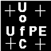
(b) $64\times 64$

(c) $512\times 512$

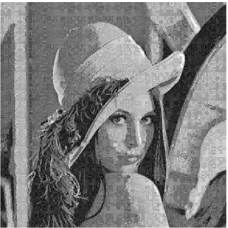
(d) $512\times 512$

Figure 1: Private Watermarking using the FFFT. (a) Original image, (b) watermark, (c) watermarked image in $\operatorname{GF}(13)$, (d) watermarked image in $\operatorname{GF}(73)$.

4 A Signature System

Apart from the private watermarking mode of operating, the described scheme can be interpreted from a different, new perspective. The present study proposes that the same system can be also considered as a method for signature data generation.

The watermark embedding process is now understood as a signature generation operation. The output signature $\mathbf{S}$ is simply defined as

$$\mathbf{S}\triangleq\mathbf{D}^{\prime},$$ (36)

where the image $\mathbf{D}^{\prime}$ is obtained according to Equation 32. Once obtained, the signature data can be made publicly available.

In this context, the original watermark extraction method becomes an authentication operation performed on raw data $\mathbf{D}$. The input data to be verified is $\mathbf{D}$, which is owned by the user. Therefore, the associated signature data, which can be retrieved from a trusted source, and the raw image can be submitted to the discussed method. An unaltered extracted watermark is an evidence of the integrity and authenticity of $\mathbf{D}$. In the case of a tampering attack, either on $\mathbf{D}$ or on $\mathbf{S}$, the extracted watermark can indicate the data corruption location.

It is worthwhile to emphasize that the aim is not to produce perceptually transparent watermarked images. Therefore, this approach completely diminishes the sensitivity to the value of the field characteristic, as experienced in the original methodology.

Again because the NTT transform domain lacks a physical meaning, even an alteration in the least significant bit of a signal can render a totally different NTT spectrum. This is a desirable property. No matter how subtle, tampering can produce strikingly noticeable differences in the recovered watermark. Consequently, this approach can verify the authenticity and integrity of raw digital data, providing means to spatially locate alteration regions.

5 Computational Results and Discussion

In this section, some computational experiments are performed to validate the proposed methods. Selected standard images available at the University of Southern California Signal and Image Processing Institute (USC-SIPI) Image Database [39] were submitted to the suggested watermarking scheme. Private watermarking and signature generation functionalities of the method were explored, with the application of the two-dimensional finite field cosine and Hartley transforms.

Generally the dimensions of a practical number theoretic transformation matrix $N\times N$ are smaller than usual image sizes. Typical values of the transform size $N$ are given in Table 1 and 2. Therefore, the required two-dimensional transforms are obtained conforming to a blockwise computation. This approach simply consists of decomposing a given host image into adjacent, equal sized, nonoverlapping blocks. These constituent blocks must match the dimensions of the considered two-dimensional transformation matrix. After that, each block is transformed and the resulting 2-D spectral blocks are reassembled, which results in a blockwise transformed image. Figure 2 illustrates the process. Accordingly, the discussed watermarking schemes are applied blockwise as well.

Figure 2: A blockwise two-dimensional transform application. The size of the the dashed blocks matches the two-dimensional transform blocksize $N\times N$.

Considering the FFCT, a raw image (Figure 3(a)) was processed and furnished the watermarked data displayed in Figure 3(c). Figure 3(d) shows the original image after the introduction of random artifacts on its pixel values. The modification consisted of incrementing the image pixels by one with probability $10^{-2}$. A wavy pattern was selected as the watermark (Figure 3(b)) and an FFCT over $\operatorname{GF}(7)$ with blocksize of two was chosen. Over $\operatorname{GF}(7)$, a possible choice is $\zeta=2+2j$, which induces an NTT of length equal to 2. This small blocksize was able to sharply indicate tampering locations (Figure 3(e)).

Similar results were obtained with the aid of the FFHT. Using an 8-point 2-D FFHT over $\operatorname{GF}(31)$ ($\zeta=4+4j$), a modification introduced into a raw image (Figure 4(a)) could be detected and assessed. Differently from the previous experiment, a smaller watermark was utilized (Figure 4(b)). After the calculations, the recovered watermark image (Figure 4(e)) clearly discloses the tampering and shows the interfered regions. Actually, the use of a small transform blocklength made possible to provide information on the nature of the modification. In this case, a small text had been written on the original image. If a larger transform were employed, this capability would be reduced, because the recovered watermark would present the tampered areas in larger blocks. Ultimately the accuracy of the tampering location would be mitigated.

Figures 5 and 6 illustrate the signature operation proposed in the current work. An original image (Figure 5(a)) was processed with the inclusion of a watermark (Figure 5(b)). Consequently, the signature image data depicted in Figure 5(c) was obtained. Being the calculations over $\operatorname{GF}(127)$, a visually low-quality image was attained. However, this is not important, because the Figure 5(c) is only intended to be used as signature data. Only its mathematical properties are relevant. A tampering consisting of incrementing a single pixel at position $(100,100)$ was applied to the original image, and Figure 5(d) was derived. The output of the authentication system is shown in Figure 5(e). As the chosen $\zeta$ for this calculations was $2+39j$, the transform blocksize was 32. Therefore, the precision of tampering positioning is restricted to $32\times 32$ pixel regions.

For an improved tampering location accuracy, one may consider shorter transforms, as in the experiment depicted in Figure 6. After signature generation in $\operatorname{GF}(251)$ using the FFHT with $\zeta=j$ (Figure 6(c)), the host data (Figure 6(a)) was maliciously tampered. Figure 6(d) shows that a forged image is introduced. This specific $\zeta$ implies a 4-point transform, which provides a potentially adequate tampering location accuracy. The recovered watermark clearly discriminates the modification site (Figure 6(e)).

Given a fixed subject image (Lena portrait), watermarked/signature images were generated via the method discussed herein, for all possible finite fields with characteristic ranging from 3 to 251. Both FFCT and FFHT were considered and $\zeta$ was chosen in such a way that 4-point 2-D transformations were guaranteed. Subsequently, the peak signal-to-noise ratio (PSNR) was adopted as a measure of the image deterioration after the watermarking process. For small values of $p$, visually imperceptible watermarks can be produced, since the resulting images present high PSNR values. However, for large values of $p$, the image quality becomes unacceptable for invisible watermarking purposes. Despite of that, for signature data generation, obtaining low PSNR values becomes less relevant. Quantitative data concerning the image degradation are summarized in Figure 7.

(a) $512\times 512$

(b) $512\times 512$

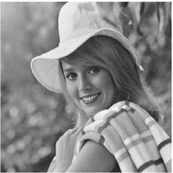
(c) $512\times 512$

(d) $512\times 512$

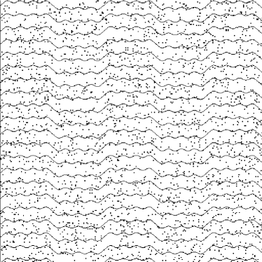
(e) $512\times 512$

Figure 3: Private watermarking using the FFCT. (a) Original image elaine.512.tiff (Elaine), (b) watermark (negative image for better visualization), (c) watermarked image, (d) tampered image with a Bernoulli distributed noise of $10^{-2}$ error probability, (e) extracted watermark with clear location of tampering (negative image for better visualization). Calculations were performed over $\operatorname{GF}(7)$ with $\zeta=2+2j$, transform size is 2.

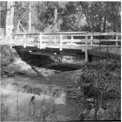
(a) $256\times 256$

(b) $64\times 64$

(c) $256\times 256$

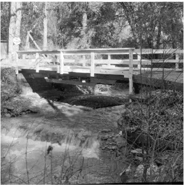
(d) $256\times 256$

(e) $256\times 256$

Figure 4: Private watermarking using the FFHT. (a) Original image 5210.tiff (Stream and bridge), (b) watermark, (c) watermarked image, (d) tampered image with the additive insertion of another image, (e) extracted watermark with a hidden message (send more money). Calculations were performed over $\operatorname{GF}(31)$ with $\zeta=4+4j$, transform size is 8.

(a) $256\times 256$

(b) $64\times 64$

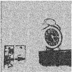
(c) $256\times 256$

(d) $256\times 256$

(e) $256\times 256$

Figure 5: Signature data generation using the FFCT. (a) Original image 5112.tiff (Clock), (b) watermark, (c) signature image (publicly available), (d) tampered image with the pixel at position $(100,100)$ incremented by one, (e) extracted watermark. Observe the fragility of the signature embedding: a single bit alteration made a whole block of recovered data to be distorted. Calculations were performed over $\operatorname{GF}(127)$ with $\zeta=2+39j$, transform size is 32.

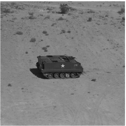
(a) $512\times 512$

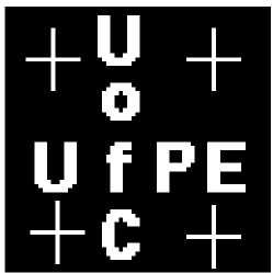
(b) $64\times 64$

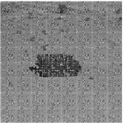
(c) $512\times 512$

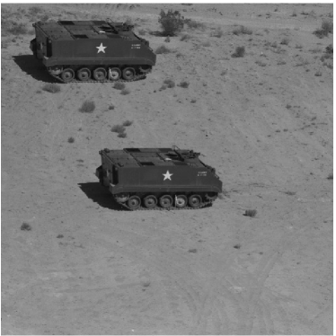
(d) $512\times 512$

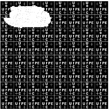
(e) $512\times 512$

Figure 6: Signature data generation using the FFHT. (a) Original image 7108.tiff (APC), (b) watermark, (c) signature image (publicly available), (d) tampered image, (e) extracted watermark. Calculations were performed over $\operatorname{GF}(251)$ with $\zeta=j$, transform size is 4.

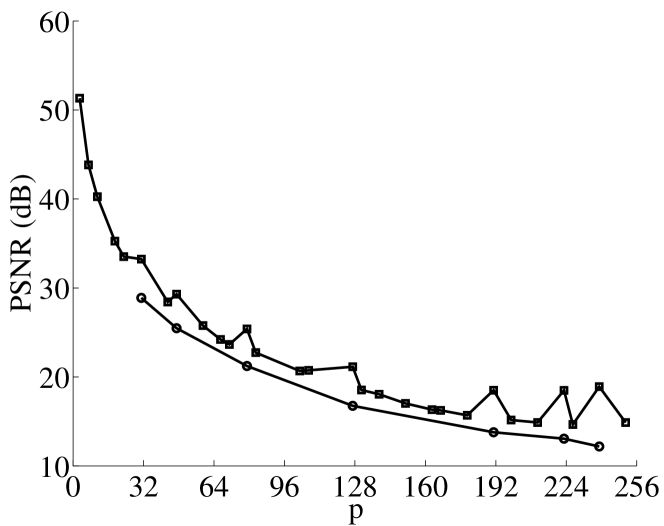
Figure 7: Quality degradation of watermarked images generated by the discussed method as a function of the finite field characteristic. The PSNR was employed to assess the image degradation. The Lena portrait was watermarked with 4-point 2-D FFCT (—$\circ$—) and FFHT (—$\Box$—) in all pertinent Galois fields $\operatorname{GF}(p)$, for $3\leq p\leq 251$.

6 Conclusion

The utilization of finite fields as an avenue for fragile watermarking was explored. The watermarking scheme suggested in [25] was amplified and generalized by the introduction of finite field trigonometrical transforms, such as the finite field cosine and Hartley transforms. The new proposed methodology generates signature data that can provide image authentication as well as tampering location capability.

References

- [1] J. J. Thomas, G. N. Larsen, and J. M. Keller, “Number theoretic transforms with independent length and moduli,” IEEE Transactions on Acoustics, Speech, and Signal Processing, vol. 31, no. 1, pp. 215–217, Feb. 1983.
- [2] R. M. Campello de Souza, H. M. de Oliveira, L. B. Espinola-Palma, and M. M. Campello de Souza, “Transformadas numéricas de Hartley,” in XVIII Simpósio Brasileiro de Telecomunicações (Brazilian Symposium on Telecommunications), Gramado, Brazil, Sep. 2000.
- [3] J. M. Pollard, “The fast Fourier transform over finite fields,” Mathematics of Computation, vol. 25, pp. 365–374, Apr. 1971.
- [4] V. S. Dimitrov, T. V. Cooklev, and B. Donevsky, “Generalized Fermat-Mersenne number theoretic transform,” IEEE Transactions on Circuits and Systems—II: Analog and Digital Signal Processing, vol. 41, no. 2, pp. 133–139, Feb. 1994.
- [5] ——, “Generalized Fermat transforms,” Advances in Computational Mathematics, vol. 41, pp. 27–41, 1992.
- [6] ——, “Number theoretic transforms over the golden section quadratic field,” IEEE Transactions on Signal Processing, vol. 43, no. 8, pp. 1790–1797, Aug. 1995.
- [7] J. Hong and M. Vetterli, “Hartley transforms over finite fields,” IEEE Transactions on Information Theory, vol. 39, no. 5, pp. 1628–1638, Sep. 1993.
- [8] S. Boussakta and A. G. J. Holt, “New number theoretic transform,” Electronics Letters, vol. 28, no. 18, pp. 1683–1684, Aug. 1992.
- [9] M. M. Campello de Souza, H. M. de Oliveira, R. M. Campello de Souza, and M. M. Vasconcelos, “The discrete cosine transform over prime finite fields,” Lecture Notes in Computer Science, vol. 3124, pp. 482–487, 2004.
- [10] R. M. Campello de Souza, H. M. de Oliveira, and A. N. Kauffman, “The Hartley transform in a finite field,” Journal of the Brazilian Telecommunications Society, vol. 14, no. 1, pp. 46–54, 1999.
- [11] R. M. Campello de Souza, H. M. de Oliveira, A. N. Kauffman, and A. J. A. Paschoal, “Trigonometry in finite fields and a new Hartley transform,” in 1998 IEEE International Symposium on Information Theory, Cambridge, MA, USA, Aug. 1998.
- [12] R. M. Campello de Souza, H. M. de Oliveira, L. B. Espinola-Palma, and M. M. Campello de Souza, “Hartley number theoretic transforms,” in IEEE International Symposium on Information Theory, Washington, D.C., USA, Jun. 2001.
- [13] D. Silva, R. M. Campello de Souza, and H. M. de Oliveira, “Transformadas em corpos finitos e grupos de inteiros gaussianos,” in XIX Simpósio Brasileiro de Telecomunicações (Brazilian Symposium on Telecommunications), Fortaleza, Brazil, Sep. 2001.
- [14] I. S. Reed and T. K. Truong, “The use of finite fields to compute convolutions,” IEEE Transactions on Information Theory, vol. 21, pp. 208–213, Mar. 1975.
- [15] R. C. Agarwal and C. S. Burrus, “Number theoretic transforms to implement fast digital convolution,” Proceedings of IEEE, vol. 63, pp. 550–560, Apr. 1975.
- [16] J. B. Martens, “Polynomial products by means of generalized number theoretic transforms,” IEEE Transactions on Acoustics, Speech, and Signal Processing, vol. 32, no. 3, pp. 668–670, Jun. 1984.
- [17] F. J. MacWilliams and N. J. A. Sloane, The Theory of Error Correcting Codes. North-Holland, 1988.
- [18] A. Schönhage and V. Stranssen, “Schnelle multiplikation großer zahlen,” Computing, vol. 7, pp. 281–292, 1971.
- [19] J.-J. Hsue and A. E. Yagle, “Fast algorithms for solving Toeplitz systems of equations using number-theoretic transforms,” Signal Processing, vol. 44, no. 1, pp. 89–101, Jun. 1995.
- [20] G. Madre, E. H. Baghious, S. Azou, and G. Burel, “Fast pitch modelling for CS-ACELP coder using Fermat number transforms,” in Proceedings of the 3rd IEEE International Symposium on Signal Processing and Information Technology, Dec. 2003, pp. 765–768.
- [21] A. E. Yagle, “Fast algorithms for matrix multiplication using pseudo-number theoretic transforms,” IEEE Transactions on Acoustics, Speech, and Signal Processing, vol. 43, no. 1, pp. 71–76, Jan. 1995.
- [22] G. A. Jullien and V. S. Dimitrov, “Two-dimensional transforms using number theoretic techniques,” in Computer Techniques and Algorithms in Digital Signal Processing, ser. Control and Dynamic Systems, C. T. Leondes, Ed. Academic Press, 1996, vol. 75, ch. 4, pp. 155–210.
- [23] T. Toivonen, J. Heikkilä, and O. Silvén, “A new algorithm for fast full search block motion estimation based on number theoretic transforms,” in Proceedings of the 9th International Workshop on Systems, Signals and Image Processing, P. Liatsis, Ed., Manchester, U.K., Nov. 2002, pp. 90–94.
- [24] T. Kriz and D. Bachman, “A number theoretic transform approach to image rotation in parallel array processors,” in IEEE International Conference on Acoustics, Speech, and Signal Processing, vol. 5, Apr. 1980, pp. 430–433.
- [25] H. Tamori, N. Aoki, and T. Yamamoto, “A fragile digital watermarking technique by number theoretic transform,” IEICE Trans. Fundamentals, vol. E85-A, no. 8, pp. 1902–1904, Aug. 2002.
- [26] E. T. Lin and E. J. Delp, “A review of fragile image watermarks,” in Proceedings of the Multimedia and Security Workshop (ACM Multimedia ’99) Multimedia Contents, Orlando, FL, USA, Oct. 1999, pp. 25–29.
- [27] M. George, J. V. Chouinard, and N. Georganas, “Digital watermarking of images and video using direct sequence spread spectrum techniques,” in Canadian Conference on Electrical and Computer Engineering, vol. 1, Edmonton, AB, Canada, May 1999, pp. 116–121.
- [28] C.-S. Li and H.-Y. M. Liao, “Multipurpose watermarking for image authentication and protection,” IEEE Transactions on Image Processing, vol. 10, no. 10, pp. 1579–1592, Oct. 2001.
- [29] C.-T. Li, “Digital fragile watermarking scheme for authentication of JPEG images,” IEE Proceedings - Vision, Image and Signal Processing, vol. 151, no. 6, pp. 460–466, Dec. 2004.
- [30] H. Lu, R. Shen, and F.-L. Chung, “Fragile watermarking scheme for image authentication,” Electronics Letters, vol. 39, no. 12, pp. 898–900, Jun. 2003.
- [31] M. Chen, Y. He, and R. L. Lagendijk, “A fragile watermark error detection scheme for wireless video communications,” IEEE Transactions on Multimedia, vol. 7, no. 2, pp. 201–211, Apr. 2005.
- [32] J. Hu, J. Huang, D. Huang, and Y. Q. Shi, “Image fragile watermarking based on fusion of multi-resolution tamper detection,” Electronics Letters, vol. 38, no. 24, pp. 1512–1513, Nov. 2002.
- [33] D. Kundur and D. Hatzinakos, “Digital watermarking for telltale tamper proofing and authentication,” IEE Proceedings - Vision, Image and Signal Processing, vol. 87, no. 7, pp. 1167–1180, Jul. 1999.
- [34] P. Campisi, M. Carli, G. Giunta, and A. Neri, “Blind quality assessment system for multimedia communications using tracing watermarking,” IEEE Transactions on Signal Processing, vol. 51, no. 4, pp. 996–1002, Apr. 2003.
- [35] D. Zheng, J. Zhao, W. J. Tam, and F. Speranza, “Image quality measurement by using digital watermarking,” in Proceedings of the 2nd IEEE Internatioal Workshop on Haptic, Audio and Visual Environments and Their Applications, Sep. 2003, pp. 65–70.
- [36] G. H. Hardy and E. M. Wright, An Introduction to the Theory of Numbers. Oxford University Press, 1945.
- [37] R. N. Bracewell, The Hartley Transform. Oxford University Press, 1986.
- [38] R. E. Blahut, “Transform techniques for error control codes,” IBM Journal of Research and Development, vol. 23, no. 3, pp. 299–315, May 1979.
- [39] Signal and Image Processing Institute, “The USC-SIPI image database,” ¡http://sipi.usc.edu/services/database/Database.html¿, 2005, University of Southern California.