On fibrils and field lines: The nature of H$\alpha$ fibrils in the solar chromosphere

Abstract

Observations of the solar chromosphere in the line-core of the H$\alpha$ line show dark elongated structures called fibrils that show swaying motion. We performed a 3D radiation-MHD simulation of a network region, and computed synthetic H$\alpha$ images from this simulation to investigate the relation between fibrils and the magnetic field lines in the chromosphere. The synthetic imagery shows fibrils just as in observations. The periods, amplitudes and phase-speeds of the synthetic fibrils are consistent with those observed. We analyse the relation between the synthetic fibrils and the field lines threading through them, and find that some fibrils trace out the same field line along the fibril’s length, but there are also fibrils that sample different field lines at different locations along their length. Fibrils sample the same field lines on a time scale of $\sim 200$ s. This is shorter than their own lifetime, and thus they do not sample the same field lines during their entire life. We analysed the evolution of the atmosphere along a number of field lines that thread through fibrils and find that they carry slow-mode waves that load mass into the field line, as well as transverse waves that propagate with the Alfvén speed. Transverse waves propagating in opposite directions cause an interference pattern with complex apparent phase speeds. These wave motions are present on top of a slow drift of the field line through the computational domain.

The relationship between fibrils and field lines is complex. It is governed by constant migration and swaying of the field lines, their mass loading by slow modes and subsequent draining, and their actual visibility in H$\alpha$. Field lines are visible where they lie close to the optical depth unity surface. The location of the latter is governed by the height at which the column mass in the chromosphere reaches a certain value. The visibility of field line at a fixed time is thus not only governed by its own mass density but also by the mass density of the material above it. We conclude that using the swaying motion of fibrils as a tracer of chromospheric transverse oscillations must be done with caution.

1. Introduction

Images of the solar disk taken in the line core of the H$\alpha$ line display dramatic elongated dark and bright features called fibrils and mottles. They are present everywhere, except in the quietest Sun away from concentrations of magnetic field. Their elongated shape and presence wherever the magnetic field is strong, suggest that fibrils and mottles outline the plane-of-the-sky component of the magnetic field.

There is, however, very little direct observational evidence for this suggestion in network areas and quiet Sun regions. The H$\alpha$ line itself is ill-suited for measuring chromospheric magnetic fields (Socas-Navarro & Uitenbroek, 2004). The plane-of-the sky magnetic field around sunspots was measured by de la Cruz Rodríguez & Socas-Navarro (2011) using spectropolarimetry in the Ca II 854.2 nm line. This line has a similar formation height as H$\alpha$ (Leenaarts et al., 2013b) and shows similar fibril structure. Their conclusion is that most of the time, but not always, fibrils appear to be aligned with the plane-of-the sky magnetic field. To our knowledge no studies in quiet Sun have been done so far.

On the modelling side only Leenaarts et al. (2012) have reproduced fibril-like structures in synthetic H$\alpha$ images computed from a snapshot of a radiation-MHD (RMHD) simulation of the solar atmosphere. They found that the fibril-like structures in the simulation indeed trace out the horizontal component of the magnetic field, but did not measure the alignment of the 3D magnetic field vector and the fibril-like structure. It is thus not clear whether fibrils trace out single field lines, or that they actually intersect a set of different field lines that happen to have a horizontal component parallel to the fibril.

For a subset of dark elongated H$\alpha$ features, there is compelling evidence based on their dynamical behaviour that they align with the magnetic field in all three dimensions: The tops of so-called ’dynamic fibrils’ in active regions and mottles in quiet Sun show parabolic trajectories as function of time. RMHD models show that they can be explained as slow-mode acoustic shocks that propagate only along the direction of the magnetic field (Hansteen et al., 2006; De Pontieu et al., 2007; Rouppe van der Voort et al., 2007; Rouppe van der Voort & de la Cruz Rodríguez, 2013). Another class of fibrils is present in network areas and active regions. They appear as dense rows of elongated dark features that span the chromosphere between areas with opposite magnetic polarity in the photosphere. The horizontal size of these fibrils ($\sim 30$ Mm) is much larger than the extent of the optically thick H$\alpha$ core emission above the solar continuum limb ($<\sim$5 Mm, see, e.g, Simon & White, 1966), and estimates of the typical H$\alpha$ formation height of 0.5 Mm to 3 Mm (Vernazza et al., 1981; Leenaarts et al., 2012) Therefore, in a simplified view where we assume magnetic field lines to be semi-circular, we do not expect these fibrils to trace the magnetic field in 3D, because the loop height is much larger than the H$\alpha$ formation height. While field lines in reality will not be semi-circular, the relation between fibrils and field lines remains unclear.

Understanding this relationship is relevant because H$\alpha$ is one of the most-used diagnostics of the chromosphere, so improving our knowledge of its line formation will help understanding the physics of the chromosphere. In addition, H$\alpha$ is used as a constraint on magnetic field extrapolations (e.g., Wiegelmann et al., 2008; Jing et al., 2011), which requires understanding the fibril-field line relation. Finally, transverse oscillations in fibrils are used in chromospheric seismology.

Chromospheric seismology aims to derive properties of the chromosphere through measuring properties of observed oscillations and interpreting them as a certain types of waves. Oscillations of fibrils seen in the H$\alpha$ line core have been interpreted as kink waves: transverse incompressible oscillations of a tube of high mass density that is aligned with the magnetic field and is embedded in a medium with lower mass density. In this view, measurement of the periods $P$, wave displacement amplitudes $A$ and phase speeds of perturbation of the H$\alpha$ fibrils, and possibly their variation along the length of individual fibrils, then allows derivation of chromospheric properties. The period and displacement can be converted to velocity amplitudes $V$ if one assumes sinusoidal motion. The velocity amplitude together with an assumed mass density allows computation of the energy density of the wave. If phase speeds are measured then one can also derive the strength of the magnetic field and the energy flux carried by the wave.

In an observation of quiet Sun including some network boundary Kuridze et al. (2012) measured lifetimes of 42 mottles/fibrils and the period and amplitude of their transverse oscillations in a time-series of H$\alpha$ line-center images. Morton et al. (2013) analyzed the same dataset in more detail and derived improved statistics on the period and displacement of transverse fibril oscillations, finding an average period of 94 s and an average displacement of 71 km.

Kuridze et al. (2013) looked at a different quiet Sun dataset and presented three fibrils for which apparent phase speeds were measured. They found evidence of apparent phase speeds increasing from 40 km s^-1 to 120 km s^-1 along one fibril, and a fibril with signal of opposite phase speeds of +101 km s^-1 and -79 km s^-1 respectively, suggestive of two waves traveling in opposite direction. They also reported on a fibril oscillation with an apparent phase speed of 350 km s^-1, which they interpret as a standing wave pattern caused by oppositely directed waves.

In a recent paper, Morton et al. (2014) derived a velocity power spectrum of transverse H$\alpha$ oscillations in a quiet-Sun region and an active region and compared the power spectrum with the coronal transverse motion power spectrum derived from observations with the Coronal Multi-channel Polarimeter instrument

(Tomczyk & McIntosh, 2009), to estimate the frequency-dependent damping of transverse waves between the chromosphere and corona.

The above discussion shows that H$\alpha$ fibril seismology has the potential to be a powerful tool for diagnosis of chromospheric physical properties and the transport of energy by transverse oscillations from the photosphere into the outer solar atmosphere. However, the validity of this approach depends critically on two related assumptions:

1. fibrils trace single magnetic field lines at any given instant in time;

2. fibrils trace the same field line during their lifetime.

The fibrils most likely do trace out the horizontal component of the magnetic field, but as we have argued, it is not known whether fibrils also follow the vertical component of the field.

For the second assumption there is no observational evidence. We argue that it not at all clear that this is the case: Leenaarts et al. (2012) show that low H$\alpha$ line-core intensity typically corresponds to a large formation height, and that the line opacity is proportional to the mass density. Their simulation shows that fibrils correspond to mountain-ridge like structures of increased mass density. Dark fibrils are thus most likely structures that are over-dense in the horizontal direction compared to their surroundings. Even if a fibril traces out a single field line at a given instant in time, it is thinkable that this field line is drained of its mass while a neighbouring field line gets filled with mass. The H$\alpha$ fibril will then appear to move, while the actual field lines do not.

The main aim of this paper is to investigate the relation between magnetic field lines in a RMHD simulation of the solar atmosphere and the fibril-like structures (from now on we call them just fibrils) in a time series of synthetic H$\alpha$ images computed from the simulation. We use the results of the investigation to see to what extent the assumptions made in chromospheric seismology are valid, by analysing the time evolution of the fibrils and magnetic field lines that thread through them. Finally we analyse the evolution of the atmosphere along those fibril-threading field lines to investigate the dynamics of the simulated chromosphere.

In Section 2 we describe the radiation-MHD simulation and the subsequent radiative transfer modelling. Section 3 describes the observations that we use. In Section 4 we treat the fibrils in the synthetic images as observations to establish that they show the same oscillatory behaviour as the observations. Section 5 describes the reduction of the RMHD simulation data to extract properties along selected magnetic field lines and in Section 6 we analyse the relation between the fibrils and the magnetic field lines. We finish with a discussion and our conclusions in Section 7.

2. Simulations and radiative transfer

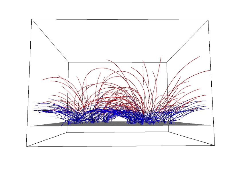
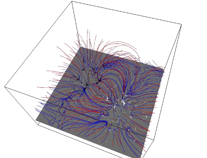
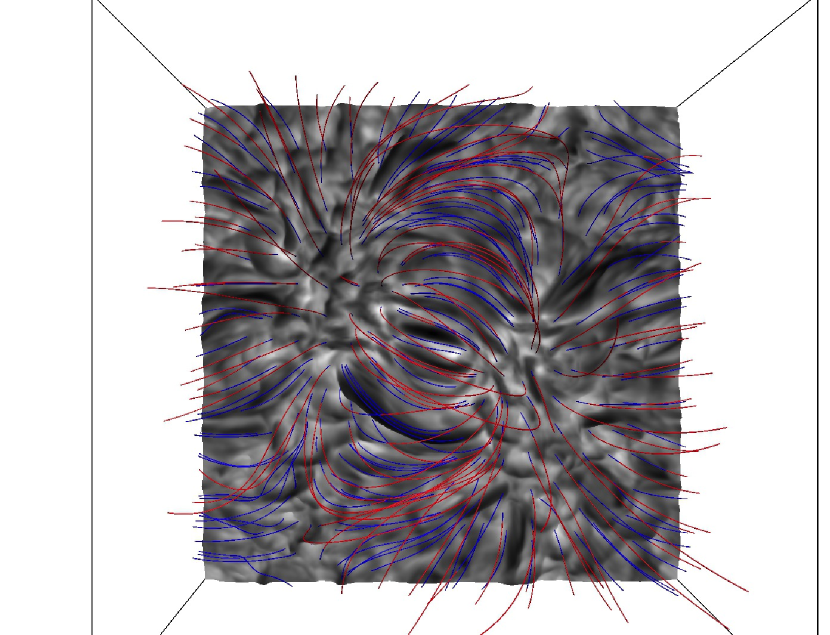
Figure 1.— Magnetic field configuration in the RMHD simulation. The wire frame outlines the border of the computational domain. Each panel shows the same set of magnetic field lines, color coded with the local temperature, blue for $T<20$ kK, red for $T\geq 20$ kK. Top and middle panel: side and top view of the domain. The gray-scaled plane displays the vertical magnetic field at z=0 Mm. Bottom panel: The gray-scaled surface is the H$\alpha$ line-core height of optical depth unity, color coded with the corresponding H$\alpha$ vertically emergent intensity. Only the section of the field lines above the surface of optical depth unity is displayed. The visualization was created with VAPOR (Clyne et al., 2007).

We performed a 3D radiation-MHD simulation of a part the solar atmosphere using the Bifrost code (Gudiksen et al., 2011). This code solves the equations of resistive MHD on a staggered Cartesian mesh. In addition to the MHD equations the simulation included optically thick non-LTE radiative transfer in the photosphere and low chromosphere, parameterized radiative losses and gains in the upper chromosphere, transition region and corona, thermal conduction along field lines and an equation of state that takes the non-equilibrium ionization of hydrogen into account.

The simulation was run on a grid of $504\times 504\times 496$ grid cells, with an extent of $24\times 24\times 16.8$ Mm. In the vertical direction the grid extends from 2.4 Mm below to 14.4 Mm above average optical depth unity at 500 nm, encompassing the upper convection zone, photosphere, chromosphere and lower corona. The $x$ and $y$-axes are equidistant with a grid spacing of 48 km. The $z$-axis is non-equidistant. It has a grid spacing of 19 km between $z=-1$ and $z=5$ Mm, while the spacing increases towards the upper and lower boundaries to a maximum of 98 km at the coronal boundary. The simulation has periodic boundary conditions in the two horizontal directions and open upper and lower boundaries.

The magnetic field configuration is mainly bipolar, chosen such that it leads to a small network-like configuration. It was created by specifying the magnetic field at the bottom boundary and using a potential field extrapolation to compute the field throughout the computational domain. The magnetic field was inserted into a relaxed hydrodynamical simulation and was then allowed to evolve freely. The simulation was subsequently run for 3000 s of solar time using LTE ionization, and then the non-equilibrium hydrogen ionization was switched on. Afterwards the simulation was run for 2240 s of solar time. We use a dataset of 1200 s of solar time (121 snapshots taken at 10 s intervals) starting 830 s after non-equilibrium ionization was switched on. The first snapshot of our time series is the same as was used in Leenaarts et al. (2012); Štěpán et al. (2012); Leenaarts et al. (2013a, b) and Pereira et al. (2013). The snapshots are publicly available for download. The whole simulation is described in more detail in Carlsson et al. (2015).

The synthetic H$\alpha$ imagery was computed following Leenaarts et al. (2012). In short, we use the radiative transfer code Multi3d (Leenaarts & Carlsson, 2009) to solve the non-LTE radiative transfer problem in 3D geometry for a 5-level-plus-continuum hydrogen atom. Owing to the strong scattering in the Lyman and Balmer lines it is essential to include 3D effects. The Lyman-$\alpha$ and Lyman-$\beta$ lines are treated with Doppler absorption profiles only to approximate PRD effects. In order to save computation time we down-sampled the Bifrost snapshots to half resolution in the horizontal direction, and solved the radiative transfer only every second snapshot, i.e, 61 snapshots at 20 s cadence with a grid size of $252\times 252\times 496$ cells. This is a slight improvement over Leenaarts et al. (2012), where the atmosphere was also down-sampled in the vertical direction. We performed a test computation at the full resolution of the RMHD simulation, and found that the down-sampling reduces image sharpness but otherwise does not affect our results.

In Figure 1 we show a characterisation of the magnetic field in the simulation at $t=600$ s in our time series. The magnetic field exhibits a large-scale bipolar structure in the photosphere; as a consequence the chromosphere and corona are pervaded by loop-like structures. The majority of the magnetic field closes in the chromosphere: the average unsigned field at $z=0$ is 29.3 G, at z=0.8 Mm it reaches only 50% of this value and at z=3.3 Mm 25%. The bottom panel of Figure 1 shows an iso-surface of the H$\alpha$ line-core height of optical depth unity, colored with the corresponding H$\alpha$ intensity, illustrating that the fibrils roughly align with the horizontal component of the magnetic field.

3. Observations

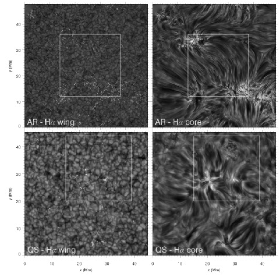
Figure 2.— Example H$\alpha$ images of the active region dataset taken on June 15, 2008 (top) and the quiet Sun dataset taken on May 5, 2011 (bottom). The left-hand column shows images in the red wing of the line, the right-hand column the profile-minimum intensity. The subregions used in Figure 4 are indicated by white boxes.

In Section 4 we compare the synthetic H$\alpha$ imagery with observations. These observations were obtained with the CRisp Imaging SpectroPolarimeter (CRISP, Scharmer et al., 2008) at the Swedish 1-m Solar Telescope (SST, Scharmer et al., 2003a) on La Palma.

We use a dataset of the remains of active region AR10998 taken on June 15, 2008 at 7:53 UT, with a duration of 27 minutes at 6.8 s cadence. The data were taken close to disk-center, at $\mu=0.98$. The H$\alpha$ line was sampled at 25 positions, equidistant with 0.1 Å steps between $-1.6$ Å and $+0.8$ Å from line center. We refer to this dataset as Active Region (AR).

A second dataset was acquired on May 5, 2011 at 7:38 UT. The H$\alpha$ spectral line was sampled with 35 line positions, from $-$2.064 Å to $+$1.290 Å, and equidistant 86 mÅ stepping between $\pm$1.290 Å. The time to complete a full line scan was 8 s. The target area was a quiet 60$\times$60″region at $\mu=1.0$. We refer to this dataset as Quiet Sun (QS).

Both datasets were captured during excellent seeing conditions, and the image quality was improved by the adaptive optics system of the SST (Scharmer et al., 2003b) and post-processing using Multi-Object Multi-Frame Blind Deconvolution (MOMFBD, van Noort et al., 2005) image restoration. For the data reduction we followed early versions of parts of the CRISPRED data processing pipeline (de la Cruz Rodríguez et al., 2014). Figure 2 shows example images of the AR and QS datasets.

4. Comparison of observed and simulated H$\alpha$ fibrils

4.1. H$\alpha$ as velocity diagnostic of fibrils

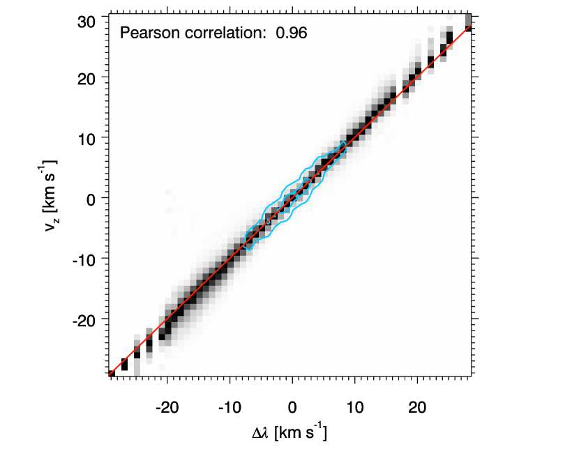
Figure 3.— Scaled joint probability density functions of the Doppler shift of the H$\alpha$ profile minimum (positive is redshift) and the vertical velocity at optical depth unity at that Doppler shift (positive is down flow). Each column in the panels is scaled to maximum contrast to increase visibility. The inner blue contour includes 50% of all pixels, the outer contour 90%. The red line denotes the line $v_{z}=\Delta\lambda$.

Our SST observations include a sampling of the line profile and we can thus use them to compare Doppler-shifts in the observed and simulated datasets. Because fibrils are most clearly visible in line-core images, we use the Doppler-shift of the profile minimum as their velocity diagnostic.

Leenaarts et al. (2013b) showed that the Dopplershift of the central line-profile minima of the Mg II h&k lines exhibit remarkable correlation with the vertical velocity at the height of optical depth unity. They are thus excellent velocity diagnostics. The high correlation for the Mg II lines is caused by the small ($\simeq 2.5$ km s^-1) Doppler width of the absorption profile and the steep increase of optical depth with geometric depth causing only a small height range to be sampled. The H$\alpha$ line has five times larger Doppler width. Numerical simulations indicate that its contribution function to intensity is often non-zero over a height range of 1 Mm or more (Leenaarts et al., 2012). We thus expect H$\alpha$ to perform somewhat worse as a velocity diagnostic than Mg II h&k.

We computed the correlation between the Doppler shift of the line-profile minimum and the vertical velocity at optical depth unity at the wavelength of the profile minimum based on all pixels in our synthetic time-series.

The results are displayed in Figure 3. The correlation is indeed not as good as for Mg II h&k, but its Pearson correlation coefficient is still very high at 0.96. We conclude therefore that the H$\alpha$ line is a good velocity diagnostic for those layers that are sampled by the profile minimum. Test with the observational datasets show that traditional Dopplergrams created by subtracting and normalizing intensity images at equal wavelength separation from line center are visually very similar to the Doppler-shift of the profile minimum. The advantages of using profile-minimum Dopplershift maps is that it provides the vertical velocity in absolute units, and that the profile-minimum intensity provides a direct visualization of the structures – fibrils in this paper – for which the velocity is measured.

4.2. Comparison of the appearance of synthetic and observed H$\alpha$ fibrils

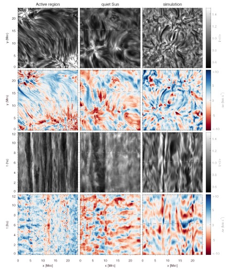
Figure 4.— Comparison of images and space-time diagrams of fibrils in an active region (left), quiet Sun (middle) and the simulation (right). Rows, from top to bottom display H$\alpha$ profile-minimum intensity images, H$\alpha$ line-core Doppler-shift images, intensity space-time diagrams, and Doppler-shift space-time diagrams. The dashed lines specify the location of the space-time cut in the images and vice versa. Blue color in the Doppler-shift panels corresponds to upflow. Time is given in units of hecto-seconds ($10^{2}$s ) in this and all following figures.

The RMHD simulation incorporates many of the physical processes that act in the solar chromosphere and indeed shows fibrilar structure reminiscent of observations. However, the separation of the opposite polarity patches in the photosphere is only $\sim 10$ Mm, considerably smaller than the typical size of a supergranule ($\sim 30$ Mm, e.g. Simon & Leighton, 1964), and the maximum length of the simulated fibrils is thus shorter than possible on the sun. The finite resolution of the simulation (48 km horizontal, 19 km vertical) does not allow horizontal structures smaller than $\sim 100$ km to form. It is therefore worthwhile to analyze in more detail how the simulated fibrils appear and behave in comparison with observed ones.

In Figure 4 we compare fibrils in the AR and QS observations and the simulation. The panels showing the observations display the same spatial and temporal extent as the simulation to allow for fair comparison.

The AR area has a cluster of photospheric magnetic elements in the upper-left and lower-right corners of the field-of-view (FOV). Between these elements a carpet of long and finely structured fibrils is present. The QS image displays a few broad and short dark fibrils (also called mottles, see Tsiropoula et al., 2012, and references therein) that extend towards to top of the image. The corresponding H$\alpha$ wing image shows a small group of photospheric magnetic elements in the lower part of the image (see Figure 2).

The simulated fibrils appear as a cross between the AR and QS ones, they typically are not as wide as in the QS, but also not as long, slender and densely packed as in the AR area. The simulated intensity contrast is similar to the observed one.

The second row shows images of the Dopper-shift of the line core. The overall structuring is similar to the intensity images. Both the AR and QS images show upward and downward moving fibrils, but the AR panel shows Dopper-shift variation perpendicular to the magnetic field on smaller spatial scales.

The two bottom rows compare time-distance diagrams of the line-core intensity and Doppler-shift. The line-core panels (third row) show the characteristic swaying motions of the fibrils. The swaying fibril tracks are ubiquitously present in all three datasets. The AR dataset typically shows tracks that remain visible during a longer time than in the QS panel, and the simulation again shows characteristics somewhere in between the AR and QS data.

In the bottom row we show the time evolution of the profile-minimum Doppler shift along the same cut across the fibrils. All three panels show elongated structure only at the location of the very darkest fibrils. The rest of the panel is dominated by oscillations with periods of 3 to 5 min and a coherency length along the slit of $\sim 4$ Mm in the AR and $\sim 10$ Mm in the QS observations. These coherent oscillations are most likely the result of buffeting from below by internetwork acoustic shocks excited by $p$-modes and granular buffeting (Rutten et al., 2008). The simulation displays an oscillation with a typical period of 4 min that is coherent along the whole 24 Mm cut. This is the signature of shocks driven by global radial box oscillations – the simulation counterpart of $p$-modes – excited by the convection (Stein & Nordlund, 2001).

The AR panel shows smaller Doppler-shift amplitude ($\pm 7$ km s^-1, RMS of 1.7 km s^-1) than the QS (amplitude -8 to +14 km s^-1, RMS of 2.5 km s^-1) and simulated (amplitude -12 to +11 km s^-1, RMS of 2.9 km s^-1) data.

It is unclear what is causing the difference in pattern between the intensity and Doppler shift time-distance diagrams. It is possible that many of the fibrils have an optical thickness of close to unity, so that the Doppler-shift of the profile minimum is partially determined by the sub-canopy domain, which is full of acoustic waves and shocks. Another possibility is that we see the actual upward and downward motion of the fibrils themselves, and that this is residual motion caused by the reflection of sub-canopy waves at the $\beta=1$ surface, as demonstrated in the simulations of Rosenthal et al. (2002). The reflection of the acoustic waves can have a significant signal into layers where $\beta<0.1$, where fibrils are presumably located. This scenario is supported by the fact that the Doppler-shift amplitude in the AR dataset, where H$\alpha$ forms much higher above the $\beta=1$ surface, are smaller than in the QS, where H$\alpha$ samples closer to the $\beta=1$ surface. Of course another mechanism altogether remains possible too.

Focusing back on our present purpose: we have established that the simulation qualitatively reproduces many of the features of the appearance of fibrils in network and quiet Sun, in both intensity and Doppler shift. The fibril density and width in the simulations are intermediate between AR and QS, the simulated Dopplershifts are closer to the QS properties than to the properties of the AR.

4.3. Transverse oscillations of synthetic fibrils

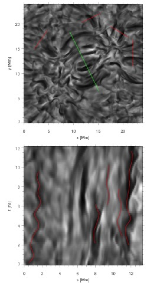
Figure 5.— Top panel: synthetic H$\alpha$ line-core image at t=600 s. The location of the time-distance diagrams used to measure fibril oscillation motions are overplotted. Bottom panel: time-distance diagram along the green cut in the upper panel, with fibril tracks overplotted in red.

Figure 6.— Histogram of the properties of the oscillations of the simulated fibrils. Left: maximum transverse displacement; middle: period; right: maximum transverse velocity.

We now turn our attention to the periods, displacement and velocity amplitudes of the synthetic fibrils. After manual inspection of the data we placed five cuts through the data that showed clear oscillations of dark fibrils (see Figure 5). There are many more fibrils that appear to sway when playing the image sequence as a movie, but whose time-distance diagram does not show an unambiguous swaying track. After selecting the cuts with clear swaying we manually traced the swaying fibril tracks. We also examined automated detection algorithms after unsharp masking of the data to bring out contrast, but found that this leads to many false detections. These are in particular connected with the bright-dark pattern of the box oscillations, that after unsharp masking often give rise to sinusoidal tracks that are not associated with dark fibrils.

In the cuts we found 13 fibrils that could be unambiguously followed for one period or more. Because we found that the fibrils show oscillatory behavior, but rarely with constant amplitude and period, we also measured periods and amplitudes by hand. For each space-time track we removed a linear trend. Then we measured the space and time coordinate of each extremum ($t_{i},x_{i}$). The time difference between two consecutive maxima or minima gives one measurement of a period $P$: $P_{i}=t_{i+1}-t_{i-1}$. The spatial difference between two consecutive extrema yields a measurement of the transverse displacement $d$: $d_{i}=0.5(x_{i+1}-x_{i})$. Finally we computed the velocity amplitude $v$ as $v_{i}=\pi(d_{i-1}+d_{i})/P_{i}$. In total we measured 40 displacements, 31 periods and 31 velocity amplitudes.

The results of our measurements are shown in Figure 6. The average (standard deviation) of the displacement is 158 km (98 km), for the period it is 221 s (70 s) and for the velocity amplitude it is 4.5 km s^-1 (1.8 km s^-1). Morton et al. (2013) measure smaller average displacements and periods, 71 km and 94 s. We believe this to be at least partially caused by an event selection bias caused by the higher spatial and temporal resolution of their observations and their automated versus our manual event selection. The observations used by Morton et al. have a spatial pixel size of 50 km and a temporal resolution of 7.7 s, compared to 96 km and 20 s for the simulations. The observations thus in principle allow detection of oscillations at half the amplitude and 2.6 times smaller period. The automated detection algorithm used by Morton et al. (2013) also picks up weak signals, while we focus on the oscillations of the most prominent dark fibrils. Another possible source of the difference is the resolution of the simulation, that might not support oscillations below a certain displacement amplitude.

The average velocity amplitude that we find is the same as Morton et al. (2013), but the synthetic distribution lacks the tail of high amplitude events detected in the observations.

In summary, we find that the swaying fibrils in the synthetic H$\alpha$ imagery have periods, maximum displacements and velocity amplitudes that are consistent with those observed. The lack of short-period and low-displacement events are possibly caused by finite spatial resolution of the simulation, the spatial resolution and cadence of the synthetic images and a selection bias.

4.4. Phase speeds

Table 1Approximate phase speeds in synthetic fibrils (km s^-1)

54	18	49
33	60	56
320	27	16

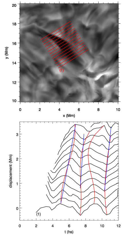
Figure 7.— Phase speeds in a simulated fibril. Top panel: H$\alpha$ image of the dark fibril at $t=600$ s, with the cross-cuts used in the bottom panel overplotted in red. Bottom panel: The black curves show the displacement of the fibril along each of the cross cuts in the top panel as function of time, with a linear trend removed. The track labelled (1) corresponds to the cut with the same label in the upper panel. The other tracks have been shifted vertically by the distance between the corresponding cross-cut and the cut labeled (1) in the upper panel. Blue lines: linear fits to selected extrema. Red curves: third-order polynomial fits to the strongest extrema.

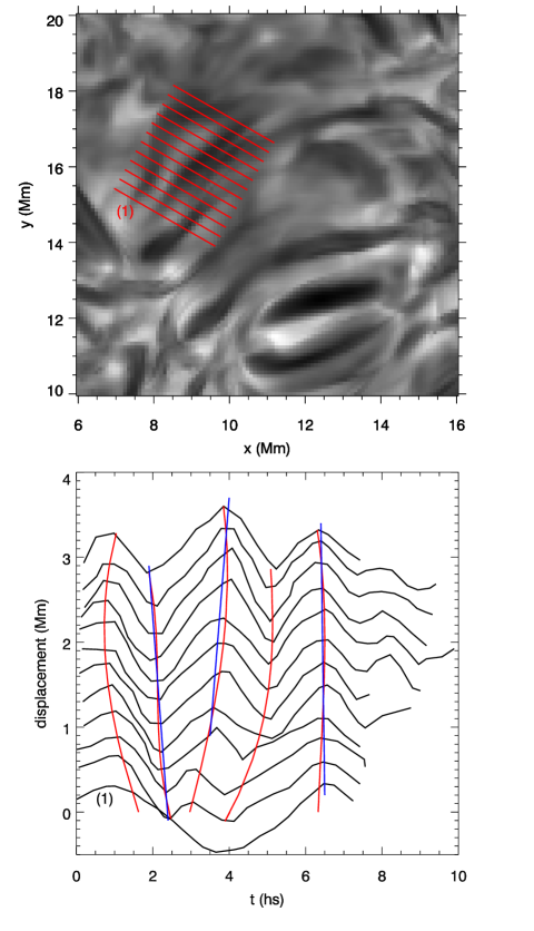
Figure 8.— Same as Figure 7, but for a another fibril.

In our synthetic H$\alpha$ time series we found a few instances of strong fibrils for which it was possible to measure phase speeds. We placed a number of cross-cuts intersecting the fibrils at different places along their length and measured the $st$-track along each cut. We then subtracted a linear fit from the tracks to remove systematic drift. In Figures 7 and 8 we show two strong, long-lived fibrils and their swaying along the cross-cuts. The phase speeds of the extrema are typically not constant, but show acceleration, deceleration and sometimes even a reversal of direction. The fibril in Figures 8 shows clear indication of a minimum traveling in one direction along the fibril, and the following maximum in the other direction. The complexity of these phase diagrams is suggestive of an interference pattern caused by waves traveling in opposite directions. For those instances where the phase speed was nearly constant over most of the length of the fibrils we show the measured speeds in Table 1, they range from 16 km s^-1 to 320 km s^-1. This is consistent with Kuridze et al. (2013), who report phase speeds of 79 km s^-1, 101 km s^-1 and 360 km s^-1.

We conclude that the simulation reproduces the observed properties sufficiently well to assume that the simulation contains the essential physics driving transverse oscillations of fibrils. In Section 5 we take a closer look at the MHD structures and their dynamics that give rise to the synthetic H$\alpha$ fibrils.

5. Reduction of the RMHD data

We chose to reduce the data using a magnetic field line based approach. The rationale for this approach is that fibrils form in the chromosphere in a low plasma $\beta$ environment. Both slow waves and Alvén waves therefore propagate parallel to the field lines, and analysis of the data along field lines then provides a natural way to bring out those waves.

We planted 80 seed points in the simulation at $t=600$ s along a number of fibrils in the corresponding H$\alpha$ image. The $x$ and $y$ coordinates of the seed points thus follow the fibrils, and are spaced about 0.5 Mm apart. As $z$-coordinate of the points we chose the height of optical depth unity for the profile minimum. From each seed point we traced a magnetic field line. In order to trace the same field line over time we advected the field line apex both forward and backward in time, used the new location to trace a new field line and repeated this until we obtained the time evolution of the entire field line. In Figure 9 we show the location of the seed points and the field lines traced from them.

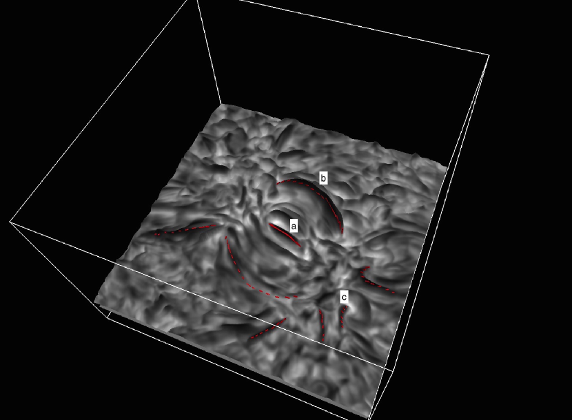
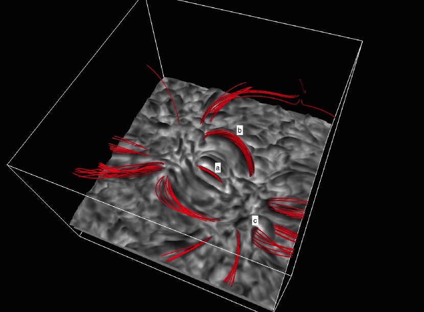
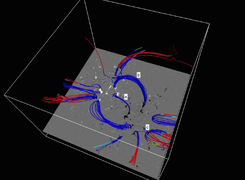
Figure 9.— Three-dimensional visualisation of selected field lines that thread through H$\alpha$ fibrils at $t=600$ s in the simulation. Top: Surface of optical depth unity, colour coded with the emergent H$\alpha$ intensity, with red line segments indicating the field line seed points and the local direction of the magnetic field. Middle: Same as top panel, but now showing the part of the field lines that extends above the optical depth unity surface. Bottom: The same field lines, but now shown on top of the vertical magnetic field at $z=0$ Mm. The field lines are colour coded with temperature: dark blue for $T<17$ kK; red for $T>100$ kK; other colours indicate intermediate values. The labels a, b and c indicate fibrils and associated flux bundles shown in Figure 11.

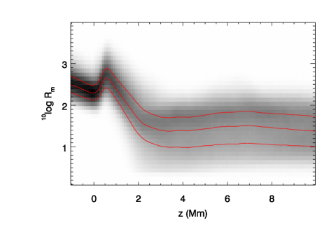
Figure 10.— Distribution of the magnetic Reynolds number as function of height at t=600 s in the Bifrost simulation.The red curves indicate the 25th, 50th and 75th percentile.

The validity of this approach is limited by the finite time resolution of our snapshot series (10 s cadence), which limits the ability to accurately follow test particles in time, and the magnetic Reynolds number $R_{\mathrm{m}}$, which determines how well the assumption of frozen-in magnetic flux holds. Bifrost employs a space and time variable, non-isotropic magnetic diffusion coefficient $\boldsymbol{\eta}(\boldsymbol{r},t)$, so we cannot give a single value for $R_{\mathrm{m}}=(LU)/\eta$. Instead we show the joint probability density distribution in Figure 10, assuming a typical length scale $L$ of 1 Mm and a typical velocity $U$ of 10 km s^-1. The Reynolds number is always larger than unity. Even at heights where it is smallest, 75% of the grid cells has $R_{\mathrm{m}}>10$ and 50% has $R_{\mathrm{m}}>30$. The frozen-in condition thus holds for a large fraction of the domain, but we also expect locations where diffusion is important. In Section 6 we show that many field lines that we analyse remain anchored in the same photospheric field concentrations for the 1200 s duration that we consider, and evolve smoothly in time, indicating sufficient time resolution and validity of the frozen-in assumption.

However, there are also instances where the field lines evolve in jumps, indicating insufficient time resolution,strong diffusion or reconnection. In this paper we focus on wave dynamics and we simply ignore such field lines. We note however that this approach, improved by proper tracking of the advecting velocity field with test particles, will yield interesting insights also in case of strong diffusion and reconnection.

As we are interested in the velocity transverse to the magnetic field we need to project the velocity onto appropriate axes. A convenient choice is the Frenet-Serret frame (Serret, 1851; Frenet, 1852).

A magnetic field line can be defined as curve $\boldsymbol{r}(s)$ through three-dimensional space as function of the arc length $s$. The curve is defined by

$$\frac{\mathrm{d}\boldsymbol{r}}{\mathrm{d}s}=\frac{\boldsymbol{B}}{|\boldsymbol{B}|}=\boldsymbol{b},$$ (1)

given a seed point $\boldsymbol{r}_{0}(s_{0})$, where we introduced $\boldsymbol{b}$ as the unit vector pointing in the direction of $\boldsymbol{B}$. The Frenet-Serret frame is an orthogonal coordinate system at each point along the curve with unit vectors $\boldsymbol{T}$, $\boldsymbol{N}$ and $\boldsymbol{P}$ given by

$$\boldsymbol{T} = \frac{\mathrm{d}\boldsymbol{r}}{\mathrm{d}s}=\boldsymbol{b},$$ (2)

$$\boldsymbol{N} = \frac{\mathrm{d}\boldsymbol{T}}{\mathrm{d}s}\left/{\left|\frac{\mathrm{d}\boldsymbol{T}}{\mathrm{d}s}\right|}\right.,$$ (3)

$$\boldsymbol{P} = \boldsymbol{T}\times\boldsymbol{N}.$$ (4)

As an example one can consider a semicircular magnetic field line with radius $R$ in a plane perpendicular to the photosphere, the latter we take to lie in the $xy$ plane at $z=0$:

$$\boldsymbol{r}(s)=\left\{\begin{array}[]{ll}R\cos(s/R)\,\hat{x}\\ 0\,\hat{y}\\ R\sin(s/R)\,\hat{z}\end{array}\right.$$ (5)

The $\boldsymbol{N}$ vector along each point of the field line then points towards the center of the circle at the origin and $\boldsymbol{P}$ is the unit vector in the $y$-direction. If one would observe this field line at solar disk center and observe transverse oscillations, then these oscillations would be along $\boldsymbol{P}$. For field lines with more complex 3D geometry, as we have in our simulation, we generally do not expect that transverse waves that are initially excited only along either $\boldsymbol{N}$ or $\boldsymbol{P}$ will remain like that. For our analysis this will not pose problems: Models of transverse oscillations along curved loops developed by van Doorsselaere et al. (2009) indicate that the eigenfrequencies, and thus phase speeds of the two wave modes are nearly identical. We thus expect a transverse wave to change its amplitude along $\boldsymbol{N}$ and $\boldsymbol{P}$ as it propagates, but not to show significant dispersion between those two directions.

Finally, one should consider the meaning of the length coordinate of a field line. A field line is not a physical entity, but merely a convenient mathematical abstraction (e.g., Longcope, 2005). At any given instant in time a length coordinate $s$ along the field line can be unambiguously defined. We define $s=0$ to be at the location where the field line crosses the $z=0$ plane and the magnetic field vector $\boldsymbol{B}$ points upward (i.e, towards the corona), with $s$ increasing in the direction of $\boldsymbol{B}$. This coordinate system does not remain fixed in time, because the field lines are moving with the velocity field. The length of the infinitesimal line element $\delta\mathbf{l}$ between two points $\mathbf{l}$ and $\mathbf{l}+\delta\mathbf{l}$ lying on the same field line, with $\delta\mathbf{l}=\delta s\mathbf{b}$ evolves as

$$\frac{d\ln\delta s}{dt}=\sum_{i,j}S_{ij}b_{i}b_{j}$$ (6)

where $b_{i}$ are the components of $\boldsymbol{b}$ and $S_{ij}$ is the symmetric part of the velocity gradient tensor $\partial u_{i}/\partial x_{j}$ (see for example Dresselhaus & Tabor, 1992). In practice this means that one needs to be careful when interpreting signal speed in $st$-diagrams of a field line as expansion and contraction of the field line changes the apparent signal speed.

6. Analysis of fibril-threading fieldlines

6.1. Do fibrils trace field lines in 3D?

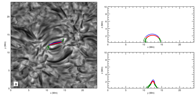
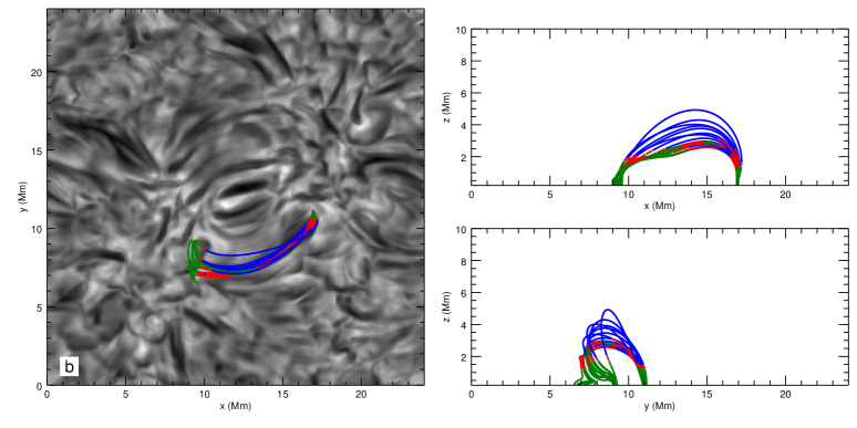
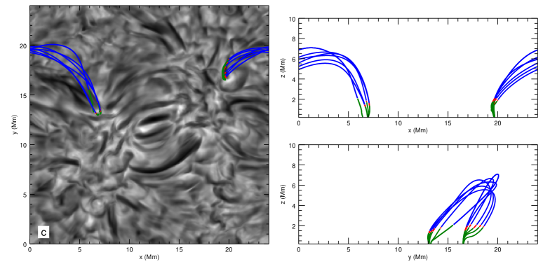
Figure 11.— Visualization of flux bundles threading through three different fibrils at $t=600$ s. The labels a, b and c correspond to the labels in Figure 9. The left panels show the top view of the field lines, superimposed on the H$\alpha$ line-core image. The panels on the right side show the $xz$ and $yz$ side views. The field lines are colour coded: the part of the field lines more than 200 km below optical depth unity in the line-core are green. The part more than 200 km above optical depth unity is blue, and the part within 200 km of optical depth unity is red. The red part of the field lines can thus be considered as visible in the H$\alpha$ line core. A movie showing the time evolution of the fibrils and field lines can be found in the online material.

In Figure 9 we show the seed points and associated field lines that we selected for further analysis. The seed points follow a number of fibrils, mostly very prominent ones, but also one fibril that appears almost transparent at $t=600$ s but is more visible before and after this moment. The $z$-coordinate of the seed point is the height of optical depth unity at that $(x,y)$ location.

The middle panel shows the part of the field lines above the height of optical depth unity. The field lines in the centre area remain low, while the other field lines reach large heights. The bottom panel shows that the field lines that point away from the centre of the domain typically reach coronal temperatures, while the central ones have chromospheric temperatures, with the latter defined as $T<17$ kK. The field lines typically end in strong photospheric field concentrations, but there are a few instances where one endpoint lies just next to a concentration. These photospheric endpoints do not visually appear to be associated with a fibril. The ending of fibril-threading field lines in photospheric magnetic field concentrations is consistent with the observational evidence that H$\alpha$ fibrils are found as if emanating from photospheric magnetic concentrations (e.g., Christopoulou et al., 2001; Tziotziou et al., 2003; Rouppe van der Voort et al., 2007), and further corroborates the idea that fibrils trace at least the horizontal components of field lines that start in photospheric magnetic field concentrations. Also note that the field lines show a strong suggestion of twist and shear, indicating that the simulated chromosphere is not in a force-free state.

Figure 11 displays for three different cases (a, b and c, also labeled in Figure 9) how the fibrils and the field lines intersect each other, and which part of the field lines can be considered visible in H$\alpha$ line-core images. The definition of visible is necessarily somewhat imprecise, because the H$\alpha$ contribution function is typically non-zero over a range of several hundred kilometers, and can even have both a chromospheric and photospheric component (Leenaarts et al., 2012). We settled for defining a point $\mathbf{r}=(x,y,z)$ on a field line as visible if it lies within 200 km from the height of optical depth unity along the same column $z_{\tau=1}(x,y)$.

The top row of panels of Figure 11 shows case a: a short fibril in the centre of the computational domain. All field lines except one form a very tight bundle, and are visible along the whole length of the fibril. The exception is the highest-reaching field line, whose seed point was on one endpoint of the fibril and can thus be considered an intermediate case between fibril and non-fibril field lines. For this fibril the assumption that fibrils trace the magnetic field in all three dimensions is true. This finding is confirmed too in the middle panel of Figure 9 where the field lines can be seen to be almost parallel to the $\tau=1$ surface. The temperature along the field lines is chromospheric. Note that the field lines show a characteristic sigmoid shape in the top view of Figure 11.

In the middle row of Figure 11 we show case b, an example of a longer fibril that does not trace the magnetic field in three dimensions. In the middle panel of Figure 9 the field lines can be seen to thread through the optical depth unity surface of the fibril at an angle. Different field lines are visible at different locations along the length of the fibril. At one end of the fibril at $(x,y)=(17,11)$ Mm the field lines all emanate from a single magnetic element, whereas at the other end the field lines connect to different magnetic elements in a patch of about $1$ Mm$\times 3$ Mm. Also these field lines remain chromospheric and do not protrude into the corona.

Finally, the bottom row of Figure 11 shows case c: field lines threading through a short fibril at $(x,y)=(20,17)$ Mm. This case is very different from the previous two. The optical depth unity surface in the fibril is nearly horizontal, and the field lines intersect this surface at large angle (more than $45^{\circ}$). In the $yz$-view at $y=17$ Mm the field lines are seen to form a fan-like structure. The field line apexes reach transition region and coronal temperatures as shown in the bottom panel of Figure 9.

6.2. Time evolution of fibrils and field lines

We now turn our attention to the question whether fibrils trace the same field line (or parts of field lines) over their lifetime. In the supplemental material we provide movies of the time evolution of the three fibrils and associated field lines shown in Figure 11. In each case the fibrils and test field lines intersect at $t=600$ s. In all three cases the field lines do not start out tracing a fibril at $t=0$ s, but instead seem to ”drift” into the fibril around $t=600$ s. After that time the field lines drift out of the fibril, while the same apparent fibril remains visible. Typically the field lines remain visible for about 100–200 s, which is of the same order as a typical observed wave period.

6.3. Analysis of the dynamics of single field lines

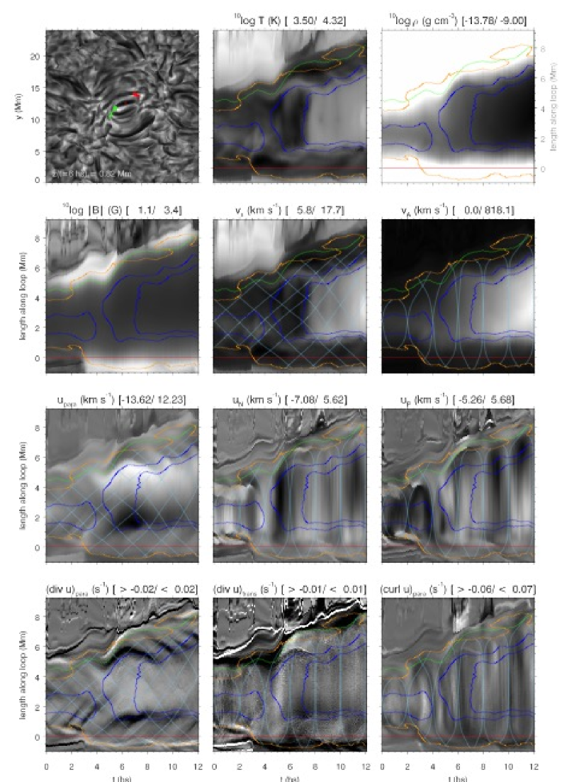
Figure 12.— Evolution of fibril-threading field line A. The upper left panel shows a top view of the computational domain, with the location of the field line at $t=0$, $t=600$ and $t=1200$ s. The location and time evolution of the footpoints are indicated in red ($\boldsymbol{b}$ points up towards the corona) and green ($\boldsymbol{b}$ points down into the convection zone). The red cross marks the location of the original seed point from which the field line and its time evolution are computed. All other panels show $st$-diagrams: the time evolution (abscissa) of quantities as function of the loop length $s$ (ordinate). The displayed quantity and its range are given above each panel. The zero point of $s$ is the intersection of the field line with the $z=0$ plane where $\boldsymbol{b}$ points upwards. It is indicated with the red line. The green curve is the $s$-coordinate of the other footpoint. Areas of the field line within the dark blue curves are visible in the H$\alpha$ line core. The orange curves indicates plasma $\beta=1$. The light blue curves are wave trajectories, i.e, a signal propagating with the wave speed along the loop would follow the indicated trajectory. The wave speed is the sound speed for the panels labeled $v_{\mathrm{s}}$, $v_{\mathrm{para}}$ and $(\mathrm{div}\,u)_{\mathrm{para}}$ and the Alfvén speed for all other panels.

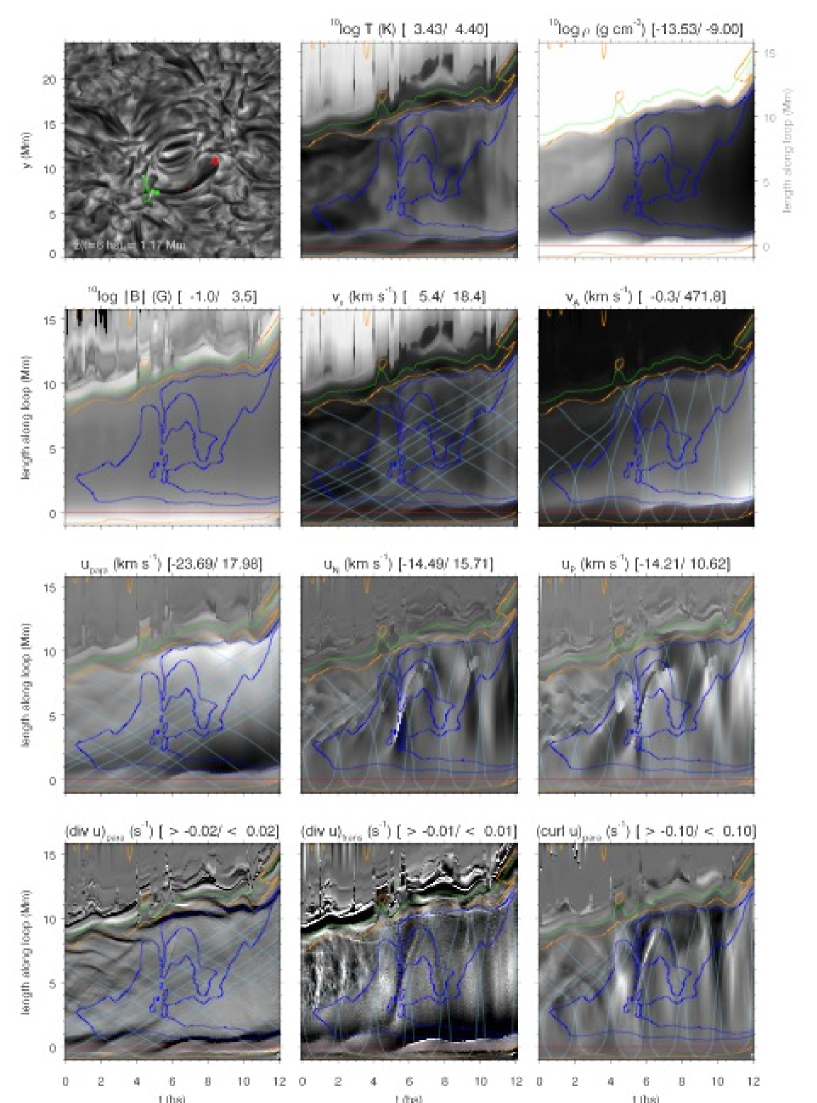
Figure 13.— Same as Figure 13 but for field line B.

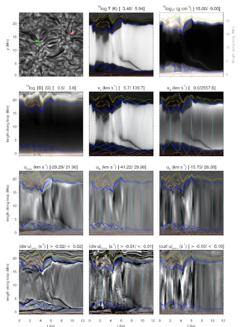
Figure 14.— Same as Figure 12 but for field line C.

Figures 12–14 show the time evolution of various quantities along the length $s$ of three fibril-threading field lines, which we label A, B and C, one from each of the three cases a,b, and c shown in Figure 9 and 11. The seed points of these field lines were in the centre of the fibrils at $t=600$ s. In the online material we provide movies of the time evolution of the 3D position of the three field lines.

The $st$-panels show the evolution of temperature $T$ and density $\rho$ in the first row; magnetic field magnitude $|\boldsymbol{B}|$, sound speed $v_{\mathrm{s}}$ and Alfvén speed $v_{\mathrm{A}}$ in the second row; plasma flow speed parallel to the field line $u_{||}=\boldsymbol{u}\cdot\boldsymbol{b}$, and along the two transverse directions $u_{\boldsymbol{P}}=\boldsymbol{u}\cdot\boldsymbol{P}$ and $u_{\boldsymbol{N}}=\boldsymbol{u}\cdot\boldsymbol{N}$ in the third row. In the fourth row we show the divergence of the plasma flow parallel to the magnetic field

$$\nabla_{||}\cdot\boldsymbol{u}=\partial u_{||}/\partial s,$$ (7)

the divergence of the flow field perpendicular to the field

$$\nabla_{\perp}\cdot\boldsymbol{u}=\nabla\cdot\boldsymbol{u}-\partial u_{||}/\partial s,$$ (8)

and the vorticity parallel to the magnetic field

$$\omega_{||}=(\nabla\times\boldsymbol{u})\cdot\boldsymbol{b}.$$ (9)

6.4. Time evolution of purely chromospheric field lines

Figure 12 shows the evolution of field line A that forms a small loop in the centre of the field-of-view. The H$\alpha$ fibril at $t=600$ s traces the field lines in this loop very well (See Section 6.1). The $\beta=1$ curves indicate that the magnetic pressure is dominant throughout the chromospheric part of the field line. The blue curves, that indicate whether the field line is visible show that the whole loop apex is visbile in H$\alpha$ for a duration $\simeq 200$ s around t=600 s. At earlier times the field line is buried too deep in the atmosphere, and at later times the loop has risen above the optical depth unity surface. The field line has typical chromospheric temperatures between 3 kK and 15 kK. As it rises over time the density of the loop apex is steadily decreasing. The magnetic field remains rather constant over time. The sound speed just depends on the square root of the temperature and varies between 5.8 and 17 km s^-1 in the chromosphere. In contrast, the Alfvén speed shows a much large variation. At the apex of the field line, it increases over time from 50 kms to 800 km s^-1as the field line rises and its density decreases. The light-blue wave-speed signal tracks illustrate this. The footpoint-to-footpoint loop crossing time for sound waves is more than 600 s, whereas the Alfvén crossing time is of the order of 100 s.

The $u_{||}$ and $\nabla_{||}\cdot\boldsymbol{u}$ panels reveal a pattern of diagonal stripes from the $\beta=1$ curve towards the loop apex. They are most clearly seen in the $\nabla_{||}\cdot\boldsymbol{u}$ panel as dark stripes, indicating compression of the plasma along the direction of the loop. They are the signature of photospherically-excited slow-mode waves that only propagate parallel to the field lines in the low-$\beta$ regime. Their slopes (and thus propagation speeds) are comparable with the sound-speed, as can be seen from comparing them with the sound-speed tracks. They are not exactly equal because of loop expansion and contraction, variation in space and time of the sound speed and the presence of background flows which modify the wave speed in the observer’s frame. Interestingly, the slow-mode waves to not cross the loop from one end to the other. Instead they typically fade before they reach the loop apex. A preliminary analysis of these waves (not shown here) shows that the radiative cooling time in the shock front is of the order of  200 s. The waves are thus damped within a sound-speed crossing time.

The $u_{||}$ panel shows another interesting phenomenon. For 600 s $\lesssim t\lesssim 800$ s it shows a white patch around $s=5$ Mm and a black patch around $s=2$ Mm. These are flows along the field line from the apex towards both footpoints and thus represent the field line draining of mass as it rises through the chromosphere.

Finally we look at the plasma motion orthogonal to the field line in the panels $u_{\boldsymbol{P}}$ and $u_{\boldsymbol{N}}$. The field line is approximately semi-circular, so $u_{\boldsymbol{P}}$ can roughly be thought of as vertical oscillation, and $u_{\boldsymbol{N}}$ as horizontal oscillation. Careful inspection of both panels shows a pattern of perturbations propagating with the Alfvén speed. The perturbations originate in the $\beta=1$ layer in both footpoints and travel all along the field line to the other footpoint with little or no apparent damping. There appears to be no wave reflection. The $\nabla_{\perp}\cdot\boldsymbol{u}$ panel shows that these perturbations are only weakly compressive. Only the perturbation around $t=5$ hs leaves a clearly recognizable imprint of weak compression orthogonal to the field line. The panel that shows $\omega_{||}$ exhibits a strong imprint of perturbations traveling with the Alfvén speed and thus provide a hint of the presence of torsional waves. However, true confirmation requires a more thorough investigation of multiple field lines.

Field line B, displayed in Figure 13, shows by and large the same features as Figure 12: the field line remains at chromospheric temperatures, it carries slow-mode waves that are damped before they cross to the other footpoint and it shows an interference pattern of transverse waves and possibly torsional waves that propagate at Alfvén speed. The biggest difference is the velocity amplitude of the transverse waves, it reaches up to 15 km s^-1 for this case, while field line A in Figure 12 showed a maximum amplitude of only 7 km s^-1.

6.5. Time evolution of a coronal field line

Field line C shown in Figure 14 behaves differently from the chromospheric field lines discussed in Section 6.4. The loop is $\sim 20$ Mm long, twice the length of the chromospheric field lines A and B. A large fraction of the loop has coronal temperatures, and only a short part close to the footpoints are chromospheric. The temperature and mass density panels show the formation of a cold, dense condensation at $t=600$ s and $s=6$ Mm. After its formation, it falls towards the chromosphere, hitting it at $t=1000$ s. These properties are similar to what is observed for coronal rain, even though the spatial scale in the simulation is much smaller (see for example Antolin & Verwichte, 2011; Antolin et al., 2012, and references therein).

Slow-mode waves propagating along this field line ($u_{\mathrm{para}}$ and $\nabla_{||}\cdot\boldsymbol{u}$ panels) do travel the whole length of the field line. This is caused by the quadratic density dependence of the radiative cooling. The wave crosses the chromosphere too fast to be completely damped. Once the wave front reaches the corona, the radiative cooling timescale goes down dramatically and becomes longer than the wave crossing time. Both loop footpoints are sources of slow-mode waves, and their lack of damping in the corona leads to an interference pattern in $u_{\mathrm{para}}$ and $\nabla_{||}\cdot\boldsymbol{u}$, but the latter is not as clear in Figure 14 because of their small compression compared to the slow-modes in the chromosphere.

The $u_{\boldsymbol{P}}$ and $u_{\boldsymbol{N}}$ again show transverse oscillations running at Alfvén speed along the field line in both directions. The vorticity panel ($\omega_{||}$) shows a hint of torsonial waves.

Note that the Alfvén crossing time for this coronal field line is $\sim 40$ s assuming a length of 20 Mm and a speed of 500 km s^-1, so that we barely resolve the propagation at the 10 s cadence of our time series.

6.6. Velocity power spectrum

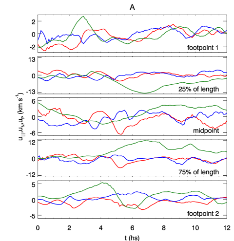
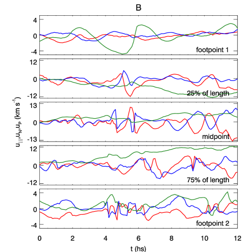
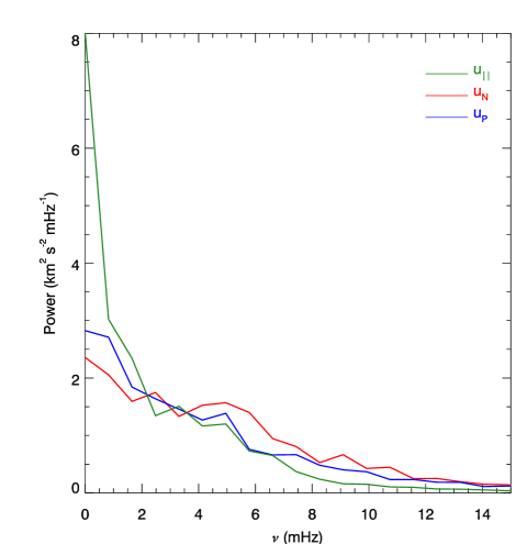
Figure 15.— Top row and bottom left: Velocities as function of time parallel ($u_{||}$, green) and perpendicular to the magnetic field ($u_{N}$ in red and $u_{P}$ in blue) along the three field lines A,B,C. Subpanels show the velocities at different locations along the field line, where 100% means the length from one footpoint to the other. Lower right panel: power spectrum of the velocity components at the loop apexes averaged over all 80 field lines. Only positive frequencies are shown.

For completeness we further quantify the flow velocities along the field lines A, B and C in Figure 15. The velocities increase from the footpoints towards the field line midpoints. The parallel and perpendicular velocities have similar magnitude at similar locations along the field lines. The parallel velocity $u_{||}$ varies on longer time scales than the two perpendicular components. This slow variation is associated with field lines loading and draining of mass.

In the lower right panel of Figure 15 we show the power spectrum of the three velocity components at the midpoint of the field lines (i.e., halfway between the footpoints). These power spectra were obtained by computing a power spectrum of each velocity component at 11 points equally spaced between 40% and 60% of the length of each field line. For each velocity component these spectra were then averaged over the 11 points and over all field lines. The averaging over 11 points was done to beat down the noise.

The high power of $u_{||}$ at the lowest resolvable frequencies again represents loop mass loading and draining. There are weak maxima of power at 5 mHz in all three velocity components. Given the limited sample size and duration of the time series, we do not know whether these peaks are significant. If they are, they might correspond to the familiar 3-minute oscillations. The typical power of 1-2 km² s^-2 mHz^-1 are the same order of magnitude as those found based on fibril oscillations in Figure 4 of Morton et al. (2014).

7. Discussion and conclusions

In this paper we investigated the relation between fibrils, dark elongated features seen in images of the Sun taken in the core of the chromospheric H$\alpha$ line, and magnetic field lines that thread through the chromosphere. We compared synthetic H$\alpha$ imagery computed from an RMHD simulation of an enhanced network area on the Sun with observations. The simulation behaves similar in terms of intensity contrast, Doppler shifts and time evolution. A difference is that the fibrils in the synthetic imagery appear as a cross between active region and quiet Sun fibrils. Comparison of the properties of the oscillatory behaviour of fibrils in the synthetic line core imagery with those observed by Kuridze et al. (2012, 2013) and Morton et al. (2014) showed that the simulated fibrils have periods, amplitudes, and phase speeds consistent with the observations.

We then proceeded with an extensive analysis of the relation between fibrils and fibril-threading field lines in our simulation. This relation is one of complex interplay between field line dynamics on the one hand, and the formation of the H$\alpha$ line on the other hand.

The evolution of the field lines themselves is extremely intricate. The slow motion of their footpoints by the evolving granulation pattern leads to a slow migration of the field line paths through the 3D computational volume on time scales of several hundred seconds. In our examples, the field lines tend to evolve from lower to higher-reaching loops. The field lines can in general thus not be thought of as a static background along which waves propagate.

Footpoint buffeting by radial box oscillations (corresponding to solar $p$-modes) and granules cause excitation of different types of waves.

We identified the presence of compressive longitudinal slow-mode waves, that steepen to shocks at chromospheric heights and propagate with speeds close to the sound speed. The plasma $\beta$ is smaller than unity along the field lines, so that these waves propagate parallel to the field lines. If these field lines are close to horizontal, then the large angle of the field lines with the vertical combined with the frozen in condition might prevent the loop from draining quickly. For those field lines that do not reach coronal temperatures, the slow-modes are typically damped before the wave front reaches the other footpoint. This damping is reduced once the shock front reaches to the corona, and such waves travel through the corona to the other footpoint.

The second wave type that we identified is a nearly-incompressible transverse wave that propagates with the Alfvén speed. These waves are ubiquitously present in all investigated field lines along both transverse Frenet-Serret directions ($\boldsymbol{N}$ and $\boldsymbol{P}$). They have maximum velocity amplitudes of 5–20 km s^-1. The field lines typically carry waves travelling in both directions along the field. We do not find evidence of standing waves or reflection. We also find signal propagating with Alfvén speed in the vorticity parallel to the magnetic field $\omega_{||}$. Without further analysis we cannot confirm whether the vorticity signal indicates a torsional wave-like phenomenon, such as reported in De Pontieu et al. (2012, 2014) or whether it is caused by a form of motion comparable to helical kink waves in idealised linear wave analysis (Zaqarashvili & Skhirtladze, 2008). In the latter case they merely represent another way to view the transverse waves along $\boldsymbol{N}$ and $\boldsymbol{P}$.

Our field line based analysis approach only brings forward waves that travel parallel to the magnetic field. The third classical MHD wave, the fast mode, can propagate at an angle to the magnetic field and can therefore not be easily identified in our field-line based approach. While these waves are present in the simulation, we did not try to identify them.

From an H$\alpha$ line formation point of view, the fibrils are dark elongated features. They appear dark because they reach optical depth unity at larger height than their surroundings. The H$\alpha$ opacity is relatively insensitive to temperature, and depends mainly on mass density. The location of optical depth unity in the line core is therefore roughly equal to the height were the integrated mass density (column mass) along the line of sight reaches a certain value ($3\times 10^{-5}$ g cm^-3 in the analysis by Leenaarts et al. (2012)). Whether (a part of) a given magnetic field line is visible as part of a fibril therefore depends on the mass density along the field line, and the column mass density above it. The column mass density at which optical depth unity is located is just set by the characteristics of the radiative transfer in the H$\alpha$ line, and has no special significance in terms of properties of the atmosphere.

The combination of the movement of field lines through the atmosphere and the filling and draining of mass along field lines thus determines whether a part of a given field line is visible in H$\alpha$ line core images. From the analysis of the time evolution of the fibrils and field lines in the movies associated with Figure 11 we find that a fibril in our simulation tracks the same set of field lines for about 200 s. The fibrils themselves keep their identity typically for a longer time (500 s to 1000 s). In this respect our simulation behaves more like the active region fibrils analysed in Figure 2 of Morton et al. (2014), where fibrils retain their identity for about 500 s, whereas the quiet Sun fibrils are identifiable over shorter periods (200 s – 300 s). A big open question is whether true solar field lines migrate through the atmosphere as fast as in our simulation.

Returning to the assumptions behind using fibril oscillations in coronal seismology in Section 1, we find the following: The simulation shows instances where fibrils outline single magnetic field lines (top row of Figure 9, but also examples where the fibril roughly follows a field line bundle, but different field lines are visible at different locations along the fibril (middle row of Figure 9) and examples where the fibril intersects field lines at a large angle (bottom row of Figure 9). In the latter case the fibril does not follow single field lines at all. Whether a given fibril traces single field lines cannot be determined from the H$\alpha$ observations alone. The simulation also shows that field lines evolve in time though the computational domain, and do not intersect a fibril for longer than $~{}200$ s. This is comparable to typical transverse wave periods.

We conclude that our simulation only partially supports the assumptions typically made in chromospheric seismology. There will be instances where a fibril indeed traces out a single field line over more than one transverse-wave period, but this cannot be expected to be generally true. We therefore urge caution when interpreting results obtained from seismology, as they might contain systematic biases caused by the partial mapping of fibril oscillations to actual plasma and field line motion.

The work presented in the manuscript also leads to a number of intriguing new questions: What are the precise excitation mechanisms of the transverse waves along fibril threading field lines? How can fibrils retain their identity for a time that is longer than the time that they intersect the same field lines? How much of the transverse and longitudinal wave energy is deposited in the chromosphere? What is the dissipation mechanism of the waves? How exactly is mass loaded into fibril-threading field lines? Which forces act to prevent the mass-loaded fibrils to sink back deeper into the atmosphere? Why are fibrils in active regions narrower than in the quiet Sun? We intend to address these questions in future publications.

References

- Antolin & Verwichte (2011) Antolin, P. & Verwichte, E. 2011, ApJ, 736, 121
- Antolin et al. (2012) Antolin, P., Vissers, G., & Rouppe van der Voort, L. 2012, Sol. Phys., 280, 457
- Christopoulou et al. (2001) Christopoulou, E. B., Georgakilas, A. A., & Koutchmy, S. 2001, Sol. Phys., 199, 61
- Clyne et al. (2007) Clyne, J., Mininni, P., Norton, A., & Rast, M. 2007, New Journal of Physics, 9, 301
- de la Cruz Rodríguez et al. (2014) de la Cruz Rodríguez, J., Löfdahl, M., Sütterlin, P., Hillberg, T., & Rouppe van der Voort, L. 2014, ArXiv e-prints
- de la Cruz Rodríguez & Socas-Navarro (2011) de la Cruz Rodríguez, J. & Socas-Navarro, H. 2011, A&A, 527, L8
- De Pontieu et al. (2012) De Pontieu, B., Carlsson, M., Rouppe van der Voort, L. H. M., et al. 2012, ApJ, 752, L12
- De Pontieu et al. (2007) De Pontieu, B., Hansteen, V. H., Rouppe van der Voort, L., van Noort, M., & Carlsson, M. 2007, ApJ, 655, 624
- De Pontieu et al. (2014) De Pontieu, B., Rouppe van der Voort, L., McIntosh, S. W., et al. 2014, Science, 346, D315
- Dresselhaus & Tabor (1992) Dresselhaus, E. & Tabor, M. 1992, Journal of Fluid Mechanics, 236, 415
- Frenet (1852) Frenet, F. 1852, Journal de mathématiques pures et appliquées 1re série, 17, 437
- Gudiksen et al. (2011) Gudiksen, B. V., Carlsson, M., Hansteen, V. H., et al. 2011, A&A, 531, A154
- Hansteen et al. (2006) Hansteen, V. H., De Pontieu, B., Rouppe van der Voort, L., van Noort, M., & Carlsson, M. 2006, ApJ, 647, L73
- Jing et al. (2011) Jing, J., Yuan, Y., Reardon, K., et al. 2011, ApJ, 739, 67
- Kuridze et al. (2012) Kuridze, D., Morton, R. J., Erdélyi, R., et al. 2012, ApJ, 750, 51
- Kuridze et al. (2013) Kuridze, D., Verth, G., Mathioudakis, M., et al. 2013, ApJ, 779, 82
- Leenaarts & Carlsson (2009) Leenaarts, J. & Carlsson, M. 2009, in Astronomical Society of the Pacific Conference Series, Vol. 415, The Second Hinode Science Meeting: Beyond Discovery-Toward Understanding, ed. B. Lites, M. Cheung, T. Magara, J. Mariska, & K. Reeves, 87
- Leenaarts et al. (2012) Leenaarts, J., Carlsson, M., & Rouppe van der Voort, L. 2012, ApJ, 749, 136
- Leenaarts et al. (2013a) Leenaarts, J., Pereira, T. M. D., Carlsson, M., Uitenbroek, H., & De Pontieu, B. 2013a, ApJ, 772, 89
- Leenaarts et al. (2013b) Leenaarts, J., Pereira, T. M. D., Carlsson, M., Uitenbroek, H., & De Pontieu, B. 2013b, ApJ, 772, 90
- Longcope (2005) Longcope, D. W. 2005, Living Reviews in Solar Physics, 2, 7
- Morton et al. (2013) Morton, R. J., Verth, G., Fedun, V., Shelyag, S., & Erdélyi, R. 2013, ApJ, 768, 17
- Morton et al. (2014) Morton, R. J., Verth, G., Hillier, A., & Erdélyi, R. 2014, ApJ, 784, 29
- Pereira et al. (2013) Pereira, T. M. D., Leenaarts, J., De Pontieu, B., Carlsson, M., & Uitenbroek, H. 2013, ApJ, 778, 143
- Rosenthal et al. (2002) Rosenthal, C. S., Bogdan, T. J., Carlsson, M., et al. 2002, ApJ, 564, 508
- Rouppe van der Voort & de la Cruz Rodríguez (2013) Rouppe van der Voort, L. & de la Cruz Rodríguez, J. 2013, ApJ, 776, 56
- Rouppe van der Voort et al. (2007) Rouppe van der Voort, L. H. M., De Pontieu, B., Hansteen, V. H., Carlsson, M., & van Noort, M. 2007, ApJ, 660, L169
- Rutten et al. (2008) Rutten, R. J., van Veelen, B., & Sütterlin, P. 2008, Sol. Phys., 251, 533
- Scharmer et al. (2003a) Scharmer, G. B., Bjelksjo, K., Korhonen, T. K., Lindberg, B., & Petterson, B. 2003a, in Innovative Telescopes and Instrumentation for Solar Astrophysics. Edited by Stephen L. Keil, Sergey V. Avakyan . Proceedings of the SPIE, Volume 4853, pp. 341-350 (2003)., 341–350
- Scharmer et al. (2003b) Scharmer, G. B., Dettori, P. M., Lofdahl, M. G., & Shand, M. 2003b, in Innovative Telescopes and Instrumentation for Solar Astrophysics. Edited by Stephen L. Keil, Sergey V. Avakyan . Proceedings of the SPIE, Volume 4853, pp. 370-380 (2003)., 370–380
- Scharmer et al. (2008) Scharmer, G. B., Narayan, G., Hillberg, T., et al. 2008, ApJ, 689, L69
- Serret (1851) Serret, J.-A. 1851, Journal de mathématiques pures et appliquées 1re série, 16, 499
- Simon & Leighton (1964) Simon, G. W. & Leighton, R. B. 1964, ApJ, 140, 1120
- Simon & White (1966) Simon, G. W. & White, O. R. 1966, ApJ, 143, 38
- Socas-Navarro & Uitenbroek (2004) Socas-Navarro, H. & Uitenbroek, H. 2004, ApJ, 603, L129
- Stein & Nordlund (2001) Stein, R. F. & Nordlund, Å. 2001, ApJ, 546, 585
- Tomczyk & McIntosh (2009) Tomczyk, S. & McIntosh, S. W. 2009, ApJ, 697, 1384
- Tsiropoula et al. (2012) Tsiropoula, G., Tziotziou, K., Kontogiannis, I., et al. 2012, Space Sci. Rev., 169, 181
- Tziotziou et al. (2003) Tziotziou, K., Tsiropoula, G., & Mein, P. 2003, A&A, 402, 361
- Štěpán et al. (2012) Štěpán, J., Trujillo Bueno, J., Carlsson, M., & Leenaarts, J. 2012, ApJ, 758, L43
- van Doorsselaere et al. (2009) van Doorsselaere, T., Verwichte, E., & Terradas, J. 2009, Space Sci. Rev., 149, 299
- van Noort et al. (2005) van Noort, M., Rouppe van der Voort, L., & Löfdahl, M. G. 2005, Sol. Phys., 228, 191
- Vernazza et al. (1981) Vernazza, J. E., Avrett, E. H., & Loeser, R. 1981, ApJS, 45, 635
- Wiegelmann et al. (2008) Wiegelmann, T., Thalmann, J. K., Schrijver, C. J., De Rosa, M. L., & Metcalf, T. R. 2008, Sol. Phys., 247, 249
- Zaqarashvili & Skhirtladze (2008) Zaqarashvili, T. V. & Skhirtladze, N. 2008, ApJ, 683, L91