Production of the $Y(4260)$ state in B meson decay

Abstract

We calculate the branching ratio for the production of the meson $Y(4260)$ in the decay $B^{-}\to Y(4260)K^{-}$. We use QCD sum rules approach and we consider the $Y(4260)$ to be a mixture between charmonium and exotic tetraquark, $[\bar{c}\bar{q}][qc]$, states with $J^{PC}=1^{--}$. Using the value of the mixing angle determined previously as: $\theta=(53.0\pm 0.5)^{\circ}$, we get the branching ratio $\mathcal{B}(B\to Y(4260)K)=(1.34\pm 0.47)\times 10^{-6}$, which allows us to estimate an interval on the branching fraction $3.0\times 10^{-8}<{\mathcal{B}}_{{}_{Y}}<1.8\times 10^{-6}$ in agreement with the experimental upper limit reported by Babar Collaboration.

The $Y(4260)$ state was first observed by BaBar collaboration in the $e^{+}e^{-}$ annihilation through initial state radiation babar1 , and it was confirmed by CLEO and Belle collaborations yexp . The $Y(4260)$ was also observed in the $B^{-}\to Y(4260)K^{-}\to J/\Psi\pi^{+}\pi^{-}K^{-}$ decay babary2 , and CLEO reported two additional decay channels: $J/\Psi\pi^{0}\pi^{0}$ and $J/\Psi K^{+}K^{-}$ yexp . The $Y(4260)$ is one of the many charmonium-like state, called $X,~{}Y$ and $Z$ states, recently observed in $e^{+}e^{-}$ collisions by BaBar and Belle collaborations that do not fit the quarkonia interpretation. The production mechanism, masses, decay widths, spin-parity assignments and decay modes of these states have been discussed in some reviews Zhu:2007wz ; Nielsen:2009uh ; Brambilla:2010cs ; Nielsen:2014mva . The $Y(4260)$ is particularly interesting because some new states have been identified in the decay channels of the $Y(4260)$, like the $Z_{c}^{+}(3900)$. The $Z_{c}^{+}(3900)$ was first observed by the BESIII collaboration in the $(\pi^{\pm}J/\psi)$ mass spectrum of the $Y(4260)\to J/\psi\pi^{+}\pi^{-}$ decay channel Ablikim:2013mio . This structure, was also observed at the same time by the Belle collaboration Liu:2013dau and was confirmed by the authors of Ref.  Xiao:2013iha using CLEO-c data.

The decay modes of the $Y(4260)$ into $J/\psi$ and other charmonium states indicate the existence of a $\bar{c}c$ in its content. However, the attempts to classify this state in the charmonium spectrum have failed since the $\Psi(3S),~{}\Psi(2D)$ and $\Psi(4S)$ $c\bar{c}$ states have been assigned to the well established $\Psi(4040),~{}\Psi(4160),~{}$ and $\Psi(4415)$ mesons respectively, and the prediction from quark models for the $\Psi(3D)$ state is 4.52 GeV. Therefore, the mass of the $Y(4260)$ is not consistent with any of the $1^{--}$ $c\bar{c}$ states Zhu:2007wz ; Nielsen:2009uh .

Some theoretical interpretations for the $Y(4260)$ are: tetraquark state tetraquark , hadronic $D_{1}D$, $D_{0}D^{*}$ molecule Ding , $\chi_{c1}\omega$ molecule Yuan , $\chi_{c1}\rho$ molecule liu , $J/\psi f_{0}(980)$ molecule oset , a hybrid charmonium zhu , a charm-baryonium Qiao , a cusp eef1 ; eef2 ; eef3 , etc. Within the available experimental information, none of these suggestions can be completely ruled out. However, there are some calculations, within the QCD sum rules (QCDSR) approach Nielsen:2009uh ; svz ; rry ; SNB , that can not explain the mass of the $Y(4260)$ supposing it to be a tetraquark state rapha , or a $D_{1}D$, $D_{0}D^{*}$ hadronic molecule rapha , or a $J/\psi f_{0}(980)$ molecular state Albuquerque:2011ix .

In the framework of the QCDSR the mass and the decay width, in the channel $J/\psi\pi\pi$, of the $Y(4260)$ were computed with good agreement with data, considering it as a mixing between two and four-quark states Dias:2012ek . The mixing is done at the level of the hadronic currents and, physically, this corresponds to a fluctuation of the $c\overline{c}$ state where a gluon is emitted and subsequently splits into a light quark-antiquark pair, which lives for some time and behaves like a tetraquark-like state. The same approach was applied to the $X(3872)$ state and good agreement with the data were obtained for its mass and the decay width into $J/\psi\pi\pi$ x3872mix , its radiative decay x3872rad , and also in the $X(3872)$ production rate in $B$ decay x3872prod .

In this work we will focus on the production of the $Y(4260)$, using the mixed two-quark and four-quark prescription of Ref. Dias:2012ek to perform a QCDSR analysis of the process $B^{-}\to Y(4260)K^{-}$. The experimental upper limit on the branching fraction for such a production in $B$ meson decay has been reported by BaBar Collaboration babary2 , with $95\%$ C.L.,

$${\mathcal{B}}_{{}_{Y}}<\!2.9\times 10^{-5}$$ (1)

where ${\mathcal{B}}_{{}_{Y}}\equiv{\mathcal{B}}(B^{-}\!\!\to\!K^{-}Y(4260),Y(4260)\!\to\!J/\psi\pi^{+}\pi^{-})$.

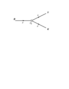
Figure 1: The process for production of the $Y(4260)$ state in B meson decay, mediated by an effective vertex operator ${\mathcal{O}}_{2}$.

The process $B\to Y(4260)K$ occurs via weak decay of the $b$ quark, while the $u$ quark is a spectator. The $Y$ meson as a mixed state of tetraquark and charmonium interacts via $\bar{c}c$ component of the weak current. In effective theory, at the scale $\mu\sim m_{b}\ll m_{W}$, the weak decay is treated as a four-quark local interaction described by the effective Hamiltonian (see Fig. 1):

$${\mathcal{H}}_{W}=\frac{G_{F}}{\sqrt{2}}V_{cb}V_{cs}^{*}\left[\left(C_{2}(\mu)+\frac{C_{1}(\mu)}{3}\right){\mathcal{O}}_{2}+\cdots\right]\,,$$ (2)

where $V_{ik}$ are CKM matrix elements, $C_{1}(\mu)$ and $C_{2}(\mu)$ are short distance Wilson coefficients computed at the renormalization scale $\mu\sim{\mathcal{O}}(m_{b})$. The four-quark effective operator is ${\mathcal{O}}_{2}=J_{\mu}^{(\bar{c}c)}J_{\mu}^{W}$, with

$$J_{\mu}^{W}=\bar{s}\Gamma_{\mu}b\,,\quad J_{\mu}^{(\bar{c}c)}=\bar{c}\Gamma_{\mu}c\,,$$ (3)

and $\Gamma_{\mu}=\gamma_{\mu}(1-\gamma_{5})$.

Using factorization, the decay amplitude of the process is calculated from the Hamiltonian (2), by splitting the matrix element in two pieces:

$${\mathcal{M}} = i\frac{G_{F}}{\sqrt{2}}V_{cb}V_{cs}^{*}\left(C_{2}+\frac{C_{1}}{3}\right)$$ (4)

$$\times \langle B(p)|J_{\mu}^{W}|K(p^{\prime})\rangle\langle Y(q)|J^{\mu(\bar{c}c)}|0\rangle,$$

where $p=p^{\prime}+q$. Following Ref. x3872prod , the matrix elements in Eq. (4) are parametrized as:

$$\langle Y(q)|J_{\mu}^{(\bar{c}c)}|0\rangle=\lambda_{W}\epsilon^{\ast}_{\mu}(q)\,,$$ (5)

and

$$\langle B(p)|J_{\mu}^{W}|K(p^{\prime})\rangle=f_{+}(q^{2})(p_{\mu}+p_{\mu}^{\prime})+f_{-}(q^{2})(p_{\mu}-p_{\mu}^{\prime})\,.$$ (6)

The parameter $\lambda_{W}$ in (5) gives the coupling between the current $J_{\mu}^{(\bar{c}c)}$ and the $Y$ state. The form factors $f_{\pm}(q^{2})$ describe the weak transition $B\to K$. Hence we can see that the factorization of the matrix element describes the decay as two separated sub-processes.

The decay width for the process $B^{-}\to Y(4260)K^{-}$ is given by

$$\Gamma(B\to YK)=\frac{|{\mathcal{M}}|^{2}}{16\pi m_{B}^{3}}\sqrt{\lambda(m_{B}^{2},m_{K}^{2},m_{Y}^{2})},$$ (7)

with $\lambda(x,y,z)=x^{2}+y^{2}+z^{2}-2xy-2xz-2yz$. The invariant amplitude squared can be obtained from (4), using (5) and (6):

$$|\mathcal{M}|^{2} = \frac{G_{F}^{2}}{2m_{Y}^{2}}|V_{cb}V_{cs}|^{2}\left(C_{2}+\frac{C_{1}}{3}\right)^{2}$$ (8)

$$\times \lambda(m_{B}^{2},m_{K}^{2},m_{Y}^{2})\lambda_{W}^{2}f_{+}^{2}\,.$$

The coupling constant $f_{+}$ was determined in Ref.x3872prod through extrapolation of the form factor $f_{+}(Q^{2})$ to the meson pole $Q^{2}=-m_{Y}^{2}$, using the QCDSR approach for the three-point correlator bcnn :

$$\Pi_{\mu}(p,p^{\prime}) = \!\!\int d^{4}x\,d^{4}y\,e^{i(p^{\prime}\cdot x-\,p\cdot y)}\langle 0|T\{J_{\mu}^{W}(0)\times$$ (9)

$$\times J_{K}(x)J^{\dagger}_{B}(y)\}|0\rangle,$$

where the weak current, $J^{W}_{\mu}$, is defined in (3) and the interpolating currents of the $B$ and $K$ pseudoscalar mesons are:

$$J_{K}=i\,\bar{u}_{a}\gamma_{5}s_{a}\,,\quad J_{B}=i\,\bar{u}_{a}\gamma_{u}b_{a}\,.$$ (10)

The obtained result for the form factor was x3872prod :

$$f_{+}(Q^{2})=\frac{(17.55\pm 0.04)\mbox{ GeV}^{2}}{(105.0\pm 1.8)\mbox{ GeV}^{2}+Q^{2}}\,.$$ (11)

For the decay width calculation, we need the value of the form factor at $Q^{2}=-m_{Y}^{2}$, where $m_{Y}$ is the mass of the $Y(4260)$ meson. Using $m_{Y}=(4251\pm 9)\mbox{ MeV}$ pdg we get:

$$f_{+}(Q^{2})|_{Q^{2}=-m_{Y}^{2}}=0.206\pm 0.004\,.$$ (12)

The parameter $\lambda_{W}$ can also be determined using the QCDSR approach for the two-point correlator:

$$\Pi_{\mu\nu}(q)=i\int d^{4}y~{}e^{iq\cdot y}\langle 0|T\{J_{\mu}^{Y}(y)J_{\nu}^{(\bar{c}c)}(0)\}|0\rangle\,,$$ (13)

where the current $J_{\nu}^{(\bar{c}c)}$ is defined in (3). For the $Y$ meson we will follow Dias:2012ek and consider a mixed charmonium-tetraquark current:

$$J_{\mu}^{Y}=\sin\theta\>J_{\mu}^{(4)}+\cos\theta\>J_{\mu}^{(2)},$$ (14)

where

$$J_{\mu}^{(4)} = \frac{\epsilon_{abc}\epsilon_{dec}}{\sqrt{2}}\Big{[}(q_{a}^{T}C\gamma_{5}c_{b})(\bar{q}_{d}\gamma_{\mu}\gamma_{5}C\bar{c}_{e}^{T})+$$ (15)

$$~{}+(q_{a}^{T}C\gamma_{5}\gamma_{\mu}c_{b})(\bar{q}_{d}\gamma_{5}C\bar{c}_{e}^{T})\Big{]},$$

$$J_{\mu}^{(2)}=\frac{1}{\sqrt{2}}\langle\bar{q}q\rangle\>\Big{(}\bar{c}_{a}\gamma_{\mu}c_{a}\Big{)}~{}\equiv~{}\frac{1}{\sqrt{2}}\langle\bar{q}q\rangle\>J_{\mu}^{{}^{\prime}(2)}~{}.$$ (16)

In Eq. (14), $\theta$ is the mixing angle that was determined in Dias:2012ek to be: $\theta=(53.0\pm 0.5)^{0}$.

Inserting the currents (3) and (14) in the correlator we have in the OPE side of the sum rule

$$\Pi^{\mathrm{OPE}}_{\mu\nu}(q) = \sin\theta\,\Pi^{4,2}_{\mu\nu}(q)+\frac{\langle\bar{q}q\rangle}{\sqrt{2}}\cos\theta\,\Pi^{2,2}_{\mu\nu}(q)\,,$$ (17)

where

$$\Pi^{4,2}_{\mu\nu}(q) = i\int d^{4}y~{}e^{iq\cdot y}\langle 0|T\{J_{\mu}^{(4)}(y)J_{\nu(\bar{c}c)}(0)\}|0\rangle$$

$$\Pi^{2,2}_{\mu\nu}(q) = i\int d^{4}y~{}e^{iq\cdot y}\langle 0|T\{J_{\mu}^{{}^{\prime}(2)}(y)J_{\nu(\bar{c}c)}(0)\}|0\rangle\,.$$ (18)

Only the vector part of the current $J_{\nu}^{(\bar{c}c)}$ contributes to the correlators in Eq. (18). Therefore, these correlators are the same as the ones calculated in Ref. Dias:2012ek for the mass of the $Y(4260)$.

Table 1: QCD input parameters.

Parameters	Values
$\overline{m}_{c}$	$(1.23-1.47)\mbox{ GeV}$
$\langle\bar{q}q\rangle$	$-(0.23\pm 0.03)^{3}\mbox{ GeV}^{3}$
$\langle g_{s}^{2}G^{2}\rangle$	$(0.88\pm 0.25)~{}\mbox{ GeV}^{4}$
$m_{0}^{2}\equiv\langle\bar{q}Gq\rangle/\langle\bar{q}q\rangle$	$(0.8\pm 0.1)~{}\mbox{ GeV}^{2}$

To evaluate the phenomenological side we insert intermediate states of the $Y$:

$$\Pi_{\mu\nu}^{phen}(q) = \frac{i}{q^{2}-m_{Y}^{2}}\langle 0|J^{Y}_{\mu}|Y(q)\rangle\langle Y(q)|J^{(\bar{c}c)}_{\nu}|0\rangle\,,$$ (19)

$$= \frac{i\lambda_{Y}\lambda_{W}}{Q^{2}+m_{Y}^{2}}\left(g_{\mu\nu}-\frac{q_{\mu}q_{\nu}}{m_{Y}^{2}}\right)$$

where $q^{2}=-Q^{2}$, and we have used the definition (5) and

$$\langle 0|J^{Y}_{\mu}|Y(q)\rangle=\lambda_{Y}\epsilon_{\mu}(q)\,.$$ (20)

The parameter $\lambda_{Y}$, that defines the coupling between the current $J^{Y}_{\mu}$ and the $Y$ meson, was determined in Ref. Dias:2012ek to be: $\lambda_{Y}=(2.00\pm 0.23)\times 10^{-2}~{}\mbox{ GeV}^{5}$.

As usual in the QCDSR approach, we perform a Borel transform to $Q^{2}\to M_{B}^{2}$ to improve the matching between both sides of the sum rules. After performing the Borel transform in both sides of the sum rule we get in the $g_{\mu\nu}$ structure:

$$\lambda_{W}\lambda_{Y}e^{-\frac{m_{Y}^{2}}{M_{B}^{2}}}=\frac{\sin\theta}{\sqrt{2}}\,\Pi^{4,2}(M_{B}^{2})+\frac{\langle\bar{q}q\rangle}{\sqrt{2}}\cos\theta\,\Pi^{2,2}(M_{B}^{2})~{}~{}~{}~{}~{}~{}$$ (21)

where the invariant functions $\Pi^{2,2}(M_{B}^{2})$ and $\Pi^{4,2}(M_{B}^{2})$ are written in terms of a dispersion relation,

$$\Pi(M_{B}^{2})=\int\limits_{4m_{c}^{2}}^{\infty}\!ds~{}e^{-s/M_{B}^{2}}\>\rho(s)~{}~{},$$ (22)

with their respective spectral densities $\rho^{2,2}(s)$ and $\rho^{4,2}(s)$ given in Appendix.

We perform the calculation of the coupling parameter $\lambda_{W}$ using the same values for the masses and QCD condensates as in Ref. Dias:2012ek which are listed in Table 1. To be consistent with the calculation of $\lambda_{Y}$ we also use the same region in the threshold parameter $s_{0}$ as in Ref. Dias:2012ek : $\sqrt{s_{0}}=(4.70\pm 0.10)$ GeV. As one can see in Fig. 2, the region where we get $M_{B}^{2}$-stability is given by: $(8.0\leq M_{B}^{2}\leq 25.0)\mbox{ GeV}^{2}$.

Taking into account the variation in the Borel mass parameter, in the continuum threshold, in the quark condensate, in the coupling constant $\lambda_{Y}$ and in the mixing angle $\theta$, the result for the $\lambda_{W}$ parameter is:

$$\lambda_{W}=(0.90\pm 0.32)\mbox{ GeV}^{2}\,.$$ (23)

Thus we can calculate the decay width in Eq. (7) by using the values of $f_{+}(-M_{Y}^{2})$ and $\lambda_{W}$, determined in Eqs. (12) and (23). The branching ratio is evaluated dividing the result by the total width of the $B$ meson $\Gamma_{\mathrm{tot}}=4.280\times 10^{-4}\>\mbox{eV}$:

$$\mathcal{B}(B\to Y(4260)K)=(1.34\pm 0.47)\times 10^{-6}\,,$$ (24)

where we have used the CKM parameters $V_{cs}=1.023$, $V_{cb}=40.6\times 10^{-3}$ pdg , and the Wilson coefficients $C_{1}(\mu)=1.082$, $C_{2}(\mu)=-0.185$, computed at $\mu=m_{b}$ and $\bar{\Lambda}_{\mathrm{MS}}=225\mbox{ MeV}$ buras .

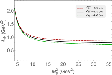
Figure 2: The coupling parameter $\lambda_{W}$ as a function of $M_{B}^{2}$, for different values of the continuum threshold.

In order to compare the branching ratio in Eq. (24) with the branching fraction obtained experimentally in Eq. (1), we might use the results found in Ref. Dias:2012ek :

$$\mathcal{B}(Y(4260)\to J/\psi\>\pi^{+}\pi^{-})=(4.3\pm 0.9)\times 10^{-2}\,,$$ (25)

and then, considering the uncertainties, we can estimate ${\mathcal{B}}_{{}_{Y}}>\!3.0\times 10^{-8}$. However, it is important to notice that the authors in Ref. Dias:2012ek have considered two pions in the final state coming only from intermediate states, e.g. $\sigma$ and $f_{0}(980)$ mesons, which could indicate that the result in Eq. (25) can be underestimated. In this sense, considering that the main decay channel observed for the $Y(4260)$ state is into $J/\psi\>\pi^{+}\pi^{-}$, we would naively expect that the branching ratio into this channel could also be $\mathcal{B}(Y(4260)\to J/\psi\>\pi^{+}\pi^{-})\sim 1.0$, which would lead to the following result, ${\mathcal{B}}_{{}_{Y}}<\!1.8\times 10^{-6}$. Therefore, we obtain an interval on the branching fraction

$$3.0\times 10^{-8}<{\mathcal{B}}_{{}_{Y}}<1.8\times 10^{-6}$$ (26)

which is in agreement with the experimental upper limit reported by Babar Collaboration given in Eq. (1). In general the experimental evaluation of the branching fraction takes into account additional factors related to the numbers of reconstructed events for the final state ($J/\psi\>\pi^{+}\pi^{-}\>K$), for the reference process ($B\to Y(4260)\>K$), and for the respective reconstruction efficiencies. However, since such information has not been provided in Ref. babary2 , we have neglected these factors in the calculation of the branching fraction ${\mathcal{B}}_{Y}$. Therefore, the comparison of our result with the experimental result could be affected by these differences.

In conclusion, we have used the QCDSR approach to evaluate the production of the $Y(4260)$ state, considered as a mixed charmonium-tetraquark state, in the decay $B\to YK$. Using the factorization hypothesis, we find that the sum rules result in Eq. (24), is compatible with the experimental upper limit. Our result can be interpreted as a lower limit for the branching ratio, since we did not considered the non-factorizable contributions.

Our result was obtained by considering the mixing angle in Eq. (14) in the range $\theta=(53.0\pm 0.5)^{0}$. This angle was determined in Ref. Dias:2012ek where the mass and the decay width of the $Y(4260)$ in the channel $J/\psi\pi^{+}\pi^{-}$ were determined in agreement with experimental values. Therefore, since there is no new free parameter in the present analysis, the result presented here strengthens the conclusion reached in Dias:2012ek that the $Y(4260)$ is probably a mixture between a $c\bar{c}$ state and a tetraquark state.

As discussed in x3872prod , it is not simple to determine the charmonium and the tetraquark contribution to the state described by the current in Eq. (14). From Eq. (14) one can see that, besides the $\sin\theta$, the $c\bar{c}$ component of the current is multiplied by a dimensional parameter, the quark condensate, in order to have the same dimension of the tetraquark part of the current. Therefore, it is not clear that only the angle in Eq. (14) determines the percentage of each component. One possible way to evaluate the importance of each part of the current it is to analyze what one would get for the production rate with each component, i.e., using $\theta=0$ and $90^{\circ}$ in Eq. (14). Doing this we get respectively for the pure tetraquark and pure charmonium:

$${\mathcal{B}}(B\to Y_{\mathrm{tetra}}K) = (1.25\pm 0.23)\times 10^{-6}\,,$$ (27)

$${\mathcal{B}}(B\to Y_{\bar{c}c}K) = (1.14\pm 0.20)\times 10^{-5}\,.$$ (28)

Comparing the results for the pure states with the one for the mixed state (24), we can see that the branching ratio for the pure tetraquark is one order smaller, while the pure charmonium is larger. From these results we see that the $c\bar{c}$ part of the state plays a very important role in the determination of the branching ratio. On the other hand, in the decay $Y\to J/\psi\pi^{+}\pi^{-}$, the width obtained in our approach for a pure $c\bar{c}$ state is Dias:2012ek :

$$\Gamma(Y_{\bar{c}c}\to J/\psi\pi\pi)=0\,,$$ (29)

and, therefore, the tetraquark part of the state is the only one that contributes to this decay, playing an essential role in the determination of this decay width.

Therefore, although we can not determine the percentages of the $c\bar{c}$ and the tetraquark components in the $Y(4260)$, we may say that both components are extremely important, and that, in our approach, it is not possible to explain all the experimental data about the $Y(4260)$ with only one component.

Appendix A Spectral Densities for the Two-point Correlation Function

We list the spectral densities for the invariant functions related to the coupling between the current $J^{(\bar{c}c)}_{\mu}$ and the $Y(4260)$ state. We consider the OPE contributions up to dimension-five condensates and keep terms at leading order in $\alpha_{s}$. In order to retain the heavy quark mass finite, we use the momentum-space expression for the heavy quark propagator. We calculate the light quark part of the correlation function in the coordinate-space and use the Schwinger parametrization to evaluate the heavy quark part of the correlator. For the $d^{4}y$ integration in Eq. (13), we use again the Schwinger parametrization, after a Wick rotation. Finally, the result of these integrals are given in terms of logarithmic functions through which we extract the spectral densities. The same technique can be used for evaluating the condensate contributions.

Then, in the $g_{\mu\nu}$ structure, we evaluate the spectral densities for the $\Pi^{2,2}(M_{B}^{2})$ function,

$$\rho^{2,2}(s)\! = \!\frac{m_{c}^{2}}{4\pi^{2}}~{}v\Big{(}2+\frac{1}{x}\Big{)}+\frac{\langle g_{s}^{2}G^{2}\rangle}{48\pi^{2}}~{}\frac{v}{M_{B}^{2}}\bigg{[}4\Big{(}1-\frac{1}{x}\Big{)}\hskip 28.45274pt$$ (30)

$$~{}-\frac{m_{c}^{2}}{M_{B}^{2}\>x}\Big{(}11-\frac{5}{x}\Big{)}+\Big{(}\frac{m_{c}^{2}}{M_{B}^{2}\>x}\Big{)}^{2}\Big{(}3-\frac{1}{x}\Big{)}\bigg{]},$$

and for the $\Pi^{2,4}(M_{B}^{2})$ function,

$$\rho^{2,4}(s)\! = \!-\frac{m_{c}^{2}\>\langle\bar{q}q\rangle}{12\pi^{2}}~{}v\Big{(}2\!+\!\frac{1}{x}\Big{)}+\frac{\langle\bar{q}Gq\rangle}{24\pi^{2}}~{}v\Big{(}1\!-\!\frac{m_{c}^{2}}{M_{B}^{2}\>x}\Big{)}\hskip 19.91684pt$$ (31)

where we have used the definitions

$$x = m_{c}^{2}/s$$ (32)

$$v = \sqrt{1-4x}~{}~{}.$$ (33)

References

(1) B. Aubert et al. [BaBar Collaboration], Phys. Rev.
Lett. 95, 142001 (2005).
(2) Q. He et al. [CLEO Collaboration],
Phys. Rev. D 74, 091104(R) (2006);
C.Z. Yuan et al. [Belle Collaboration],
Phys. Rev. Lett. 99, 182004 (2007).
(3) B. Aubert et al. [BaBar Collaboration], Phys. Rev.
D 73, 011101 (2006).
(4)
S. L. Zhu, Int. J. Mod. Phys. E 17, 283 (2008) [hep-ph/0703225].
(5)
M. Nielsen, F. S. Navarra and S. H. Lee,
Phys. Rept. 497, 41 (2010) [arXiv:0911.1958].
(6)
N. Brambilla, et al.,
Eur. Phys. J. C71, 1534 (2011) [arXiv:1010.5827].
(7) M. Nielsen and F. S. Navarra,
Mod. Phys. Lett. A 29, 1430005 (2014) [arXiv:1401.2913].
(8) M. Ablikim et al. [BESIII Collaboration],
Phys. Rev. Lett. 110, 252001 (2013).
(9) Z.Q. Liu et al. [BELLE Collaboration],
Phys. Rev. Lett. 110, 252002 (2013).
(10) T. Xiao, S. Dobbs, A. Tomaradze and K.K. Seth,
Phys. Lett. B 727, 366 (2013).
(11)
L. Maiani, V. Riquer, F. Piccinini and A. D. Polosa,
Phys. Rev. D72, 031502 (2005).
(12)
G. J. Ding,
Phys. Rev. D79, 014001 (2009).
(13)
C. Z. Yuan, P. Wang and X. H. Mo,
Phys. Lett. B634, 399 (2006).
(15)
A. Martinez Torres, K. P. Khemchandani, D. Gamermann, E. Oset,
Phys. Rev. D80, 094012 (2009) [arXiv:0906.5333].
(16)
S. L. Zhu,
Phys. Lett. B625, 212 (2005).
(17)
C. F. Qiao,
Phys. Lett. B639, 263 (2006).
(18)
E. van Beveren and G. Rupp,
arXiv:hep-ph/0605317.
(19)
E. van Beveren and G. Rupp,
arXiv:0904.4351.
(20)
E. van Beveren and G. Rupp, Phys. Rev. D79, 111501 (2009).
(21) M.A. Shifman, A.I. and Vainshtein and V.I. Zakharov,
Nucl. Phys. B 147, 385 (1979).
(22) L.J. Reinders, H. Rubinstein and S. Yazaki, Phys. Rept.
127, 1 (1985).
(23) For a review and references to original works, see e.g.,
S. Narison, QCD as a theory of hadrons,
Cambridge Monogr. Part. Phys. Nucl. Phys. Cosmol.17, 1 (2002)
[hep-h/0205006]; QCD spectral sum rules , World Sci. Lect. Notes Phys.26, 1 (1989);
Acta Phys. Pol. B 26, 687 (1995); Riv. Nuov. Cim. 10N2, 1
(1987); Phys. Rept. 84, 263 (1982).
(24)
R.M. Albuquerque and M. Nielsen, Nucl. Phys. A815, 53
(2009); Erratum-ibid. A857 (2011) 48.
(25)
R. M. Albuquerque, M. Nielsen and R. R. da Silva,
Phys. Rev. D 84, 116004 (2011)
[arXiv:1110.2113 [hep-ph]].
(26) J. M. Dias, R. M. Albuquerque, M. Nielsen and
C. M. Zanetti, Phys. Rev. D 86, 116012 (2012)
[arXiv:1209.6592].
(27) R. D. Matheus, F. S. Navarra, M. Nielsen and
C. M. Zanetti,
Phys. Rev. D 80, 056002 (2009) [arXiv:0907.2683].
(28) M. Nielsen and C. M. Zanetti,
Phys. Rev. D 82, 116002 (2010)
[arXiv:1006.0467 [hep-ph]].
(29) C. M. Zanetti, M. Nielsen and R. D. Matheus,
Phys. Lett. B 702, 359 (2011)
[arXiv:1105.1343 [hep-ph]].
(30) M. E. Bracco, M. Chiapparini, F. S. Navarra and M. Nielsen,
Prog. Part. Nucl. Phys. 67, 1019 (2012)
[arXiv:1104.2864].
(31) K.A. Olive et al. (Particle Data Group), Chin. Phys. C
38, 090001 (2014).
(32) G. Buchalla, A. J. Buras and M. E. Lautenbacher,
Rev. Mod. Phys. 68, 1125 (1996)
[arXiv:hep-ph/9512380].