Semiclassical analysis of the electron-nuclear coupling in electronic non-adiabatic processes

Abstract

In the context of the exact factorization of the electron-nuclear wave function, the coupling between electrons and nuclei beyond the adiabatic regime is encoded (i) in the time-dependent vector and scalar potentials and (ii) in the electron-nuclear coupling operator. The former appear in the Schrödinger-like equation that drives the evolution of the nuclear degrees of freedom, whereas the latter is responsible for inducing non-adiabatic effects in the electronic evolution equation. As we have devoted previous studies to the analysis of the vector and scalar potentials, in this paper we focus on the properties of the electron-nuclear coupling operator, with the aim of describing a numerical procedure to approximate it within a semiclassical treatment of the nuclear dynamics.

I Introduction

Modelling the dynamical coupling of electrons and nuclei beyond the Born-Oppenheimer (BO), or adiabatic, regime is currently among the most challenging problems in the fields of Theoretical Chemistry and Condensed Matter Physics. Within the BO framework, molecular systems are visualized as a set of nuclei moving on a single potential energy surface that represents the effect of the electrons in a given eigenstate. Many interesting phenomena, however, such as vision Polli et al. (2010); Chung et al. (2012), charge separation in organic photovoltaic materials Rozzi et al. (2013); Jailaubekov et al. (2013) or Joule heating in molecular junctions McEniry et al. (2007); Horsfield et al. (2004), occur in non-adiabatic conditions. In these situations, solving exactly the time-dependent Schrödinger equation (TDSE) for the coupled system of electrons and nuclear is not feasible, as the computational cost scales exponentially with the number of degrees of freedom. However, since the full quantum treatment requires to represent the problem in terms of adiabatic states and transitions among them in regions of strong non-adiabatic coupling, wave packet propagation techniques have been developed, retaining the quantum character of the nuclear dynamics Meyer et al. (1990); Manthe et al. (1992); Burghardt et al. (1999); Meyer and Worth (2003); Thoss et al. (2004); L. Wang and May (2003); Westermann et al. (2011); Wang and Thoss (2003); Li et al. (2010); Meng et al. (2012); Schröder et al. (2008); Martínez and Levine (1996); Martínez et al. (1996); Martìnez (2006). And these techniques are presently the state of the art in quantum dynamics computational methods, proving the benchmark for approximate methods. In fact, for large systems, the dimensionality of the problem does not allow to employ a quantum mechanical description, thus the only feasible approach is to combine a classical description for the nuclei (or ions) with a quantum treatment of a few other essential degrees of freedom, e.g. electrons or protons . In this context, the question of how to model the coupling between the quantum and classical subsystems still remains open, despite the fact that several schemes Ehrenfest (1927); Pechukas (1969); Tully (1990); Stock and Thoss (1997); Sun and Miller (1997); Jasper et al. (2004); Nielsen et al. (2000); Hsieh and Kapral (2013); Bonella and Coker (2005); Huo and Coker (2012); Doltsinis and Marx (2002); Martìnez (2006); Curchod et al. (2011); Wyatt et al. (2001); Burghardt (2005); Prezhdo and Brooksby (2001); Zamstein and Tannor (2012); Bousquet et al. (2011); Richardson and Thoss (2013); Ananth (2013) have been proposed in the literature trying to settle this issue.

In recent work, we have addressed this problem in the context of the exact factorization of the electron-nuclear wave function Abedi et al. (2010, 2012). In such a treatment of quantum dynamics, the solution of the TDSE is written as a single product of a nuclear wave function and an electronic factor, that parametrically depends on the nuclear configuration. Several advantages of this reformulation have been pointed out. First of all, it has been shown Abedi et al. (2013a); Agostini et al. (2013) that the nuclear wave function evolves according to a modified TDSE where a time-dependent vector potential and a time-dependent scalar potential represent the effect of the electrons on the nuclei, beyond the adiabatic regime. When a classical treatment of the nuclear degrees of freedom is introduced, the coupling to the electrons is exactly represented by the force determined from the gradient of the time-dependent potentials Agostini et al. (2013, 2014a). On the other hand, the electronic factor evolves according to a (less standard) evolution equation, coupled to the nuclear TDSE, where the effect of the nuclei is represented by an electron-nuclear coupling operator explicitly depending on the nuclear wave function.

The analysis of the time-dependent potentials and of the classical nuclear force has been the subject of previous work. We have been able to analyze a simple model system to pinpoint some relevant features Abedi et al. (2013a); Agostini et al. (2013, 2014a) of the potentials that should be accounted for when developing approximations. Based on these observations, starting from the exact formulation, we have proposed Abedi et al. (2014); Agostini et al. (2014b) a novel mixed quantum-classical algorithm to solve the coupled electronic and nuclear evolution equations in a fully approximated way. The classical limit is considered as the lowest-order, in a $\hbar$-expansion, of the nuclear wave function in the complex-phase representation Vleck (1928).

In the present paper, the focus is directed towards the analysis of the electron-nuclear coupling operator that, in the electronic equation, mediates the coupling to the nuclei and that depends explicitly on (the gradient of) the nuclear wave function. It is fundamental to be able to correctly approximate such term, as it is responsible to induce electronic non-adiabatic transitions Abedi et al. (2014); Agostini et al. (2014b) and decoherence Min et al. (tted). When a classical description of the nuclei is adopted, the concept of wave function is somehow lost and problems arise when approximating this operator. If a distribution of trajectories Agostini et al. (2014a) is used to mimic the evolution of the nuclear wave function, its modulus and phase cannot be smooth functions of space. The numerical error thus introduced affects the calculations, but it can be cured if refined approximations are considered. The goal of this paper is to describe a procedure to avoid the above issue and to test its efficiency against exact calculations for a simple model system. Therefore, we propose here (i) to employ a representation of the nuclear density in terms of evolving frozen gaussians (FGs) Heller (1981), rather than trajectories, following the scheme presented in Ref. Agostini et al. (2014a) and (ii) to estimate the phase of the nuclear wave function adopting such a FGs picture, based on a simplified form of the semiclassical Herman-Kluk Herman and Kluk (1984); Kluk et al. (1986); Kay (2006); Miller (2002) propagation scheme within the initial value representation (IVR) theory Miller (1970); Thoss and Wang (2004); Kay (2005); Miller (2001). The model system for non-adiabatic charge transfer of Ref. Shin and Metiu (1995) allows for an exact numerical solution of the full quantum mechanical problem, thus providing a benchmark to any approximation that will be considered. Starting from these results, we will compute the exact time-dependent scalar potential, also referred to as time-dependent potential energy surface (TDPES), in a gauge where the vector potential can be set to zero. The effect of the electrons is then fully accounted for by this TDPES, that is adopted to evolve the FGs. Since the electronic part of the problem is solved exactly, the only source of error will be in this semiclassical approximation. It is worth stressing that this procedure does not result in the development of a new algorithm, but is a test of the performance of the FGs approximation of the nuclear motion.

The paper is organized as follows. In Section II we briefly recall the factorization formalism and we focus on the analysis of the electron-nuclear coupling (ENC) operator in the electronic evolution equation. Section III is devoted to a discussion on the apronximations employed in the calculations. Numerical results are presented in Section IV, by comparing situations with different non-adiabatic coupling strengths and testing the approximations employed to evaluate the ENC term. Conclusions are stated in Section V.

II The exact factorization framework

In the absence of an external field, the non-relativistic Hamiltonian $\hat{H}=\hat{T}_{n}+\hat{H}_{BO}$ describes a system of interacting nuclei and electrons. Here, $\hat{T}_{n}$ denotes the nuclear kinetic energy and $\hat{H}_{BO}({\underline{\underline{\bf r}}},{\underline{\underline{\bf R}}})=\hat{T}_{e}({\underline{\underline{\bf r}}})+\hat{V}_{e,n}({\underline{\underline{\bf r}}},{\underline{\underline{\bf R}}})$ is the BO Hamiltonian, containing the electronic kinetic energy $\hat{T}_{e}({\underline{\underline{\bf r}}})$ and all interactions $\hat{V}_{e,n}({\underline{\underline{\bf r}}},{\underline{\underline{\bf R}}})$. As recently proven Abedi et al. (2010, 2012), the full wave function, $\Psi({\underline{\underline{\bf r}}},{\underline{\underline{\bf R}}},t)$, solution of the TDSE

$$\hat{H}\Psi({\underline{\underline{\bf r}}},{\underline{\underline{\bf R}}},t)=i\hbar\partial_{t}\Psi({\underline{\underline{\bf r}}},{\underline{\underline{\bf R}}},t),$$ (1)

can be written as the product

$$\Psi({\underline{\underline{\bf r}}},{\underline{\underline{\bf R}}},t)=\Phi_{\underline{\underline{\bf R}}}({\underline{\underline{\bf r}}},t)\chi({\underline{\underline{\bf R}}},t),$$ (2)

of the nuclear wave function, $\chi({\underline{\underline{\bf R}}},t)$, and the electronic wave function, $\Phi_{\underline{\underline{\bf R}}}({\underline{\underline{\bf r}}},t)$, which parametrically depends of the nuclear configuration Hunter (1975); Gidopoulos and Gross (2014). Throughout the paper the symbols ${\underline{\underline{\bf r}}},{\underline{\underline{\bf R}}}$ indicate the coordinates of the $N_{e}$ electrons and $N_{n}$ nuclei, respectively. Eq. (2) is unique under the partial normalization condition (PNC)

$$\int d{\underline{\underline{\bf r}}}\left|\Phi_{\underline{\underline{\bf R}}}({\underline{\underline{\bf r}}},t)\right|^{2}=1\,\,\,\forall\,{\underline{\underline{\bf R}}},t$$ (3)

up to within a gauge-like phase transformation. The evolution equations for $\Phi_{\underline{\underline{\bf R}}}({\underline{\underline{\bf r}}},t)$ and $\chi({\underline{\underline{\bf R}}},t)$,

$$\left(\hat{H}_{el}-\epsilon({\underline{\underline{\bf R}}},t)\right)\Phi_{\underline{\underline{\bf R}}}({\underline{\underline{\bf r}}},t)=i\hbar\partial_{t}\Phi_{\underline{\underline{\bf R}}}({\underline{\underline{\bf r}}},t)$$ (4)

$$\hat{H}_{n}\chi({\underline{\underline{\bf R}}},t)=i\hbar\partial_{t}\chi({\underline{\underline{\bf R}}},t),$$ (5)

are derived by applying Frenkel’s action principle Frenkel (1934); McLachlan (1964) with respect to the two wave functions and are exactly equivalent Abedi et al. (2010, 2012) to the TDSE (1). Eqs. (4) and (5) are obtained by imposing the PNC Alonso et al. (2013); Abedi et al. (2013b) by means of Lagrange multipliers.

The electronic equation (4) contains the electronic Hamiltonian

$$\hat{H}_{el}=\hat{H}_{BO}({\underline{\underline{\bf r}}},{\underline{\underline{\bf R}}})+\hat{U}_{en}^{coup}[\Phi_{\underline{\underline{\bf R}}},\chi],$$ (6)

which is the sum of the BO Hamiltonian and the ENC operator $\hat{U}_{en}^{coup}[\Phi_{\underline{\underline{\bf R}}},\chi]$,

$$\hat{U}_{en}^{coup} [\Phi_{\underline{\underline{\bf R}}},\chi]=\sum_{\nu=1}^{N_{n}}\frac{1}{M_{\nu}}\left[\frac{\left[-i\hbar\nabla_{\nu}-{\bf A}_{\nu}({\underline{\underline{\bf R}}},t)\right]^{2}}{2}\right.$$ (7)

$$\left.+\left(\frac{-i\hbar\nabla_{\nu}\chi}{\chi}+{\bf A}_{\nu}({\underline{\underline{\bf R}}},t)\right)\left(-i\hbar\nabla_{\nu}-{\bf A}_{\nu}({\underline{\underline{\bf R}}},t)\right)\right].$$

In Eq. (4), $\epsilon({\underline{\underline{\bf R}}},t)$ is the TDPES, defined as

$$\epsilon({\underline{\underline{\bf R}}},t)=\left\langle\Phi_{\underline{\underline{\bf R}}}(t)\right|\hat{H}_{el}-i\hbar\partial_{t}\left|\Phi_{\underline{\underline{\bf R}}}(t)\right\rangle_{\underline{\underline{\bf r}}}.$$ (8)

$\hat{U}_{en}^{coup}$ and $\epsilon({\underline{\underline{\bf R}}},t)$, along with the vector potential ${\bf A}({\underline{\underline{\bf R}}},t)$,

$${\bf A}({\underline{\underline{\bf R}}},t)=\left\langle\Phi_{\underline{\underline{\bf R}}}(t)\right|\left.-i\hbar\nabla_{\nu}\Phi_{\underline{\underline{\bf R}}}(t)\right\rangle_{\underline{\underline{\bf r}}},$$ (9)

mediate the coupling between electrons and nuclei in a formally exact way. Here, the symbol $\langle\,\cdot\,|\,\cdot\,\rangle_{\underline{\underline{\bf r}}}$ stands for an integration over electronic coordinates.

The nuclear evolution is generated by the Hamiltonian

$$\hat{H}_{n}({\underline{\underline{\bf R}}},t)=\sum_{\nu=1}^{N_{n}}\frac{\left[-i\hbar\nabla_{\nu}+{\bf A}_{\nu}({\underline{\underline{\bf R}}},t)\right]^{2}}{2M_{\nu}}+\epsilon({\underline{\underline{\bf R}}},t),$$ (10)

according to the TDSE (5).

The TDPES and the vector potential are uniquely determined up to within gauge-like transformations Abedi et al. (2010, 2012). The uniqueness can be straightforwardly proven by following the steps of the current density version Ghosh and Dhara (1988) of the Runge-Gross theorem Runge and Gross (1984). In this paper, as a choice of gauge, we introduce the additional constraint ${\bf A}_{\nu}\left({\underline{\underline{\bf R}}},t\right)=0$ (see Ref. Agostini et al. (2014a) for a detailed discussion on how this condition can be imposed) Min et al. (2014).

As discussed in the introduction, we study the properties of the ENC term $-i\hbar\nabla_{\nu}\chi/\chi$ that in the expression of the operator $\hat{U}_{en}^{coup}[\Phi_{\underline{\underline{\bf R}}},\chi]$ explicitly depends on the nuclear wave function. This analysis is based on the interest in developing a procedure to approximate it when a classical or semiclassical treatment of the nuclear motion is adopted. For instance, in the classical limit, we have derived Abedi et al. (2014); Agostini et al. (2014b) its expression in terms of the nuclear momentum. This has been done by writing the nuclear wave function as $\chi({\underline{\underline{\bf R}}},t)=\exp{\left[\frac{i}{\hbar}\mathcal{S}({\underline{\underline{\bf R}}},t)\right]}$, with $\mathcal{S}({\underline{\underline{\bf R}}},t)$ a complex function Vleck (1928). If we now suppose Abedi et al. (2014); Agostini et al. (2014b) that this function can be expanded as an asymptotic series in powers of $\hbar$, namely $\mathcal{S}({\underline{\underline{\bf R}}},t)=\sum_{\alpha}\hbar^{\alpha}S_{\alpha}({\underline{\underline{\bf R}}},t)$, the ENC term becomes

$$\frac{-i\hbar\nabla_{\nu}\chi({\underline{\underline{\bf R}}},t)}{\chi({\underline{\underline{\bf R}}},t)}=\nabla_{\nu}S_{0}({\underline{\underline{\bf R}}},t),$$ (11)

at the lowest-order in $\hbar$. On the right-hand-side (RHS), the function $\nabla_{\nu}S_{0}({\underline{\underline{\bf R}}},t)$ is the classical nuclear momentum evaluated along the trajectory, since Abedi et al. (2014); Agostini et al. (2014b) $S_{0}$ satisfies a Hamilton-Jacobi equation with Hamiltonian

$$H_{n}=\sum_{\nu=1}^{N_{n}}\frac{\left[\nabla_{\nu}S_{0}({\underline{\underline{\bf R}}},t)+{\bf A}_{\nu}({\underline{\underline{\bf R}}},t)\right]^{2}}{2M_{\nu}}+\epsilon({\underline{\underline{\bf R}}},t).$$ (12)

The vector potential appears in the above expression of the classical Hamiltonian because this result has general validity, not only in the gauge adopted in the following calculations.

Alternatively, if the nuclear wave function is written in terms of its modulus and phase, $\chi=|\chi|e^{iS/\hbar}$, the (exact) expression of the ENC term becomes

$$\frac{-i\hbar\nabla_{\nu}\chi({\underline{\underline{\bf R}}},t)}{\chi({\underline{\underline{\bf R}}},t)}=\nabla_{\nu}S({\underline{\underline{\bf R}}},t)+i\frac{-\hbar\nabla_{\nu}\left|\chi({\underline{\underline{\bf R}}},t)\right|}{\left|\chi({\underline{\underline{\bf R}}},t)\right|}.$$ (13)

It is clear at this point that a good estimate of the ENC term is only possible when both the modulus and the phase of the nuclear wave function are correctly described. A classical treatment, as in Eq. (11), only provides an approximation to the real part of the ENC term, while the information about the imaginary part is lost .

In the following, we will introduce a FG-based approach to determine an approximation to Eq. (13). FGs Heller (1981) evolving on the exact TDPES are used to reconstruct the nuclear density, thus allowing to calculate the second term on the RHS, as $|\chi|$ is a smooth function of the nuclear coordinates. The phase information is instead encoded in the classical action accumulated over time and associated to each FG, as we will show in Section III.

Henceforth, we will drop the bold-double underlined notation for electronic and nuclear positions as we will deal with one-dimensional (1D) quantities.

III Semiclassical approximation

III.1 Nuclear density

According to the procedure presented in Ref. Agostini et al. (2014a), a set of independent classical trajectories evolving on the exact TDPES are able to reproduce the nuclear density in almost perfect agreement with quantum results. As pointed out in the Introduction, however, constructing a histogram from the distribution of the trajectories does not allow to compute the second term on the RHS of Eq. (13), that involves the gradient of $|\chi|$, without a large numerical error. The reason is that the “classical” density is not a smooth function of space. The solution proposed here is to improve the previous approximation of nuclear dynamics, by propagating the mean positions and momenta of a set of FGs on the exact TDPES, rather than classical trajectories.

Given a set of $N_{traj}$ initial positions and momenta, $R_{0},P_{0}$, sampled as described in Section IV, complex gaussians, also referred to as coherent states, are constructed as

$$g\left(R;R_{l,0}P_{l,0},\gamma\right)=\left(\frac{\gamma}{\pi}\right)^{\frac{1}{4}}e^{-\frac{\gamma}{2}\left(R-R_{l,0}\right)^{2}+\frac{i}{\hbar}P_{l,0}(R-R_{l,0})},$$ (14)

with width $\gamma$ to be determined below. Each FG is also associated a “weight”,

$$w_{l}=\int dRg^{*}\left(R;R_{l,0}P_{l,0},\gamma\right)\chi_{0}(R),$$ (15)

corresponding to the projection of the initial nuclear wave function $\chi_{0}(R)$ on the FGs. The nuclear density at each time is then obtained as

$$\left|\chi(R,t)\right|^{2}\simeq\sum_{l=1}^{N_{traj}}|w_{l}|^{2}\left|g\left(R;R_{l}(t)P_{l}(t),\gamma\right)\right|^{2},$$ (16)

where $R_{l}(t),P_{l}(t)$ are the time-evolved positions and momenta of $R_{l,0},P_{l,0}$. In comparison to the purely classical approximation, Eq. (16) allows not only to reproduce the nuclear density in very good agreement with quantum results, as will be shown in Section IV, but also to calculate (analytically) the gradient of the nuclear density (or of the modulus, as it appears in Eq. (13)).

It is important to notice that Eq. (16) is an approximation to the nuclear density when the nuclear wave function is represented as a superposition of coherent states. In fact, coherent states form an overcomplete basis and, in writing Eq. (16), we neglect the overlaps of coherent states. The reason for this further approximation is related to the choice of the initial set of positions and momenta, the mean positions and mean momenta of the FGs. On one hand, we want to maintain the same choice of initial conditions done for the classical propagation (see Section IV), in order to be able to directly compare classical and FG results. On the other hand, we want to obtain an initial nuclear density as close as possible to the exact density. We have thus computed the root mean square deviation (RMSD) for the nuclear density when either (1) Eq. (16) is employed or (2) the full expression is considered, i.e. with overlap terms. The best agreement achieved in case (1) is for $\gamma=$ 7.0 a${}_{0}^{-2}$ (used in Section IV), with RMSD = 0.020, 0.017, 0.006 for $N_{traj}=$ 2000, 5000, 10000, respectively, whereas in case (2) is for $\gamma=$ 3.0 a${}_{0}^{-2}$ with RMSD = 0.037, 0.024 0.0013. It is evident that a better agreement at the initial time is obtained for case (1), namely when the approximation in Eq. (16) is used, for all the values of $N_{traj}$. Once the parameters defining the coherent states are selected, namely $R_{l},P_{l},\gamma$, the weights $w_{l}$ associated to each FG are automatically determined by Eq. (15) and kept constant throughout the propagation.

III.2 Nuclear phase

The phase of the nuclear wave function will be determined according to

$$S(R,t)\simeq\arctan\frac{\Im\left[\chi_{SC}(R,t)\right]}{\Re\left[\chi_{SC}(R,t)\right]},$$ (17)

where $\chi_{SC}(R,t)$ is a semiclassical approximation to the exact $\chi(R,t)$. Following the Herman-Kluk procedure Herman and Kluk (1984); Kluk et al. (1986); Kay (2006); Miller (2002) to approximate the quantum propagator, the expression of the time-evolved wave function at time $t$ is

$$\chi_{SC}(R,t)=\int\frac{dR_{0}dP_{0}}{2\pi\hbar}C_{t} (R_{0},P_{0})e^{\frac{i}{\hbar}S(R_{0},P_{0};t)}$$

$$\left\langle R|R_{t}P_{t},\gamma\right\rangle\left\langle R_{0}P_{0},\gamma|\chi_{0}\right\rangle.$$ (18)

Here, $\left\langle R_{0}P_{0},\gamma|\chi_{0}\right\rangle$ denotes the projection of the initial nuclear wave function on the coherent states, similarly to Eq. (15), while $\left\langle R|R_{t}P_{t},\gamma\right\rangle$ is an alternative expression for the coherent states (see Eq. (14)). $R_{t},P_{t}$ are the (classically) evolved positions and momenta corresponding to the initial conditions $R_{0},P_{0}$. $S(R_{0},P_{0};t)$ is the classical action accumulated up to time $t$ along the trajectory whose initial conditions are $R_{0},P_{0}$. The Herman-Kluk pre-factor is indicated here with the symbol $C_{t}(R_{0},P_{0})$ Herman and Kluk (1984); Kluk et al. (1986); Kay (2006); Miller (2002), but it will be set equal to unity throughout the calculations. Therefore, the symbol $\chi_{SC}(R,t)$ will be replaced by $\chi_{FG}(R,t)$, since we will use a FGs approximation rather than a rigorous semiclassical approximation.

In the procedure employed here, the semiclassical nuclear wave function is estimated as a sum over trajectories of time-evolved coherent states, namely

$$\chi_{FG}(R,t)=\sum_{l=1}^{N_{traj}}w_{l}\frac{e^{\frac{i}{\hbar}S_{l}}}{2\pi\hbar}g(R;R_{l}(t),P_{l}(t),\gamma),$$ (19)

where the $l$-th classical action is calculated as

$$S_{l}=\int_{0}^{t}d\tau\left(\frac{P_{l}^{2}(\tau)}{2M}-\epsilon(R_{l}(\tau),\tau)\right).$$ (20)

Here, the (exact) TDPES is evaluated, at time $\tau$, at the classical position $R_{l}(\tau)$ and its expression is obtained by solving the TDSE for the full wave function $\Psi$ and by directly calculating Eq. (8) once the factorization (2) is applied.

IV Numerical results

The expression of the TDPES according to Eq. (8) is determined by calculating the electronic wave function $\Phi_{R}(r,t)$ from the full wave function $\Psi(r,R,t)$, which is known at all times by solving the TDSE (1) for the model Hamiltonian

$$\hat{H}(r,R)=-\frac{1}{2}\frac{\partial^{2}}{\partial r^{2}}-\frac{1}{2M}\frac{\partial^{2}}{\partial R^{2}}+\frac{1}{\left|\frac{L}{2}-R\right|}+\frac{1}{\left|\frac{L}{2}+R\right|}$$ (21)

$$-\frac{\mathrm{erf}\left(\frac{\left|R-r\right|}{R_{f}}\right)}{\left|R-r\right|}-\frac{\mathrm{erf}\left(\frac{\left|r-\frac{L}{2}\right|}{R_{r}}\right)}{\left|r-\frac{L}{2}\right|}-\frac{\mathrm{erf}\left(\frac{\left|r+\frac{L}{2}\right|}{R_{l}}\right)}{\left|r+\frac{L}{2}\right|}.$$

This system has been introduce by Shin and Metiu Shin and Metiu (1995) as a prototype for non-adiabatic charge transfer. The system is 1D and consists of three ions and a single electron, as depicted in Fig. 1.

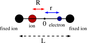
Figure 1: Schematic representation of the model system described by the Hamiltonian (21).

Two ions are fixed at a distance of $L=19.0$ $a_{0}$, the third ion and the electron are free to move in 1D along the line joining the two fixed ions. Here, the symbols $r$ and $R$ are the coordinates of the electron and the movable ion measured from the center of the two fixed ions. The ionic mass is chosen as $M=1836$, the proton mass, whereas the other parameters are tuned in order to make the system essentially a two-electronic-state model. We present here the results obtained by choosing two different sets of parameters, producing strong and weak non-adiabatic couplings, between the first, $\epsilon^{(1)}_{BO}$, and the second BOPES, $\epsilon^{(2)}_{BO}$, around the avoided crossing at $R_{ac}=-1.90$ a₀. The values of the parameters in the Hamiltonian (21) are: $R_{f}=5.0$ a₀, $R_{l}=3.1$ a₀ and $R_{r}=4.0$ a₀, for the strong coupling case; $R_{f}=3.8$ a₀, $R_{l}=2.9$ a₀ and $R_{r}=5.5$ a₀, for the weak coupling case. The BO surfaces are shown in Fig. 2 (upper panels).

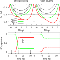
Figure 2: Upper panels: Lowest four BO surfaces, as functions of the nuclear coordinate, for strong (left) and weak (right) non-adiabatic coupling strengths. The first (red line) and second (green line) surfaces correspond to the adiabatic states that are populated during the dynamics, whereas the third and fourth surfaces (dashed black lines) are shown for reference. The squared modulus (reduced by ten times and rigidly shifted in order to superimpose it on the energy curves) of the initial nuclear wave packet is also shown (thin black line). Lower panels: Populations of the two lowest adiabatic states ($\rho_{1}$ and $\rho_{2}$) as functions of time. The arrows represent the time-steps shown in the following figures.

We study the time evolution of this system by choosing the initial wave function as the product of a real-valued normalized Gaussian wave packet, centered at $R_{c}=-4.0$ $a_{0}$ with variance $\sigma=1/\sqrt{2.85}$ $a_{0}$ (thin black line in Fig. 2, upper panels), and the second BO electronic state. To calculate the TDPES, we first solve the TDSE (1) for the complete system, with Hamiltonian (21), and obtain the full wave function, $\Psi(r,R,t)$. This is done by numerical integration of the TDSE using the split-operator-technique Feit et al. (1982), with time-step of $2.4\times 10^{-3}$ fs (or $0.1$ a.u.).

The mean positions and momenta of the FGs evolve along classical trajectories, generated according to Hamilton’s equations

$$\dot{R}_{l}(t)=P_{l}(t)/M;\,\,\dot{P}_{l}(t)=-\partial_{R}\epsilon\left(R,t\right)\big{|}_{R_{l}(t)},$$ (22)

integrated by using the velocity-Verlet algorithm with a time-step of $12.0\times 10^{-3}$ fs (or $0.5$ a.u.). The initial conditions are sampled from the Wigner phase-space distribution corresponding to the initial nuclear wave function. The initial coherent states used in Eq. (15) are thus constructed to determine the (complex-valued) weights $w_{l}$. Numerical results have been obtained for sets of $N_{traj}=2000,5000,10000$ trajectories, with the value  $\gamma=7.0$ a${}_{0}^{-2}$ for the width of the FGs. The coherent states used to represent the nuclear wave function form an overcomplete basis, therefore the sum in Eq. (16) has to be truncated. In order to choose the adequate number of basis functions to include in the sum, energy conservation has been tested and confirmed for all values of $N_{traj}$. The results will be presented only for the case $N_{traj}=5000$. We have computed the RMSD between the exact nuclear density and its approximation in Eq. (16) for a set of values of $\gamma$ and we have chosen the value of this parameter for which the RMSD is minimum (see also the discussion at the end of Section III.1), but clearly other values can be selected.

We will confirm below that the semiclassical FG scheme, adapted to the factorization approach, is an accurate and efficient way to approximate the nuclear wave function. Before presenting the FG results, let us first show different snapshots taken along the dynamics, showing the TDPES. Its feature have been extensively discussed in previous work Abedi et al. (2013a); Agostini et al. (2013, 2014a), but for the sake of completeness, we report here a few configurations. Moreover, we would like to underline that here results for different non-adiabatic coupling strengths will be presented, in order to test the efficiency of the method also in the weak coupling regime.

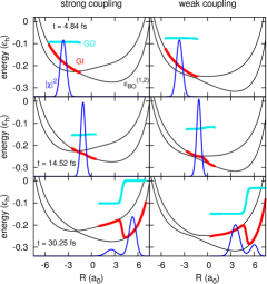
Figure 3: TDPES at different time-steps, as indicated by the arrows in Fig. 2, for strong (left) and weak (right) non-adiabatic coupling strengths. The two lowest BO surfaces (black) are plotted for reference. The GI part of the TDPES (red) presents the well-studied Abedi et al. (2013a); Agostini et al. (2013) dynamical steps that bridge piecewise adiabatic shapes potential energy surface, whereas the GI part Agostini et al. (2014a) (cyan) is piecewise constant. The nuclear density (blue) is shown for reference.

Fig. 3 shows the gauge-invariant (GI) and gauge-dependent (GD) components of the TDPES, namely the two terms that can be identified in Eq. (8) as $\epsilon_{GI}\left({\underline{\underline{\bf R}}},t\right)=\langle\Phi_{\underline{\underline{\bf R}}}(t)|\hat{H}_{el}|\Phi_{\underline{\underline{\bf R}}}(t)\rangle_{\underline{\underline{\bf r}}}$ and $\epsilon_{GD}\left({\underline{\underline{\bf R}}},t\right)=\langle\Phi_{\underline{\underline{\bf R}}}(t)|-i\hbar\partial_{t}|\Phi_{\underline{\underline{\bf R}}}(t)\rangle_{\underline{\underline{\bf r}}}$. The snapshots shown in Fig. 3 are taken along the evolution at the times indicated by the arrows in Fig. 2 (lower panels) and the two lowest adiabatic surfaces are shown for reference. As previously discussed Abedi et al. (2013a); Agostini et al. (2013, 2014a), before the splitting of the nuclear wave packet, the GI part of the TDPES is diabatic, whereas the GD part is constant, and after the splitting the GI component develops steps that bridge between different adiabatic surfaces, whereas the GD part is piecewise constant. The TDPES is only calculated in the regions where the nuclear density is (numerically) not zero. The lack of reliable information beyond the regions shown in the figures is not an issue when classical trajectories or FGs are employed to mimic the nuclear density, as the regions where the exact density is exponentially small are not, or are poorly, sampled.

It is evident from Fig. 3 that we will discuss results for short dynamics, limited to the first half of the oscillation period of the nuclear wave packet in the potential well. Interesting dynamics may arise at later times, when for instance the nuclear wave packet crosses a second time the non-adiabatic coupling region. However, here we focus on the initial non-adiabatic event and test how the FG approximation capture this process. Due to the fact that the analysis reported below is the first attempt to incorporate semiclassically nuclear quantum effects in the exact factorization formalism, we study a simple situation that nonetheless captures the main features of a non-adiabatic event. Also, situations where, for instance, reproducing tunneling dynamics might represent a problem for classically evolving FGs Gelman and Schwartz (2008); Ankerhold (2007); Saltzer and Ankerhold (2003); Kay (2013) will be the subject of further study and not addressed here.

A first set of results is shown in Fig. 4, where we compare the nuclear density, $|\chi(R,t)|^{2}$, from three different calculations: quantum (cyan), employing the full electron-nuclear wave function; classical (green), where the histogram is constructed from the distribution of classical trajectories evolving on the TDPES according to Eqs. (22) (as in Ref. Agostini et al. (2014a)); FG (red), with the nuclear density given in Eq. (16).

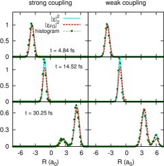
Figure 4: Nuclear density for strong (left) and weak (right) non-adiabatic coupling strengths. Exact results (cyan) are compared with the semiclassical density (red), expressed as sum of FGs, and with the histogram (green) constructed from the distribution of classical positions along the trajectories.

As expected from previous calculations Agostini et al. (2014a), the use of classical trajectories seems to be enough accurate to reproduce the nuclear density. It is however important to stress again, that these results are not obtained by solving a fully approximate form of the coupled electronic and nuclear equations (4) and (5). They only represent a benchmark for any quantum-classical algorithm, since the effect of the electrons, via the TDPES, is treated exactly. The semiclassical density, constructed as the weighted sum of FGs given in Eq. (16), is also accurate. In comparison to the classical histogram, the gain here is the smoothness of the density, not achievable with purely classical trajectories. This feature is extremely important for the calculation of the ENC term containing the gradient of the nuclear density, via the term $-i\hbar\nabla_{\nu}|\chi|/|\chi|$ in Eq. (13).

The second important characteristic of the semiclassical approach is that each FG contributes a phase factor to the full nuclear wave function, thus allowing to determine also the first term on the RHS of Eq. (13). We show this term, i.e. $\nabla_{\nu}S(R,t)$, in Fig. 5, comparing once again exact results with the corresponding FG and classical approximations. The semiclassical value of $\nabla_{\nu}S(R,t)$ is determined as the gradient of the phase in Eq. (17), whereas the function $\nabla_{\nu}S(R,t)$ is classically interpreted as the nuclear momentum evaluated along each trajectory. While the agreement between quantum and FG results is remarkable, the phase-space points corresponding to the classical trajectories do not allow to reconstruct a smooth function of $R$. Even if the number of classical trajectories is increased, the phase-space points are too “noisy” to allow for reconstructing a smooth function. A smoothing algorithm should then be employed, but the numerical efficiency of the whole procedure might become questionable.

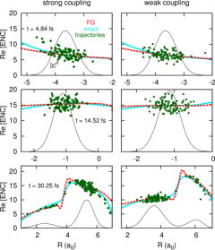
Figure 5: Real part of the ENC term for strong (left) and weak (right) non-adiabatic coupling strengths. The nuclear density (black) is shown for reference. Exact results (cyan) are compared with semiclassical calculations (red) and with the classical phase-space points (green).

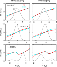
Figure 6: Imaginary part of the ENC term for strong (left) and weak (right) non-adiabatic coupling strengths. The color code is the same as in Fig. 5.

Fig. 6 shows the imaginary part of the ENC term from Eq. (13) at different time-steps during the dynamics, as in previous figures. The exact results (cyan) are compared only with the approximation (red) based on the semiclassical propagation of FGs. Even if we employ a simplified form of the Herman-Kluk propagator, where the pre-factor is set to 1, semiclassical results are in satisfactory good agreement with exact results.

One could consider improving the approach developed here by, for instance, explicitly computing the Herman-Kluk pre-factor, at the expenses of increasing the computational cost.

V Conclusion

We have reported our first semiclassical procedure adapted to the formalism of the exact factorization of the electron-nuclear wave function Abedi et al. (2010, 2012). The approach has been used to estimate the ENC term that explicitly depends on the nuclear wave function (gradient of its modulus and phase) in the electronic equation. In previous work Abedi et al. (2014); Agostini et al. (2014b) on the development of a mixed quantum-classical algorithm in the context of the exact factorization, such term has been treated fully classically and identified as the nuclear momentum. However, we observed that, despite the fact that this approximation is widely used in the literature Tully (1990); Jasper et al. (2004); Nielsen et al. (2000), correction terms naturally arise in the factorization framework. The extent and role of the corrections may depend on the process that we intend to study, therefore we have shown in the present paper how to evaluate such corrections based on the semiclassical propagation of FGs, for a simple model case of non-adiabatic charge transfer. The main gain in using FGs, rather than a purely classical approach, lies in the possibility of obtaining smooth functions whose gradients can be easily determined without introducing large numerical errors.

The semiclassical results shown in the paper have been obtained by evolving FGs on the exact TDPES, that is known for the simple model system studied here as the outcome of exact calculations based on the numerical solution of the full TDSE. This procedure is a test, since the only approximation is the semiclassical treatment of the nuclear dynamics, whereas the electrons are treated exactly, via the information encoded in the TDPES. Moreover, this study provides a benchmark for future development, aiming at improving the initial, and lowest-order, mixed quantum-classical algorithm derived from the factorization Abedi et al. (2014); Agostini et al. (2014b). The procedure described here can be easily implemented in an algorithm, as we will present elsewhere Min et al. (tted), resulting in a novel mixed quantum-semiclassical scheme for solving coupled electron-nuclear dynamics.

References

- Polli et al. (2010) D. Polli, P. Altoè, O. Weingart, K. M. Spillane, C. Manzoni, D. Brida, G. Tomasello, G. Orlandi, P. Kukura, R. A. Mathies, M. Garavelli, and G. Cerullo, Nature 467, 440 (2010).
- Chung et al. (2012) W. C. Chung, S. Nanbu, and T. Ishida, J. Phys. Chem. B 116, 8009 (2012).
- Rozzi et al. (2013) C. A. Rozzi, S. M. Falke, N. Spallanzani, A. Rubio, E. Molinari, D. Brida, M. Maiuri, G. Cerullo, H. Schramm, J. Christoffers, and C. Lienau, Nat. Communic. 4, 1602 (2013).
- Jailaubekov et al. (2013) A. E. Jailaubekov, A. P. Willard, J. R. Tritsch, W.-L. Chan, N. Sai, R. Gearba, L. G. Kaake, K. J. Williams, K. Leung, P. J. Rossky, and X.-Y. Zhu, Nat. Mater. 12, 66 (2013).
- McEniry et al. (2007) E. J. McEniry, D. R. Bowler, D. Dundas, A. P. Horsfield, C. G. Sánchez, and T. N. Todorov, J. Phys.: Condens. Matter 19, 196201 (2007).
- Horsfield et al. (2004) A. P. Horsfield, D. R. Bowler, A. J. Fisher, and T. N. Todorov, J. Phys.: Condens. Matter 16, 3609 (2004).
- Meyer et al. (1990) H.-D. Meyer, U. Manthe, and L. S. Cederbaum, Chem. Phys. Lett. 165, 73 (1990).
- Manthe et al. (1992) U. Manthe, H.-D. Meyer, and L. S. Cederbaum, J. Chem. Phys. 97, 3199 (1992).
- Burghardt et al. (1999) I. Burghardt, H.-D. Meyer, and L. S. Cederbaum, J. Chem. Phys. 111, 2927 (1999).
- Meyer and Worth (2003) H.-D. Meyer and G. A. Worth, Theor. Chim. Acta 109, 251 (2003).
- Thoss et al. (2004) M. Thoss, W. Domcke, and H. Wang, Chem. Phys. 296, 217 (2004).
- L. Wang and May (2003) H.-D. M. L. Wang and V. May, J. Chem. Phys. 125, 014102 (2003).
- Westermann et al. (2011) T. Westermann, R. Brodbeck, W. S. Alexander B. Rozhenko and, and U. Manthe, J. Chem. Phys. 135, 184102 (2011).
- Wang and Thoss (2003) H. Wang and M. Thoss, J. Chem. Phys. 119, 1289 (2003).
- Li et al. (2010) J. Li, I. Kondov, H. Wang, and M. Thoss, J. Phys. Chem. C 114, 18481 (2010).
- Meng et al. (2012) Q. Meng, S. Faraji, O. Vendrell, and H.-D. Meyer, J. Chem. Phys. 137, 134302 (2012).
- Schröder et al. (2008) M. Schröder, J.-L. C. n Macedo, and A. Brown*, Phys. Chem. Chem. Phys. 10, 850 (2008).
- Martínez and Levine (1996) T. J. Martínez and R. D. Levine, Chem. Phys. Lett. 259, 252 (1996).
- Martínez et al. (1996) T. J. Martínez, M. Ben-Nun, and R. D. Levine, J. Phys. Chem. 100, 7884 (1996).
- Martìnez (2006) T. J. Martìnez, Acc. Chem. Res. 39, 119 (2006).
- Ehrenfest (1927) P. Ehrenfest, Zeitschrift für Physik 45, 455 (1927).
- Pechukas (1969) P. Pechukas, Phys. Rev. 181, 174 (1969).
- Tully (1990) J. C. Tully, J. Chem. Phys. 93, 1061 (1990).
- Stock and Thoss (1997) G. Stock and M. Thoss, Phys. Rev. Lett. 78, 578 (1997).
- Sun and Miller (1997) X. Sun and W. H. Miller, J. Chem. Phys. 106, 6346 (1997).
- Jasper et al. (2004) A. W. Jasper, C. Zhu, S. Nangia, and D. G. Truhlar, Faraday Discuss. 127, 1 (2004).
- Nielsen et al. (2000) S. Nielsen, R. Kapral, and G. Ciccotti, J. Chem. Phys. 112, 6543 (2000).
- Hsieh and Kapral (2013) C.-Y. Hsieh and R. Kapral, J. Chem. Phys. 138, 134110 (2013).
- Bonella and Coker (2005) S. Bonella and D. F. Coker, J. Chem. Phys. 122, 194102 (2005).
- Huo and Coker (2012) P. Huo and D. F. Coker, J. Chem. Phys. 137, 22A535 (2012).
- Doltsinis and Marx (2002) N. L. Doltsinis and D. Marx, Phys. Rev. lett. 88, 166402 (2002).
- Curchod et al. (2011) B. F. E. Curchod, I. Tavernelli, and U. Rothlisberger, Phys. Chem. Chem. Phys. 13, 3231 (2011).
- Wyatt et al. (2001) R. E. Wyatt, C. L. Lopreore, and G. Parlant, J. Chem. Phys. 114, 5113 (2001).
- Burghardt (2005) I. Burghardt, J. Chem. Phys. 122, 094103 (2005).
- Prezhdo and Brooksby (2001) O. V. Prezhdo and C. Brooksby, Phys. Rev. Lett. 86, 3215 (2001).
- Zamstein and Tannor (2012) N. Zamstein and D. J. Tannor, J. Chem. Phys. 137, 22A518 (2012).
- Bousquet et al. (2011) D. Bousquet, K. H. Hughes, D. A. Micha, and I. Burghardt, J. Chem. Phys. 134, 064116 (2011).
- Richardson and Thoss (2013) J. O. Richardson and M. Thoss, J. Chem. Phys. 139, 031102 (2013).
- Ananth (2013) N. Ananth, J. Chem. Phys. 139, 124102 (2013).
- Abedi et al. (2010) A. Abedi, N. T. Maitra, and E. K. U. Gross, Phys. Rev. Lett. 105, 123002 (2010).
- Abedi et al. (2012) A. Abedi, N. T. Maitra, and E. K. U. Gross, J. Chem. Phys. 137, 22A530 (2012).
- Abedi et al. (2013a) A. Abedi, F. Agostini, Y. Suzuki, and E. K. U. Gross, Phys. Rev. Lett 110, 263001 (2013a).
- Agostini et al. (2013) F. Agostini, A. Abedi, Y. Suzuki, and E. K. U. Gross, Mol. Phys. 111, 3625 (2013).
- Agostini et al. (2014a) F. Agostini, A. Abedi, Y. Suzuki, S. K. Min, N. T. Maitra, and E. K. U. Gross, arXiv:1406.4667 [physics.chem-ph] (2014a).
- Abedi et al. (2014) A. Abedi, F. Agostini, and E. K. U. Gross, Europhys. Lett. 106, 33001 (2014).
- Agostini et al. (2014b) F. Agostini, A. Abedi, and E. K. U. Gross, J. Chem. Phys. 141, 214101 (2014b).
- Vleck (1928) J. H. V. Vleck, Proc. Nat. Ac. Sci. 14, 178 (1928).
- Min et al. (tted) S. K. Min, F. Agostini, and E. K. U. Gross, (to be submitted).
- Heller (1981) E. J. Heller, J. Chem. Phys. 75, 2923 (1981).
- Herman and Kluk (1984) M. F. Herman and E. Kluk, Chem. Phys. 91, 27 (1984).
- Kluk et al. (1986) E. Kluk, M. F. Herman, and H. L. Davis, J. Chem. Phys. 84, 326 (1986).
- Kay (2006) K. G. Kay, Chem. Phys. 322, 3 (2006).
- Miller (2002) W. H. Miller, Mol. Phys. 100, 397 (2002).
- Miller (1970) W. H. Miller, J. Chem. Phys. 53, 3578 (1970).
- Thoss and Wang (2004) M. Thoss and H. Wang, Ann. Rev. Phys. Chem. 55, 299 (2004).
- Kay (2005) K. G. Kay, Ann. Rev. Phys. Chem. 56, 255 (2005).
- Miller (2001) W. H. Miller, J. Phys. Chem A 105, 2942 (2001).
- Shin and Metiu (1995) S. Shin and H. Metiu, J. Chem. Phys. 102, 23 (1995).
- Hunter (1975) G. Hunter, Int. J. Quantum Chem 9, 237 (1975).
- Gidopoulos and Gross (2014) N. I. Gidopoulos and E. K. U. Gross, Phil. Trans. R. Soc. A 372, 20130059 (2014).
- Frenkel (1934) J. Frenkel, Wave mechanics, Clarendon, Oxford ed. (1934).
- McLachlan (1964) A. D. McLachlan, Mol. Phys. 8, 39 (1964).
- Alonso et al. (2013) J. L. Alonso, J. Clemente-Gallardo, P. Echeniche-Robba, and J. A. Jover-Galtier, J. Chem. Phys. 139, 087101 (2013).
- Abedi et al. (2013b) A. Abedi, N. T. Maitra, and E. K. U. Gross, J. Chem. Phys. 139, 087102 (2013b).
- Ghosh and Dhara (1988) S. K. Ghosh and A. K. Dhara, Phys. Rev. A 38, 1149 (1988).
- Runge and Gross (1984) E. Runge and E. K. U. Gross, Phys. Rev. Lett. 52, 997 (1984).
- Min et al. (2014) S. K. Min, A. Abedi, K. S. Kim, and E. K. U. Gross, Phys. Rev. Lett. 113, 263004 (2014).
- Note (1) To be precise, the nuclear density is approximated, within the classical treatment, as -function, centered at all times at the classical trajectory. But this contribution is totally omitted in the expression of the ENC term.
- Feit et al. (1982) M. D. Feit, F. A. Fleck Jr., and A. Steiger, J. Comput. Phys. 47, 412 (1982).
- Note (2) The value of is chosen to have the best overlap between the initial semiclassical density and the exact density, in order to impose initial conditions as close as possible to the exact ones.
- Gelman and Schwartz (2008) D. Gelman and S. D. Schwartz, J. Chem. Phys. 129, 024504 (2008).
- Ankerhold (2007) J. Ankerhold, Quantum tunnelling in complex systems. The semiclassical approach, Springer Tracts in Modern Physics, Vol. 224 (Springer-Verlag Berlin Heidelberg, 2007).
- Saltzer and Ankerhold (2003) M. Saltzer and J. Ankerhold, Phys. Rev. A 68, 042108 (2003).
- Kay (2013) K. G. Kay, Phys. Rev. A 88, 012122 (2013).