SISSA 03/2015/FISI

TTP15-003

Leptogenesis in an SU(5)$\,\times\,$A₅
Golden Ratio Flavour Model

Julia Gehrlein${}^{\,a,}$ , Serguey T. Petcov${}^{\,b,c,}$ , Martin Spinrath${}^{\,a,}$ , Xinyi Zhang${}^{\,d,}$

^a Institut für Theoretische Teilchenphysik, Karlsruhe Institute of Technology,

Engesserstraße 7, D-76131 Karlsruhe, Germany

^b SISSA/INFN, Via Bonomea 265, I-34136 Trieste, Italy

^c Kavli IPMU (WPI), University of Tokyo, Tokyo, Japan

^d School of Physics and State Key Laboratory of Nuclear Physics and Technology,

Peking University, 100871 Beijing, China

In this paper we discuss a minor modification of a previous SU(5)$\,\times\,$A₅ flavour model which exhibits at leading order golden ratio mixing and sum rules for the heavy and the light neutrino masses. Although this model could predict all mixing angles well it fails in generating a sufficient large baryon asymmetry via the leptogenesis mechanism. We repair this deficit here, discuss model building aspects and give analytical estimates for the generated baryon asymmetry before we perform a numerical parameter scan. Our setup has only a few parameters in the lepton sector. This leads to specific constraints and correlations between the neutrino observables. For instance, we find that in the model considered only the neutrino mass spectrum with normal mass ordering and values of the lightest neutrino mass in the interval $10-18$ meV are compatible with the current data on the neutrino oscillation parameters. With the introduction of only one NLO operator, the model can accommodate successfully simultaneously even at $1\sigma$ level the current data on neutrino masses, on neutrino mixing and the observed value of the baryon asymmetry.

1 Introduction

The theoretical explanation for the observed neutrino oscillations and neutrino masses requires physics beyond the Standard Model. Furthermore the presence of Dark Matter and the observed baryon asymmetry of the Universe (BAU) support the need for a more fundamental theory. In the present article we will establish a connection between two of the above mentioned observations and investigate the Baryogenesis through leptogenesis scenario [1] in an $\text{SU}(5)\times\text{A}_{5}$ flavour model. The model we are going to discuss here is the first GUT A₅ golden ratio flavour model with successful leptogenesis to our knowledge. This recently proposed model [2] has the feature that $\theta_{12}$ is connected to the golden ratio $\phi_{g}=\frac{1+\sqrt{5}}{2}$ via $\theta_{12}=\tan^{-1}\left(\frac{1}{\phi_{g}}\right)$. Similar to the golden ratio (GR) type A models in [3] the reactor angle is predicted to be vanishing at leading order and the atmospheric angle to be maximal. Hence, the neutrino mixing matrix $U_{\text{GR}}$ has the form

$$U_{\text{GR}}=\begin{pmatrix}\sqrt{\frac{\phi_{g}}{\sqrt{5}}}&\sqrt{\frac{1}{\phi_{g}\sqrt{5}}}&0\\ -\sqrt{\frac{1}{2\phi_{g}\sqrt{5}}}&\sqrt{\frac{\phi_{g}}{2\sqrt{5}}}&\frac{1}{\sqrt{2}}\\ \sqrt{\frac{1}{2\phi_{g}\sqrt{5}}}&-\sqrt{\frac{\phi_{g}}{2\sqrt{5}}}&\frac{1}{\sqrt{2}}\end{pmatrix}P_{0}\;,$$ (1.1)

which is given in the convention of the Particle Data Group [4] with the diagonal matrix $P_{0}$ = Diag$(\text{exp}(-\tfrac{\text{i}\alpha_{1}}{2}),\text{exp}(-\tfrac{\text{i}\alpha_{2}}{2}),1)$ containing the Majorana phases. Since the experimental values for the angles, cf. Tab. 1, strongly disfavour $\theta_{13}$ to be vanishing the leading order mixing angles have to be corrected to realistic values. In [2] we followed the approach based on Grand Unification where the neutrino mixing angles receive corrections from the charged lepton sector. Namely this model features SU(5) unification. Thereby we could explore the SU(5) relation $\theta_{13}\approx\theta_{C}/\sqrt{2}$ from the non-standard Yukawa-coupling relations $y_{\tau}/y_{b}=-1.5$ and $y_{\mu}/y_{s}=6$ [6, 7], and for the double ratio $(y_{\mu}/y_{s})(y_{d}/y_{e})=12$ which are all in perfect agreement with experimental data.

In addition to the corrections from the charged lepton sector renormalisation group running effects (RGE) have to be taken into account. Due to a neutrino mass sum rule in both hierarchies only a certain mass range is allowed. For the inverted ordering this implies large RGE effects for $\theta_{12}$ which rule out this ordering.

Since the light neutrino masses are generated via the type-I-seesaw mechanism in [2] the Baryogenesis through leptogenesis mechanism can be easily implemented. In this mechanism the dynamically generated lepton asymmetry is converted into a baryon asymmetry due to sphaleron interactions. Thermal leptogenesis can take place when the heavy RH Majorana neutrinos (and their SUSY partners the sneutrinos) decay out-of-equilibrium in a CP and lepton-number violating way. Flavour effects [8, 9, 10] (see also, e.g., [11, 12, 13, 14]) can play an important role in thermal leptogenesis. We set the scale at which leptogenesis takes place to be the see-saw scale $M_{S}=10^{13}$ GeV. In the model considered we have also $\tan\beta=30$ [2], and thus, the scale $M_{S}$ falls in the interval $10^{9}(1+\tan^{2}\beta)$ GeV$<M_{S}<10^{12}(1+\tan^{2}\beta)$ GeV. For values of $M_{S}$ in this interval [15] the baryon asymmetry is produced in the two-flavour leptogenesis regime and we perform the analysis of baryon asymmetry generation in this regime.

We will see that the original model cannot accommodate for the observed value of the baryon asymmetry due to the structure of the neutrino Yukawa matrix. In fact, there would be no baryon asymmetry generated via the leptogenesis mechanism. In order to generate a non-zero asymmetry we will introduce only one additional operator in the neutrino sector which corrects the neutrino Yukawa matrix and subsequently affects the phenomenology of the model.

The paper is organized as follows: Section 2 is a short overview of the model building aspects including the NLO operator. In section 3 we discuss the analytical results for the phenomenology of the model. There we also describe the relevant formulas for leptogenesis. In section 4 we show the results of a numerical parameter scan. We discuss the predictions for the mixing parameters including the phases as well as for the sum of the neutrino masses, the observable in neutrinoless double beta-decay, the kinematic mass $m_{\beta}$ and for the generated baryon asymmetry. In section 5 we summarise and conclude.

Parameter	best-fit ($\pm 1\sigma$)	$3\sigma$ range
$\theta_{12}$ in ∘	$33.48^{+0.78}_{-0.75}$	$31.29\rightarrow 35.91$
$\theta_{13}$ in ∘	$8.50^{+0.20}_{-0.21}$	$7.85\rightarrow 9.10$
$\theta_{23}$ in ∘	$42.3^{+3.0}_{-1.6}$	$38.2\rightarrow 53.3$
$\delta$ in ∘	$306^{+39}_{-70}$	$0\rightarrow 360$
$\Delta m_{21}^{2}$ in $10^{-5}$ eV2	$7.50^{+0.19}_{-0.17}$	$7.02\rightarrow 8.09$
$\Delta m_{31}^{2}$ in $10^{-3}$ eV2	$2.457^{+0.047}_{-0.047}$	$2.317\rightarrow 2.607$

Table 1: The best-fit values and the 3$\sigma$ ranges for the parameters in the normal ordering taken from [5].

2 Model building aspects

The model we are going to discuss is based on the SU(5)$\times$A₅ model proposed in [2]. We only had to extend it minimally to accommodate successful leptogenesis. The modification we are going to introduce has further implications for the phenomenology. We focus first on the related model building aspects. We briefly revise the leading order (LO) superpotential for the neutrino sector, which is identical to the original model before we introduce the corrections. They are induced by an additional operator in the superpotential which yields next-to-leading order (NLO) corrections to the Yukawa couplings while the right-handed neutrino Majorana mass matrix remains unaffected. This single higher order operator will generate a sufficiently large baryon asymmetry to be in agreement with the experimental observations.

2.1 The neutrino sector at LO

We briefly summarise next the relevant parts of the original SU(5)$\times$A₅ model from [2]. We are not going to discuss the flavon vacuum alignment which does not change at all and is given in the original paper.

The matter content of our model is organised in ten-dimensional representations of SU(5), $T_{i}$ with $i=1$, 2, 3, five-dimensional representations $F$, and one-dimensional representations $N$ which transform as one-, three- and three-dimensional representations of A₅ respectively, see also Tab. 2.

Additionally, we had introduced in the original model the following flavons which will appear in the neutrino sector. There are two flavons which transform as one-dimensional representations under A₅

$$\langle\theta_{2}\rangle=v_{\theta_{2}}\;,\quad\langle\epsilon_{1}\rangle=v_{\epsilon_{1}}\;,$$ (2.1)

one flavon in a three-dimensional representation

$$\langle\phi_{3}\rangle=v_{\phi}^{(3)}\left(0,0,1\right)\;,$$ (2.2)

and one flavon in a five-dimensional representation

$$\langle\omega\rangle=\left(\sqrt{\tfrac{2}{3}}(v_{2}+v_{3}),v_{3},v_{2},v_{2},v_{3}\right)\;.$$ (2.3)

Their charges under the shaping symmetries are given in Tab. 2. Note especially that no new flavon appeared.

	$\mathrm{SU(5)}$	$\mathrm{A_{5}}$	$\mathbb{Z}_{4}^{R}$	$\mathbb{Z}_{2}$	$\mathbb{Z}_{2}$	$\mathbb{Z}_{3}$	$\mathbb{Z}_{3}$	$\mathbb{Z}_{3}$	$\mathbb{Z}_{3}$	$\mathbb{Z}_{3}$	$\mathbb{Z}_{3}$	$\mathbb{Z}_{4}$
$F$	$\mathbf{\bar{5}}$	$\mathbf{3}$	$1$	$0$	$0$	$0$	$0$	$1$	$2$	$0$	$0$	$0$
$N$	$\mathbf{1}$	$\mathbf{3}$	$1$	$0$	$0$	$0$	$0$	$0$	$2$	$0$	$0$	$2$
$T_{1}$	$\mathbf{10}$	$\mathbf{1}$	$1$	$1$	$0$	$2$	$2$	$2$	$2$	$0$	$0$	$0$
$T_{2}$	$\mathbf{10}$	$\mathbf{1}$	$1$	$0$	$0$	$0$	$2$	$1$	$1$	$0$	$0$	$3$
$T_{3}$	$\mathbf{10}$	$\mathbf{1}$	$1$	$0$	$0$	$0$	$0$	$2$	$2$	$0$	$0$	$3$
$H_{5}$	$\mathbf{5}$	$\mathbf{1}$	$0$	$0$	$0$	$0$	$0$	$2$	$2$	$0$	$0$	$2$
$\bar{H}_{5}$	$\mathbf{\bar{5}}$	$\mathbf{1}$	$0$	$0$	$0$	$2$	$1$	$2$	$0$	$0$	$1$	$0$
$\phi_{3}$	$\mathbf{1}$	$\mathbf{3}$	$0$	$1$	$1$	$0$	$2$	$0$	$2$	$2$	$0$	$1$
$\omega$	$\mathbf{1}$	$\mathbf{5}$	$0$	$0$	$0$	$0$	$0$	$0$	$2$	$0$	$0$	$0$
$\theta_{2}$	$\mathbf{1}$	$\mathbf{1}$	$0$	$1$	$1$	$0$	$2$	$1$	$2$	$1$	$0$	$3$
$\epsilon_{1}$	$\mathbf{1}$	$\mathbf{1}$	$0$	$0$	$0$	$0$	$1$	$1$	$1$	$0$	$0$	$0$
$\Gamma_{1}$	$\mathbf{1}$	$\mathbf{3}$	$0$	$0$	$0$	$0$	$1$	$1$	$1$	$0$	$0$	$0$
$\bar{\Gamma}_{1}$	$\mathbf{1}$	$\mathbf{3}$	$2$	$0$	$0$	$0$	$2$	$2$	$2$	$0$	$0$	$0$
$\Gamma_{3}$	$\mathbf{1}$	$\mathbf{1}$	$0$	$0$	$0$	$0$	$2$	$2$	$2$	$0$	$0$	$0$
$\bar{\Gamma}_{3}$	$\mathbf{1}$	$\mathbf{1}$	$2$	$0$	$0$	$0$	$1$	$1$	$1$	$0$	$0$	$0$
$\Psi_{1}$	$\mathbf{5}$	$\mathbf{3}$	$1$	$0$	$0$	$0$	$1$	$0$	$2$	$0$	$0$	$0$
$\bar{\Psi}_{1}$	$\mathbf{\bar{5}}$	$\mathbf{3}$	$1$	$0$	$0$	$0$	$2$	$0$	$1$	$0$	$0$	$0$
$\Psi_{2}$	$\mathbf{5}$	$\mathbf{3}$	$0$	$0$	$0$	$0$	$1$	$0$	$0$	$0$	$0$	$2$
$\bar{\Psi}_{2}$	$\mathbf{\bar{5}}$	$\mathbf{3}$	$2$	$0$	$0$	$0$	$2$	$0$	$0$	$0$	$0$	$2$

Table 2: Charges under $\mathbb{Z}_{n}$ and $\mathrm{SU(5)}$ and $\mathrm{A_{5}}$ representations of all the fields appearing in the neutrino sector of the model. Note that the only new fields compared to [2] are the messenger fields $\Psi_{1}$, $\bar{\Psi}_{1}$, $\Psi_{2}$ and $\bar{\Psi}_{2}$.

We are not going to discuss here the quark sector, it was analysed in [2]. In what concerns the charged lepton sector, we only note that for the matrix of charged lepton Yukawa couplings we find

$$Y_{e} =\begin{pmatrix}0&-1/2a_{21}&0\\ 6a_{12}&6a_{22}&6a_{32}\\ 0&0&-3/2a_{33}\\ \end{pmatrix}~{}\;.$$ (2.4)

The order one coefficients in front of the parameters $a_{ij}$ are SU(5) Clebsch-Gordan coefficients which imply that

$$\theta_{13}\approx\frac{1}{\sqrt{2}}\theta_{C}\;,$$ (2.5)

where $\theta_{C}$ is the Cabibbo angle. This is only possible due to the non-standard Clebsch-Gordan coeffcients [6] as it was realised in a series of papers [7].

The flavon $\omega$ is responsible for the GR structure of the Majorana mass matrix which can be seen in the LO superpotential for the neutrino sector which reads

$$\mathcal{W}^{\text{LO}}_{\nu} =y_{1}^{n}FNH_{5}+y_{2}^{n}NN\omega\;.$$ (2.6)

The right-handed neutrino mass matrix then reads

$$M_{\text{RR}} =y_{2}^{n}\begin{pmatrix}2\sqrt{\frac{2}{3}}(v_{2}+v_{3})&-\sqrt{3}v_{2}&-\sqrt{3}v_{2}\\ -\sqrt{3}v_{2}&\sqrt{6}v_{3}&-\sqrt{\frac{2}{3}}(v_{2}+v_{3})\\ -\sqrt{3}v_{2}&-\sqrt{\frac{2}{3}}(v_{2}+v_{3})&\sqrt{6}v_{3}\\ \end{pmatrix}\;$$ (2.7)

and the neutrino Yukawa couplings are

$$Y_{\nu}^{\text{LO}}=y_{1}^{n}\begin{pmatrix}1&0&0\\ 0&0&1\\ 0&1&0\end{pmatrix}\;,$$ (2.8)

which are diagonalised by the golden ratio mixing matrix $U_{\text{GR}}$ from eq. (1.1). Note that we are using the right-left convention for the Yukawa matrices, which means that the first index of the matrix corresponds to the SU(2)_L singlet.

This is the structure of the original model which cannot accommodate for the observed value of the baryon asymmetry of the universe, as we will see later on. In order to generate a non-zero asymmetry we follow the approach as described in [16] and introduce an additional operator which perturbs the original flavour structure of the model. Note nevertheless, that compared to [16] we do not introduce an additional flavon and no additional shaping symmetries. Here it is sufficient to extend minimally the messenger content of the model.

2.2 The neutrino sector at NLO

In this section we discuss the NLO superpotential of the neutrino sector. In order to accommodate leptogenesis which can generate the observed value of the baryon asymmetry, we will introduce a correction to the neutrino Yukawa matrix governed by the operator $FN\phi_{3}\theta_{2}H_{5}\epsilon_{1}^{2}$. This operator was absent in the original model but can be added by introducing only two new pairs of messenger fields $\Psi_{1}$, $\bar{\Psi}_{1}$, $\Psi_{2}$ and $\bar{\Psi}_{2}$.

The renormalisable superpotential of the NLO neutrino sector reads

$$\begin{split}\mathcal{W}_{\nu}^{\text{ren, NLO}}&=M_{\Psi_{1}}\Psi_{1}\bar{\Psi}_{1}+M_{\Psi_{2}}\Psi_{2}\bar{\Psi}_{2}+F\Psi_{1}\Gamma_{3}+N\bar{\Psi}_{1}\Psi_{2}+\bar{\Psi}_{2}H_{5}\Gamma_{1}+\epsilon_{1}\epsilon_{1}\bar{\Gamma}_{3}+\theta_{2}\phi_{3}\bar{\Gamma}_{1}\;,\end{split}$$ (2.9)

where we have omitted the coupling constants to increase clarity and only write down the operators which are new. We assume the messenger masses to be larger than the GUT scale and to be related to the messenger scale $\Lambda$ by $\mathcal{O}(1)$ coefficients. The charges of the new messenger fields under the $\mathbb{Z}_{n}$ symmetries as well as their SU(5) and A₅ representations are shown in Tab. 2. The corresponding supergraphs for the leading order operator and the next-to-leading order operator for the neutrino Yukawa matrix can be found in Fig. 1.

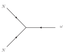
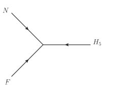
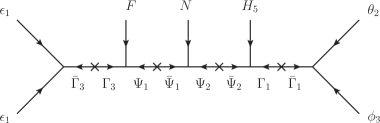
Figure 1: The supergraphs for the neutrino sector including LO and NLO operators.

No new operators compared to the original model are possible apart from the one we discuss now. The only new effective operator is

$$\mathcal{W}_{\nu}^{\text{NLO}}=\frac{1}{\Lambda^{4}}((NF)_{\bf 3}\phi_{3})_{\bf 1}H_{5}\theta_{2}\epsilon_{1}^{2}\;,$$ (2.10)

where we have denoted with brackets the A₅ contractions. This operator gives a correction to the neutrino Yukawa matrix

$$\delta Y_{\nu}\equiv|y_{1}^{n}|c\text{ e}^{\text{i }\gamma}\begin{pmatrix}0&1&0\\ -1&0&0\\ 0&0&0\\ \end{pmatrix}\;,$$ (2.11)

where $0<c\ll 1$. This correction disturbs the golden ratio mixing pattern already in the neutrino sector by itself and subsequently the phenomenology of the original model, especially the prediction for leptogenesis is modified.

3 Phenomenology: Analytical Results

In this section we will discuss the phenomenological implications of introducing $\delta Y_{\nu}$. Because $c$ is small, in many cases the results are similar to those obtained in the original model. However, as we will see, in some cases when the leading order result was relatively small, a correction of order $c$ can have a sizeable impact.

3.1 Masses and Mixing Angles

The original model was very predictive due to the built-in sum rules. And indeed one mass sum rule remains valid. Since $M_{\text{RR}}$ is not corrected the sum rule for the right-handed neutrino masses

$$M_{1}+M_{2}=M_{3}\;,$$ (3.1)

is still correct. Note that, the masses are taken here to be complex.

The situation for the light neutrino masses is somewhat different: they get corrections of the order of $c^{2}\ll 1$. However, since these corrections are small, the sum rule

$$\frac{\text{e}^{\text{i}\,\alpha_{1}}}{\left|m_{1}\right|}+\frac{\text{e}^{\text{i}\,\alpha_{2}}}{\left|m_{2}\right|}-\frac{1}{\left|m_{3}\right|}=\mathcal{O}(c^{2})\approx 0$$ (3.2)

is still a good approximation. And hence our estimate for the ranges of the neutrino masses from [2]

$$0.011\text{ eV} \lesssim m_{1}\phantom{\lesssim 0.454\text{ eV}}\text{ for NO,}$$ (3.3)

$$0.028\text{ eV} \lesssim m_{3}\lesssim 0.454\text{ eV}\text{ for IO.}$$ (3.4)

is still reasonable. For all three PMNS mixing angles we find corrections of order $c$. For $\theta_{13}$ and $\theta_{23}$ the expressions are somewhat lengthy and not insightful, but as an example we find as correction for $\theta_{12}$ to first order in $c$

$$\delta\theta_{12}^{\nu} =-\frac{c\cos\gamma}{\sqrt{2}}-\frac{\sqrt{2}c\Im(M_{1}^{\star}M_{2})\sin\gamma}{|M_{1}^{2}|-|M_{2}^{2}|}\;.$$ (3.5)

The corrections have immediate consequences for the phenomenology.

The first thing one might wonder, is if the inverted mass ordering is still excluded like in the original model. We begin our discussion with the sum rule [17]

$$\sin^{2}\theta_{12}=\cos^{2}\theta^{\nu}_{12}+\frac{\sin 2\theta_{12}\sin\theta_{13}\cos\delta-\tan\theta_{23}\cos 2\theta^{\nu}_{12}}{\tan\theta_{23}(1-\cot^{2}\theta_{23}\,\sin^{2}\theta_{13})}\,,$$ (3.6)

where $\cos^{2}\theta^{\nu}_{12}=\phi_{g}/\sqrt{5}$ and $\cos 2\theta^{\nu}_{12}=2\phi_{g}/\sqrt{5}-1$.

For $c=0$ we can evaluate this sum rule and find $\theta_{12}\gtrsim 23^{\circ}$ (compared to $\theta_{12}\gtrsim 24^{\circ}$ from the sum rule in [18]). Using the lower bound on the mass scale in the inverted ordering case, cf. eq. (3.4), we can estimate that the RGE evolved value of $\theta_{12}$ at the seesaw scale has to be smaller than about 5.7^∘. Attributing this difference completely to the correction $\delta\theta_{12}^{\nu}$ with $\gamma=0$ or $\pi$ we find $c\gtrsim 0.43$. This is a crude estimate because the other mixing angles are affected as well modifying the above sum rule in a non-trivial way. Nevertheless, from here we would still expect $c$ to be of order $0.1$ to safe the inverted mass ordering. On the other hand such a large value for $c$ is not plausible from a model building point of view because it is associated to a highly suppressed operator making values of $c=10^{-4}$ to $10^{-3}$ plausible. We will come back to this point later when we discuss the numerical results.

For future convenience, we introduce the following definitions for the parameters which we will use as well in our numerical scan

$$M_{1} =\frac{1}{\sqrt{6}}(X+Y)=\frac{1}{\sqrt{6}}|X||1+\rho\text{ e}^{\text{i}\phi}|\text{e}^{\text{i}\phi_{1}},~{}\phi_{1}=\text{arg}(X+Y)~{},$$ (3.7)

$$M_{2} =\frac{1}{\sqrt{6}}(X-Y)=\frac{1}{\sqrt{6}}|X||1-\rho\text{ e}^{\text{i}\phi}|\text{e}^{\text{i}\phi_{2}},~{}\phi_{2}=\text{arg}(X-Y)~{},$$ (3.8)

$$M_{3} =\sqrt{\frac{2}{3}}X=\sqrt{\frac{2}{3}}|X|\text{ e}^{\text{i}\phi_{3}},~{}\phi_{3}=\text{arg}(X)~{},$$ (3.9)

where

$$X =(4v_{3}+v_{2})y_{2}^{n}~{},$$ (3.10)

$$Y =3\sqrt{5}v_{2}y_{2}^{n}~{},$$ (3.11)

$$\rho =\left|\frac{Y}{X}\right|~{},$$ (3.12)

$$\phi =\text{arg}(Y)-\text{arg}(X)~{}.$$ (3.13)

In this way, we express the absolute value of the three heavy neutrino masses in terms of three real parameters, i.e., $|X|$, $\rho$ and $\phi$. $|X|$ sets the scale of our interest. $\rho$ reflects the detailed structure of the heavy neutrino mass spectrum. $\phi$ is connected to $\rho$ via the ratio of two mass squared differences

$$\frac{\Delta m_{21}^{2}}{\Delta m_{31}^{2}}=\frac{16\rho\cos\phi}{(\rho^{2}-2\rho\cos\phi+1)(\rho^{2}+2\rho\cos\phi-3)}~{}.$$ (3.14)

Notice that we neglect here for the moment RG effects on the masses and corrections of order $c^{2}$ to the neutrino masses which will turn out to be well justified in the numerical analysis.

One of the Majorana phases which we choose to be $\phi_{1}$ can be set to zero by applying a redefinition of the heavy Majorana fields. The remaining two phases $\phi_{2}$ and $\phi_{3}$ can as well be expressed in terms of $\rho$ and $\phi$ using the complex mass sum rule $M_{1}+M_{2}=M_{3}$

$$\cos\phi_{2} =\frac{|M_{3}|^{2}-|M_{1}|^{2}-|M_{2}|^{2}}{2|M_{1}||M_{2}|}=\frac{1-\rho^{2}}{\sqrt{1-2\rho^{2}\cos 2\phi+\rho^{4}}}~{},$$ (3.15)

$$\cos\phi_{3} =\frac{|M_{1}|^{2}-|M_{2}|^{2}+|M_{3}|^{2}}{2|M_{1}||M_{3}|}=\frac{1+\rho\cos\phi}{\sqrt{1+2\rho\cos\phi+\rho^{2}}}~{}.$$ (3.16)

Notice that only normal ordering is viable in this model, and the Yukawa couplings are degenerate in LO so that we have $|M_{3}|<|M_{2}|<|M_{1}|$. Thus $\cos\phi$ is positive, $\cos\phi_{2}$ is negative, $\cos\phi_{3}$ is positive, which gives us a first constraint on $\rho$ which we will comment on later. Notice also that the sign of $\sin\phi_{2}$ and $\sin\phi_{3}$ is not fixed. We plot the dependence of the phases on $\rho$ in Fig. 2. The Majorana phases $\alpha_{1}$, $\alpha_{2}$ and $\phi_{2}$, $\phi_{3}$ are related via

$$\alpha_{1}=-\phi_{3}\text{ and }\alpha_{2}=\phi_{2}-\phi_{3}\;.$$ (3.17)

up to order $c^{2}$.

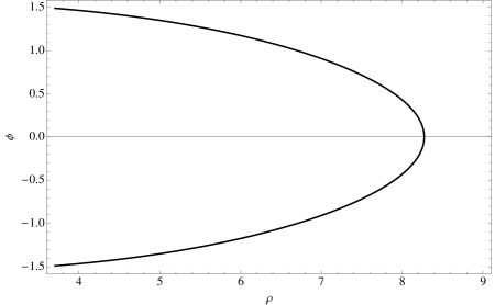
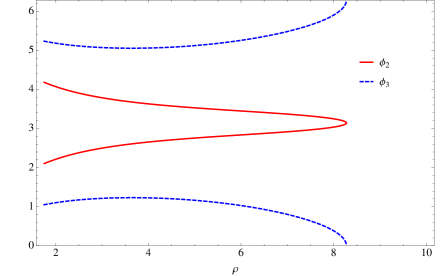
Figure 2: The dependence of $\phi$ and the phases of the heavy Majorana neutrinos on $\rho$ according to eqs. (3.14, 3.15, 3.16). The unit for $\phi,\phi_{2},\phi_{3}$ is rad. We use the best fit values from the global fit [5] for the two squared mass differences as input here.

We comment a little on the phases in the mass matrices. The heavy neutrino mass matrix is diagonalised as

$$U_{\text{GR}}^{\text{T}}M_{\text{RR}}U_{\text{GR}}=D_{N}=\rm\text{Diag}(M_{1}\text{ e}^{\text{i}\phi_{1}},M_{2}\text{ e}^{\text{i}\phi_{2}},M_{3}\text{ e}^{\text{i}\phi_{3}})\;,~{}\quad M_{1,2,3}>0~{}.$$ (3.18)

We eliminate the common phase by setting $\phi_{1}=0$ and attribute the phase factors to a phase matrix $P=\text{Diag}(1,\text{e}^{\text{i}\phi_{2}/2},\text{e}^{\text{i}\phi_{3}/2})$. Thus we have

$$P^{-1}U_{\text{GR}}^{\text{T}}M_{\text{RR}}U_{\text{GR}}P^{-1}=\rm\text{Diag}(M_{1},M_{2},M_{3})\;,$$ (3.19)

which means $U_{\text{GR}}P^{-1}$ diagonalises the heavy neutrino mass matrix to real and non-negative eigenvalues. Applying the seesaw mechanism, we have

$$m_{\text{LL}}=-m_{\text{D}}^{\text{T}}M_{\text{RR}}^{-1}m_{\text{D}}=U_{\nu}^{\star}\text{Diag}(m_{1},m_{2},m_{3})U_{\nu}^{\dagger}~{}.$$ (3.20)

Notice that from $U_{\text{GR}}^{\text{T}}m_{\text{D}}U_{\text{ GR}}=y_{1}^{n}v_{u}\rm\text{Diag}(1,1,-1)+\mathcal{O}(c)$ we get

$$U_{\nu}=\text{i }U_{\text{GR}}P~{}+\mathcal{O}(c).$$ (3.21)

If we choose $y_{1}^{n}$ to be real and positive, the only complexity comes from the heavy neutrino mass matrix and the phase $\gamma$. By ascribing the phases to the $P$ matrix, the $m_{i}$, $i=1,2,3$ in eq. (3.20) are real and non-negative up to corrections of $\mathcal{O}(c)$. From now on, we use the symbol $M_{i}$ and $m_{i}$ to label the real and non-negative masses.

3.2 Leptogenesis

In this section we discuss analytical estimates for the generated baryon asymmetry including all relevant parameters and formulas. To discuss leptogenesis in this model, we first set our scale of interest, the see-saw scale, to be $M_{S}\simeq 10^{13}$ GeV. Taking into consideration $\tan\beta=30$, we have $10^{9}(1+\tan^{2}\beta)$ GeV$<M_{S}<10^{12}(1+\tan^{2}\beta)$ GeV, which as was shown in [15], corresponds to the “two-flavoured leptogenesis” regime [8, 9, 10], i.e., the regime where the processes mediated by the $\tau$ Yukawa couplings enter into equilibrium. Later on in our numerical scan we will find that in order to generate realistic neutrino masses the parameter $\rho$ has to satisfy the inequality $\rho\gtrsim 5.8$. This in turn implies that the leptogenesis regime in the model we are considering cannot be resonant. Indeed, as can be shown, for $\rho\gtrsim 3.7$ we have $M_{1}-M_{2}\gg\Gamma_{1}=\tfrac{(\tilde{Y}_{\nu}\tilde{Y}_{\nu}^{\dagger})_{11}M_{1}}{8\pi}$, the smallest heavy Majorana neutrino mass splitting $(M_{1}-M_{2})$ being by at least two orders of magnitude larger than $\Gamma_{1}$. Thus, the condition of resonant leptogenesis [19] $(M_{1}-M_{2})\sim\Gamma_{1}$, is not satisfied in the model under discussion.

The CP-asymmetry generated in the lepton charge $L_{l}$ by neutrino and sneutrino decays, $l=e,\mu,\tau$, is [13]:

$$\epsilon_{i}^{l}= \frac{1}{8\pi}\frac{1}{(\tilde{Y}_{\nu}\tilde{Y}_{\nu}^{\dagger})_{ii}}\sum_{j\neq i}{\rm Im}[(\tilde{Y}_{\nu})_{jl}(\tilde{Y}_{\nu})_{il}^{\star}(\tilde{Y}_{\nu}\tilde{Y}_{\nu}^{\dagger})_{ji}]f(\tfrac{m_{i}}{m_{j}})$$

$$+\frac{1}{8\pi}\frac{1}{(\tilde{Y}_{\nu}\tilde{Y}_{\nu}^{\dagger})_{ii}}\sum_{j\neq i}{\rm Im}[(\tilde{Y}_{\nu})_{jl}(\tilde{Y}_{\nu})_{il}^{\star}(\tilde{Y}_{\nu}\tilde{Y}_{\nu}^{\dagger})_{ij}]\frac{m_{j}^{2}}{m_{j}^{2}-m_{i}^{2}}~{},$$ (3.22)

where

$$f(x)=-x\left(\frac{2}{x^{2}-1}+\text{log}(1+\frac{1}{x^{2}})\right)~{}.$$ (3.23)

The second term in eq. (3.22) corresponds to the self-energy diagram with an inverted fermion line in the loop. It would vanish when we sum over $\alpha$, and we would end up with the same formula as in the one flavour case

$$\epsilon_{i}=\sum_{l}\epsilon_{i}^{l}=\frac{1}{8\pi}\sum_{j\neq i}\frac{{\rm Im}[(\tilde{Y}_{\nu}\tilde{Y}_{\nu}^{\dagger})_{ji}^{2}]}{(\tilde{Y}_{\nu}\tilde{Y}_{\nu}^{\dagger})_{ii}}f(\tfrac{m_{i}}{m_{j}})~{}.$$ (3.24)

In the basis where the charged lepton and the right handed neutrino mass matrices are diagonal, we have

$$\tilde{Y}_{\nu} =(U_{\text{GR}}P^{-1})^{\dagger}(Y_{\nu}+\delta Y_{\nu})U_{e}$$

$$=y_{1}^{n}\left(\begin{array}[]{ccc}-\frac{\left(s^{e}_{12}\text{e}^{\text{i}\delta_{12}^{e}}+\sqrt{3+\sqrt{5}}c^{e}_{12}\right)}{\sqrt{5+\sqrt{5}}}&\frac{\text{e}^{-\text{i}\delta_{12}^{e}}\left(c^{e}_{12}\text{e}^{\text{i}\delta_{12}^{e}}-\sqrt{3+\sqrt{5}}s^{e}_{12}\right)}{\sqrt{5+\sqrt{5}}}&\frac{1}{\sqrt{5+\sqrt{5}}}\\ \frac{\text{e}^{\frac{\text{i}\phi_{2}}{2}}\left(\left(5+\sqrt{5}\right)\text{e}^{\text{i}\delta_{12}^{e}}s^{e}_{12}-2\sqrt{10}c^{e}_{12}\right)}{2\sqrt{5\left(5+\sqrt{5}\right)}}&-\frac{\text{e}^{\frac{\text{i}\phi_{2}}{2}-\text{i}\delta_{12}^{e}}\left(\left(5+\sqrt{5}\right)c^{e}_{12}\text{e}^{\text{i}\delta_{12}^{e}}+2\sqrt{10}s^{e}_{12}\right)}{2\ 5^{3/4}\sqrt{1+\sqrt{5}}}&-\frac{1}{2}\sqrt{1+\frac{1}{\sqrt{5}}}\text{e}^{\frac{\text{i}\phi_{2}}{2}}\\ -\frac{\text{e}^{\frac{1}{2}\text{i}(2\delta_{12}^{e}+\phi_{3})}s^{e}_{12}}{\sqrt{2}}&\frac{c^{e}_{12}\text{e}^{\frac{\text{i}\phi_{3}}{2}}}{\sqrt{2}}&-\frac{\text{e}^{\frac{\text{i}\phi_{3}}{2}}}{\sqrt{2}}\\ \end{array}\right)$$ (3.28)

$$+y_{1}^{n}c\,\text{e}^{\text{i}\gamma}\left(\begin{array}[]{ccc}-\frac{\left(c^{e}_{12}-\sqrt{3+\sqrt{5}}\text{e}^{\text{i}\delta_{12}^{e}}s^{e}_{12}\right)}{\sqrt{5+\sqrt{5}}}&-\frac{\text{e}^{-\text{i}\delta_{12}^{e}}\left(\sqrt{3+\sqrt{5}}c^{e}_{12}\text{e}^{\text{i}\delta_{12}^{e}}+s^{e}_{12}\right)}{\sqrt{5+\sqrt{5}}}&0\\ \frac{\text{e}^{\frac{\text{i}\phi_{2}}{2}}\left(2\sqrt{2}s^{e}_{12}\text{e}^{\text{i}\delta_{12}^{e}}+\sqrt{5}c^{e}_{12}+c^{e}_{12}\right)}{2\sqrt{5+\sqrt{5}}}&\frac{\text{e}^{\frac{\text{i}\phi_{2}}{2}-\text{i}\delta_{12}^{e}}\left(-2\sqrt{2}c^{e}_{12}\text{e}^{\text{i}\delta_{12}^{e}}+\sqrt{5}s^{e}_{12}+s^{e}_{12}\right)}{2\sqrt{5+\sqrt{5}}}&0\\ \frac{c^{e}_{12}\text{e}^{\frac{\text{i}\phi_{3}}{2}}}{\sqrt{2}}&\frac{\text{e}^{\frac{\text{i}\phi_{3}}{2}-\text{i}\delta_{12}^{e}}s^{e}_{12}}{\sqrt{2}}&0\\ \end{array}\right)~{},$$ (3.32)

where we use $U_{e}\simeq U_{12}$, and the abbreviations $\sin\theta_{12}^{e}=s^{e}_{12}$ and $\cos\theta_{12}^{e}=c^{e}_{12}$.

Here and in the following we have used the freedom to redefine $Y_{\nu}$ by a global phase to make $y_{1}^{n}>0$ so that we find

$$\tilde{Y}_{\nu}\tilde{Y}_{\nu}^{\dagger} =PU_{\text{GR}}^{\text{T}}(Y_{\nu}Y_{\nu}^{\dagger}+Y_{\nu}\delta Y_{\nu}^{\dagger}+\delta Y_{\nu}Y_{\nu}^{\dagger})U_{\text{GR}}P^{-1}$$ (3.33)

$$=\left({y_{1}^{n}}\right)^{2}\mathds{1}+c\left({y_{1}^{n}}\right)^{2}\left(\begin{smallmatrix}0&\text{i}\sqrt{2}\sin\gamma\text{e}^{-\text{i}\phi_{2}/2}&-\sqrt{1+\frac{1}{\sqrt{5}}}\cos\gamma\text{e}^{-\text{i}\phi_{3}/2}\\ -\text{i}\sqrt{2}\sin\gamma\text{e}^{\text{i}\phi_{2}/2}&0&-\frac{2}{\sqrt{5+\sqrt{5}}}\cos\gamma\text{e}^{-\text{i}(\phi_{3}-\phi_{2})/2}\\ -\sqrt{1+\frac{1}{\sqrt{5}}}\cos\gamma\text{e}^{\text{i}\phi_{3}/2}&-\frac{2}{\sqrt{5+\sqrt{5}}}\cos\gamma\text{e}^{\text{i}(\phi_{3}-\phi_{2})/2}&0\\ \end{smallmatrix}\right)~{},$$

which we have expanded up to $\mathcal{O}(c)$.

We give next the expressions for the CP-violating asymmetries in the $l$ lepton charge $L_{l}$, generated in the decays of the heavy Majorana neutrinos $N_{1}$, $N_{2}$ and $N_{3}$, as calculated from eq. (3.22):

$$\epsilon_{1}^{\tau} =\frac{c\left({y_{1}^{n}}\right)^{2}}{8\pi}\frac{1}{\sqrt{10}}\left(\sin\gamma\cos{\phi_{2}}f(\tfrac{m_{1}}{m_{2}})-\sin\gamma\frac{m_{2}^{2}}{m_{2}^{2}-m_{1}^{2}}+\cos\gamma\sin{\phi_{3}}f(\tfrac{m_{1}}{m_{3}})\right)~{},$$ (3.34)

$$\epsilon_{2}^{\tau} =\frac{c\left({y_{1}^{n}}\right)^{2}}{8\pi}\frac{1}{\sqrt{10}}\left(-\sin\gamma\cos{\phi_{2}}f(\tfrac{m_{2}}{m_{1}})+\sin\gamma\frac{m_{1}^{2}}{m_{1}^{2}-m_{2}^{2}}-\cos\gamma\sin{(\phi_{3}-\phi_{2})}f(\tfrac{m_{2}}{m_{3}})\right)~{},$$ (3.35)

$$\epsilon_{3}^{\tau} =\frac{c\left({y_{1}^{n}}\right)^{2}}{8\pi}\frac{1}{\sqrt{10}}\cos\gamma\left(-\sin{\phi_{3}}f(\tfrac{m_{3}}{m_{1}})+\sin{(\phi_{3}-\phi_{2})}f(\tfrac{m_{3}}{m_{2}})\right)~{}.$$ (3.36)

We see that to leading order, $\epsilon_{i}^{\tau}=0$ and hence leptogenesis was not viable in the original model. As $\tilde{Y}_{\nu}$ in leading order is unitary (except for an overall factor $\left({y_{1}^{n}}\right)^{2}$), we have $\epsilon_{i}^{2}\equiv\epsilon_{i}^{e}+\epsilon_{i}^{\mu}=-\epsilon_{i}^{\tau}$ to leading order.

Notice that we compute the CP asymmetry generated by all three heavy (s)neutrino decays since the heavy neutrino spectrum is not very hierarchical in our case.

At the leptogenesis scale and values of $y^{n}_{1}$ of interest, the $\Delta L=2$ processes are negligible. They would be important for a different setup with maximal perturbative values of the Yukawa coupling of interest (say, for $y_{1}^{n}\cong 1$) if the leptogenesis scale would be $10^{14}$ GeV (or for masses of the heavy Majorana neutrinos of the order of $10^{14}$ GeV). Thus, we can use the following analytic approximation for the efficiency factors [10], which accounts for the $\Delta L=1$ interactions and the decoherence effects:

$$\eta(\tilde{m}_{il})\simeq\left(\left(\frac{\tilde{m}_{il}}{8.25\times 10^{-3}\text{ eV}}\right)^{-1}+\left(\frac{0.2\times 10^{-3}\text{ eV}}{\tilde{m}_{il}}\right)^{-1.16}\right)^{-1}~{},$$ (3.37)

where

$$\tilde{m}_{il}=\frac{v_{u}^{2}|(\tilde{Y}_{\nu})_{il}|^{2}}{M_{i}}~{},$$ (3.38)

where we introduce another index $i$, $i=1,2,3$, to label the correspondence to the $i$-th heavy (s)neutrino and $l=e,\mu,\tau$. If we only keep leading order term in $\tilde{m}_{il}$, we will have $\tilde{m}_{i2}\equiv\tilde{m}_{ie}+\tilde{m}_{i\mu}=\frac{v_{u}^{2}{(y_{1}^{n})}^{2}}{M_{i}}-\tilde{m}_{i\tau}$. We list the washout mass parameters as follows

$$\tilde{m}_{1\tau} =\frac{1}{5+\sqrt{5}}\frac{v_{u}^{2}{(y_{1}^{n})}^{2}}{M_{1}}~{},$$ (3.39)

$$\tilde{m}_{2\tau} =\frac{1}{4}\left(1+\frac{1}{\sqrt{5}}\right)\frac{v_{u}^{2}{(y_{1}^{n})}^{2}}{M_{2}}~{},$$ (3.40)

$$\tilde{m}_{3\tau} =\frac{1}{2}\frac{v_{u}^{2}{(y_{1}^{n})}^{2}}{M_{3}}~{}.$$ (3.41)

We do not include the higher order terms $\mathcal{O}(c)$ in the expressions for $\tilde{m}_{il}$ because they generate subleading insignificant corrections.

a

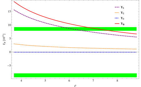
Figure 3: The single asymmetries $Y_{1},Y_{2},Y_{3}$ and the total asymmetry $Y_{B}$. In the upper plot we use $c=0.05\approx\theta_{C}^{2}$, $\gamma=2k\pi~{}(k=0,\pm 1,\pm 2,...)$, $v_{u}=246$ GeV, $y_{1}^{n}=0.1$, $|X|=10^{13}~{}\text{GeV}$ and in the lower plot we use $c=5.8\cdot 10^{-3}\approx\theta_{C}^{5}$, $\gamma=\pi/2+2k\pi$, $v_{u}=246$ GeV, $y_{1}^{n}=0.1$, $|X|=7.2\cdot 10^{12}~{}\text{GeV}$. The horizontal green bands correspond to the 3$\sigma$ region for the observed value for $|Y_{B}|=(8.58\pm 0.22)\times 10^{-11}$, where we multiply for the 3$\sigma$ region the 1$\sigma$ error for the sake of simplicity by a factor of three.

The baryon asymmetry generated by each heavy neutrino decay is [15]

$$Y_{i}\simeq-3\times 10^{-3}\epsilon_{i}^{\tau}\left(\eta\left(\frac{494}{761}\tilde{m}_{i\tau}\right)-\eta\left(\frac{541}{761}\tilde{m}_{i2}\right)\right),$$ (3.42)

and the total baryon asymmetry is

$$Y_{B}=\sum_{i}Y_{i},~{}i=1,2,3.$$ (3.43)

Notice that we use an incoherent sum over the asymmetry generated by each heavy (s)neutrino. This approximation corresponds, in particular, to neglecting the wash-out effects due to the lighter heavy Majorana neutrinos $N_{2,3}$ in the asymmetry generated by the heaviest Majorana neutrino $N_{1}$. Thus, we effectively assume that the indicated wash-out effects cannot reduce drastically the asymmetry produced in the $N_{1}$ decays. Since the masses of $N_{2,3}$ and $N_{1}$ in the model we are considering differ at most by a factor of 5, we can expect that at least for some ranges of values of the masses of $N_{1}$ and $N_{2,3}$ the wash-out effects under discussion will be subdominant, i.e., will lead to a reduction of the asymmetry $Y_{1}$ at most by a factor of 3. Such a reduction will still allow a generation of $Y_{\rm B}$ compatible with the observations. Accounting quantitatively for the wash-out effects of interest requires solving numerically the system of Boltzmann equations describing the evolution of the $N_{1,2,3}$ number densities and of the asymmetries $Y_{1,2,3}$ in the Early Universe. Performing such a calculation is beyond the scope of the present work; it will be done elsewhere.

A priori, we do not know the value of $c\,\text{e}^{\text{i}\gamma}$ introduced in the NLO operator in eq. (2.11). We will see in the next section that the low energy observables combined with $Y_{B}$ will give us information on its value. For now, as interesting cases used for illustration, we plot $Y_{B}$ for some special values of the parameters in Fig. 3. The first set/upper plot will turn out to be not realistic but it is still interesting because here we can see clearly, that the Majorana phases of the heavy right handed neutrinos are the only sources for CP violation and sufficient to generate $Y_{B}$ via leptogenesis. In this case the sign flip of $Y_{1}$ and $Y_{2}$ is due to the loop functions. The sign of $\sin\phi_{i},i=2,3$ can be inferred from the “right sign” observation of $Y_{B}$. The second set/lower plot is inspired by the numerical results later on. Leptogenesis is still successful although there $c$ is chosen much smaller than in the first set, since we receive contribution from the $\sin\gamma$ term, where the enhancement from the loop functions $f(m_{1}/m_{2})$ and $f(m_{2}/m_{1})$ are included. Specifically, we have $f(m_{1}/m_{2})\simeq-30f(m_{1}/m_{3})$ for $\rho=7$. In both cases $Y_{B}$ is dominated by $Y_{1}$. The main difference between $Y_{1}$ and $Y_{2}$ is the efficiency factor: $\eta|_{Y_{1}}/\eta|_{Y_{2}}\simeq 5$ for $\rho=7$. $Y_{3}$ suffers from a strong washout in the first case and is zero in the second case due to $\cos\gamma=0$. The NLO contribution can be regarded as an expansion in powers of $\theta_{C}$ in both cases.

4 Phenomenology: Numerical Results

In this section we discuss the numerical results of a parameter scan. The analytical results give a first impression of the general behaviour of all the observables but since there are several parameters involved which interplay non-trivially we made a random scan of the parameter space with certain assumptions to prove that our model can simultaneously fulfill all the constraints. The structure of this part follows the structure of the previous section.

4.1 Masses and Mixing Angles

For our numerical scan we follow closely the method as described in [2]. Most importantly for the parameters describing the quark and charged lepton sector we used the fit results given there. This implies that we use here $\tan\beta=30$ and $M_{\text{SUSY}}=1$ TeV.

In our previous model we had to scan over four real parameters (two moduli $|X|$ and $|Y|$, two phases $\phi$ and $\delta_{12}^{e}$) in the neutrino sector. In addition to these we have now scanned as well over the modulus $c$ and the phase $\gamma$. And now we have included in our scan as additional constraint [20, 21]

$$Y_{B}=(8.58\pm 0.22)\times 10^{-11}\;,$$ (4.1)

where we multiply for the 3$\sigma$ region the 1$\sigma$ error for the sake of simplicity by a factor of three. For the calculation of $Y_{B}$ we use the formulas from section 3.2.

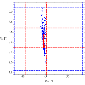
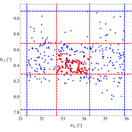
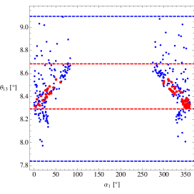
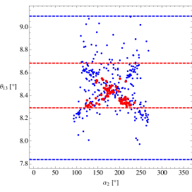
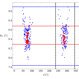
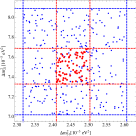
Figure 4: Results of our numerical parameter scan. Blue (red) points are in agreement within 3$\sigma$ (1$\sigma$) of the low energy neutrino masses and mixings and $Y_{B}$ in our model. The allowed experimental 3$\sigma$ (1$\sigma$) regions are limited by blue (red) dashed lines. The black dashed lines represent the 1$\sigma$ range for the not directly measured CP phase $\delta$ from the global fit [5].

Before we come to our results for the normal ordering we want to comment briefly on the inverted ordering. In our numerical scan we were not able to find any points in agreement within 3$\sigma$ with all the mentioned observables. We restricted $c\leq 0.2$ and neglected points where due to a fine-tuned cancellation the NLO corrections were artificially enhanced. Hence, we conclude that this ordering is still excluded like in the original model.

The results of our scan for the masses and mixing angles is shown in Fig. 4 where the careful reader might note first that now we have as well found parameter points that are in agreement within 1$\sigma$ with all observables. That seems to be surprising since we have added here an additional constraint and apart from this expect rather small deviations from the original model. But there are two things coming together: First of all, due to the correction we can now allow for smaller values of $\theta_{23}^{\text{PMNS}}$ down to about $44^{\circ}$ and furthermore we use here the updated results from the nu-fit collaboration [5] which allows for $\theta_{23}^{\text{PMNS}}=45^{\circ}$ even at 1$\sigma$.

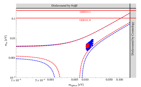
Figure 5: Prediction for the effective neutrino mass $m_{ee}$ accessible in neutrinoless double beta decay experiments as a function of the lightest neutrino mass $m_{1}$. The allowed experimental 3$\sigma$ (1$\sigma$) regions for the masses and mixing angles in the case of normal ordering are limited by blue (red) dashed lines. Blue (red) points are in agreement within 3$\sigma$ (1$\sigma$) of the low energy neutrino masses and mixings and $Y_{B}$ in our model. The grey region on the right side shows the bounds on the lightest mass from cosmology [20] and the grey region in the upper part displays the upper bound on the effective mass from the EXO experiment [22]. The red, straight lines represent the sensitivity of GERDA phase I respectively GERDA phase II [23].

The second thing to note is that now the correlations between $\theta_{13}^{\text{PMNS}}$ and the phases is much weaker which can be explained by the fact that now we have on top another complex parameter in the game. But still the phases are not in arbitrary ranges but we find

$$\delta \in[47^{\circ},104^{\circ}]~{}\text{or}~{}[250^{\circ},316^{\circ}]\;,$$ (4.2)

$$\alpha_{1} \in[0^{\circ},85^{\circ}]~{}\text{or}~{}[275^{\circ},360^{\circ}]\;,$$ (4.3)

$$\alpha_{2} \in[94^{\circ},269^{\circ}]\;,$$ (4.4)

For the Jarlskog invariant which determines the CP violation in neutrino oscillations we find values between $\pm$($0.026-0.035$). The restricted ranges for the phases imply of course also restrictions on the predictions for neutrinoless double beta decay, see Fig. 5. But more restrictive in this case is nevertheless the constraint on the mass scale where the lower bound is mostly determined by the mass sum rule. We obtain for the lightest neutrino mass $m_{1}$ values between 10.5 meV to 17.6 meV. In fact, our prediction for $m_{ee}$ is rather precise to be in the narrow range from 2.3 meV to 9.2 meV. This is way below the sensitivity of any experiment in the near future so that any evidence for neutrinoless double beta decay would rule out this model.

Related to the mass scale are as well two other observables. First of all there is the sum of the neutrino masses

$$\sum m_{\nu}\in(0.074-0.089)~{}\text{eV}\;,$$ (4.5)

which might be determined from cosmology. So far there is only an upper bound [20]

$$\sum m_{\nu}<0.23\text{ eV,}$$ (4.6)

which is well in agreement with our prediction. The second observable is the kinematic mass $m_{\beta}$ as measured in the KATRIN experiment [24] which is given as

$$m_{\beta}^{2}=m_{1}^{2}c_{12}^{2}c_{13}^{2}+m_{2}^{2}s_{12}^{2}c_{13}^{2}+m_{3}^{2}s_{13}^{2}\;.$$ (4.7)

Here we predict $m_{\beta}\approx(0.014-0.019)$ eV which is again way below the projected reach of $m_{\beta}>0.2$ eV.

4.2 Leptogenesis

In this section we show the results of our parameter scan relevant for leptogenesis where we have implemented the formulas given in section 3.2 to calculate the generated baryon asymmetry.

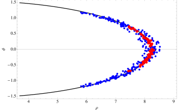
Figure 6: The relation between $\phi$ and $\rho$ according to eq. (3.14) (black line), cf. Fig. 2, and blue (red) points from our numerical scan in agreement within 3$\sigma$ (1$\sigma$) of the low energy neutrino masses and mixings and $Y_{B}$.

Before we actually discuss the results for the asymmetry itself we first want to note that the results from our analytical estimates are quite good. For instance, in Fig. 6 we show the relation between $\phi$ and $\rho$ from eq. (3.14) and from our numerical scan. The agreement is striking although in the analytical estimates we have neglected for instance RGE effects which are nevertheless not very large in the allowed mass range. The biggest difference is in the allowed range for $\rho$. To avoid the resonance condition we only demanded $\rho\gtrsim 3.7$ while we find here $\rho\gtrsim 5.8$. But here not only the ratio of the mass squared differences enter, but the two values of the mass squared differences independently.

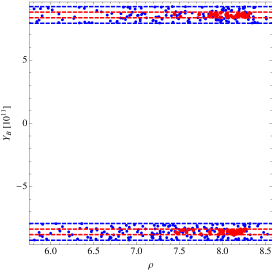
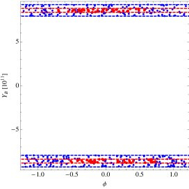
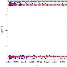
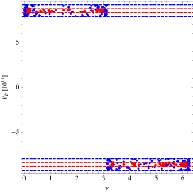
Figure 7: Results of our numerical scan for the total baryon asymmetry $Y_{B}$ in dependence of the four most relevant parameters. Blue (red) points are in agreement within 3$\sigma$ (1$\sigma$) of the low energy neutrino masses and mixings and $Y_{B}$ in our model.

Now that we are convinced that our analytical estimates have been good we discuss the dependence of $Y_{B}$ on the four most relevant parameters as discussed in section 3.2. The biggest advantage of our numerical scan over the analytical estimates is that it allows us to use all available data on neutrino masses and mixing to constrain the allowed parameter space.

We have already seen in Fig. 6 that the values of $\rho$ get constrained which is again visible in Fig. 7. While a priori we only knew that $\rho\gtrsim 3.7$ and less than about 9 we now see that only the range from $5.8$ to $8.5$ is allowed ($7.4-8.3$ at 1$\sigma$). And since $\rho$ and $\phi$ are not independent but related via eq. (3.14), the phase $\phi$ gets constrained as well to the range $[-1.2;1.2]$ ($[-0.5;0.7]$ at 1$\sigma$).

The new parameters $c$ and $\gamma$ are nevertheless more interesting than $\rho$ and $\phi$ which are mostly constrained by the neutrino masses and for which we would have found similar results already in the previous model. In Fig. 7 we have shown the dependence of $Y_{B}$ on this new parameters.

The first thing to note, is that $c$ is indeed a small parameter in the range from $0.7\cdot 10^{-3}$ to $4.9\cdot 10^{-3}$. From the model building point of view such a small value is justified. Remember that the leading order Yukawa coupling is a dimension three operator in the superpotential while the correction proportional to $c$ is coming from a dimension seven operator. Also note that alone from a constraint on $Y_{B}$ $c$ could have been much larger or smaller depending of course on the value of $\gamma$ and the other parameters. This is different here because the mixing angles get corrections of order $c$ and this implies the constraint shown here.

Finally, note that the allowed range for $\gamma$ is only weakly constrained. Nevertheless, it is interesting that the sign of $Y_{B}$ is completely determined by $\gamma$. This is somewhat surprising because in our estimates from section 3.2 the sign of $\epsilon^{\tau}$ depends on other parameters which could induce a sign flip, which can be seen for instance in the upper plot of Fig. 3. But after applying all experimental constraints the correlation is striking.

Combined with the analytic analysis, we see that this correlation is a result of the fact that $Y_{B}$ is dominated by $Y_{1}$, which is again dominated by the first term in $\epsilon_{1}^{\tau}$, where $\cos\phi_{2}$ is negative and $f(m_{1}/m_{2})$ is positive. Neglecting the subdominant terms, we have $Y_{B}\propto\sin\gamma$. The analytical estimates for the efficiency factors we are using provide results with an estimated precision of (20-30)$\%$ compared to the full numerical results solving the Boltzmann equations. This is more than sufficient for the purposes of our study. The other predictions for the light neutrino masses and mixing parameters would only mildly change because they are mostly governed by the leading order values (a 30% correction to $c$ would have only little impact on them). It is also worth mentioning that the complex Yukawa and the Majorana phases are both necessary CP-violating sources to generate a successful baryon asymmetry via leptogenesis while in accordance with all the low energy constraints. It is also noticeable that $Y_{B}$ would be strongly suppressed if $\cos\phi_{2}\cong 0$. As it follows from Fig. 2, values of $\cos\phi_{2}\cong 0$ are excluded in the model we are considering since $\cos\phi_{2}$ can have values only in a narrow interval around $-1$, namely, $(-1,-0.95)$ for $\rho\gtrsim 5.8$, which also means that the Majorana phases contribute maximally to the asymmetry. In order to investigate the role of the Dirac phase we need a different parametrisation of the neutrino Yukawa coupling to see the relation explicitly, which is beyond the scope of the current work.

5 Summary and Conclusions

In this paper we have revised the SU(5) $\times$ A₅ golden ratio GUT flavour model from [2] with the aim to include as well successful leptogenesis. In the original setup this was not possible. As it turns out we only have to add two additional pairs of messenger fields but no additional symmetries or flavon fields to do this. We find that this induces a small correction to the neutrino Yukawa matrix, which can generate a sizeable baryon asymmetry, but as well implies some modifications for the predictions of the masses and mixing angles of the original model. In an extensive numerical scan we could show that we can simultaneously accommodate successfully the observed neutrino masses, mixing angles and possibly baryon asymmetry. And even more our setup is so constrained that we predict several correlations or ranges for observables yet to be measured.

One of the most striking features of our original model - the sum rule for the neutrino masses - remains valid up to a insignificant correction. From this we can again derive a lower bound for the lightest neutrino masses $m_{1}\gtrsim 0.011$ eV and rule out the neutrino mass spectrum with inverted ordering. This is already a very strong prediction.

Due to the additional complex parameter and the additional constraint on $Y_{B}$ the allowed ranges for $\alpha_{2}$ has shrunk from $70^{\circ}-290^{\circ}$ in the original model to $94^{\circ}-269^{\circ}$. Whereas the allowed regions for $\alpha_{1}$ and $\delta$ remain similar compared to the original model. Namely, we find now $\alpha_{1}$ to be in $0^{\circ}-85^{\circ}$ or $275^{\circ}-360^{\circ}$ and $\delta$ to be in $47^{\circ}-105^{\circ}$ or $250^{\circ}-316^{\circ}$. The strong correlation between $\theta_{13}$ and the Majorana phases is now weakened due to the additional complex parameter we introduced in the model. It is also important to note, that we find here points which are in agreement within 1$\sigma$ with all neutrino observables. This is due to the fact that we now allow for smaller values of $\theta_{23}$ but we also use here the updated fit results from [5] where maximal atmospheric mixing is again allowed at the 1$\sigma$ level. Nevertheless, a precise measurement of $\theta_{23}$ which deviates significantly from maximal mixing can rule out the presented model. Since we limit the allowed ranges for the CP violating phases and the light neutrino masses we predict as well the effective Majorana mass observable in neutrinoless double beta decay to be in the narrow range ($2.3-9.2$) meV. This is beyond the reach of ongoing experiments and upcoming experiments which will begin taking data in the near future, but it will be certainly tested in the future.

For the baryon asymmetry $Y_{B}$ we find in the approximation used to calculate it good agreement with the most recent data and this is done by only introducing one additional operator which involves one new complex parameter with a modulus $c$ having a value in the range $0.7\cdot 10^{-3}$ to $4.9\cdot 10^{-3}$. The phase of this additional parameter at the 3$\sigma$ level is not much constrained but it governs the sign of $Y_{B}$.

What we did not discuss in the present article is that some of the features of the original model, like the Yukawa coupling ratios $y_{\tau}/y_{b}\approx-3/2$, remain valid in the modified model implying non-trivial constraints on the spectrum of the supersymmetric partners of the Standard Model particles.

In summary we have succeeded to modify the model from [2] to include viable leptogenesis by only introducing a minimal correction. The model presented here is, to our knowledge, the first GUT $\text{A}_{5}$ golden ratio flavour model in which it is possible to have successful leptogenesis. All observables lie within the measured ranges and for the not yet measured quantities in the neutrino sector (the type of the neutrino mass spectrum, the absolute scale and the sum of the neutrino masses, the effective Majorana mass in neutrinoless double beta decay, the CP violation phases in the PMNS matrix), we make predictions. An appealing feature of the model is its rather small number of parameters, which makes the model very predictive and testable.

References

- [1] M. Fukugita and T. Yanagida, Phys. Lett. B 174 (1986) 45.
- [2] J. Gehrlein, J. P. Oppermann, D. Schäfer and M. Spinrath, Nucl. Phys. B 890 (2015) 539 [arXiv:1410.2057 [hep-ph]].
- [3] A. Datta, F. -S. Ling and P. Ramond, Nucl. Phys. B 671 (2003) 383 [hep-ph/0306002]. L. L. Everett and A. J. Stuart, Phys. Rev. D 79 (2009) 085005 [arXiv:0812.1057 [hep-ph]]; F. Feruglio and A. Paris, JHEP 1103 (2011) 101 [arXiv:1101.0393 [hep-ph]]. Y. Kajiyama, M. Raidal and A. Strumia, Phys. Rev. D 76 (2007) 117301 [arXiv:0705.4559 [hep-ph]]. I. K. Cooper, S. F. King and A. J. Stuart, Nucl. Phys. B 875 (2013) 650 [arXiv:1212.1066 [hep-ph]]. C. H. Albright, A. Dueck and W. Rodejohann, Eur. Phys. J. C 70 (2010) 1099 [arXiv:1004.2798 [hep-ph]].
- [4] J. Beringer et al. [Particle Data Group Collaboration], Phys. Rev. D 86 (2012) 010001.
- [5] M. C. Gonzalez-Garcia, M. Maltoni and T. Schwetz, JHEP 1411 (2014) 052 [arXiv:1409.5439 [hep-ph]].
- [6] S. Antusch and M. Spinrath, Phys. Rev. D 79 (2009) 095004; [arXiv:0902.4644 [hep-ph]]; S. Antusch, S. F. King and M. Spinrath, Phys. Rev. D 89 (2014) 055027 [arXiv:1311.0877 [hep-ph]].
- [7] S. Antusch and V. Maurer, Phys. Rev. D 84 (2011) 117301 [arXiv:1107.3728 [hep-ph]]; D. Marzocca, S. T. Petcov, A. Romanino and M. Spinrath, JHEP 1111 (2011) 009 [arXiv:1108.0614 [hep-ph]]; S. Antusch, C. Gross, V. Maurer and C. Sluka, Nucl. Phys. B 866 (2013) 255; [arXiv:1205.1051 [hep-ph]]].
- [8] E. Nardi, Y. Nir, E. Roulet and J. Racker, JHEP 0601 (2006) 164 [hep-ph/0601084].
- [9] A. Abada, S. Davidson, F. X. Josse-Michaux, M. Losada and A. Riotto, JCAP 0604 (2006) 004 [hep-ph/0601083].
- [10] A. Abada, S. Davidson, A. Ibarra, F.-X. Josse-Michaux, M. Losada and A. Riotto, JHEP 0609 (2006) 010 [hep-ph/0605281].
- [11] S. Pascoli, S. T. Petcov and A. Riotto, Phys. Rev. D 75 (2007) 083511 [hep-ph/0609125].
- [12] G. C. Branco, R. Gonzalez Felipe and F. R. Joaquim, Phys. Lett. B 645 (2007) 432 [hep-ph/0609297].
- [13] S. Davidson, E. Nardi and Y. Nir, Phys. Rept. 466 (2008) 105 [arXiv:0802.2962 [hep-ph]].
- [14] G. C. Branco, R. G. Felipe and F. R. Joaquim, Rev. Mod. Phys. 84 (2012) 515 [arXiv:1111.5332 [hep-ph]].
- [15] S. Pascoli, S. T. Petcov and A. Riotto, Nucl. Phys. B 774 (2007) 1 [hep-ph/0611338].
- [16] C. Hagedorn, E. Molinaro and S. T. Petcov, JHEP 0909 (2009) 115 [arXiv:0908.0240 [hep-ph]].
- [17] S. T. Petcov, Nucl. Phys. B 892 (2015) 400 [arXiv:1405.6006 [hep-ph]].
- [18] S. Antusch and S. F. King, Phys. Lett. B 631 (2005) 42 [hep-ph/0508044].
- [19] A. Pilaftsis, Phys. Rev. D 56 (1997) 5431 [hep-ph/9707235].
- [20] P. A. R. Ade et al. [Planck Collaboration], arXiv:1303.5076 [astro-ph.CO].
- [21] C. L. Bennett et al. [WMAP Collaboration], Astrophys. J. Suppl. 208 (2013) 20 [arXiv:1212.5225 [astro-ph.CO]].
- [22] J. B. Albert et al. [EXO-200 Collaboration], Nature 510 (2014) 229-234 [arXiv:1402.6956 [nucl-ex]].
- [23] A. A. Smolnikov [GERDA Collaboration], arXiv:0812.4194 [nucl-ex].
- [24] J. Angrik et al. [KATRIN Collaboration], FZKA-7090.