Order statistics inference for describing topological coupling and mechanical symmetry breaking in multidomain proteins

Abstract

Cooperativity is a hallmark of proteins, many of which show a modular architecture comprising discrete structural domains. Detecting and describing dynamic couplings between structural regions is difficult in view of the many-body nature of protein-protein interactions. By utilizing the GPU-based computational acceleration, we carried out simulations of the protein forced unfolding for the dimer $WW$$-$$WW$ of the all-$\beta$-sheet $WW$ domains used as a model multidomain protein. We found that while the physically non-interacting identical protein domains ($WW$) show nearly symmetric mechanical properties at low tension, reflected, e.g., in the similarity of their distributions of unfolding times, these properties become distinctly different when tension is increased. Moreover, the uncorrelated unfolding transitions at a low pulling force become increasingly more correlated (dependent) at higher forces. Hence, the applied force not only breaks “the mechanical symmetry” but also couples the physically non-interacting protein domains forming a multi-domain protein. We call this effect “the topological coupling”. We developed a new theory, inspired by Order statistics, to characterize protein-protein interactions in multi-domain proteins. The method utilizes the squared-Gaussian model, but it can also be used in conjunction with other parametric models for the distribution of unfolding times. The formalism can be taken to the single-molecule experimental lab to probe mechanical cooperativity and domain communication in multi-domain proteins.

I INTRODUCTION

Mechanical forces play an important role in life processes, and many biological molecules are subjected to forces. There are numerous examples from biology, where mechanical forces play an essential role in a physiological context. Tensile forces acting on cells or bacteria originate from the dragging forces imposed by the fluid flow Puchner and Gaub (2009). A function of a biological motor might result in the generation of large pulling force. For example, active force from myosin generates substantial mechanical stress on structures of the sarcomere Gautel (2011); Kasza and Zallen (2011). Mechanical forces can also be generated within the biological system. For example, leukocytes that patrol the blood flow in search of pathogens, need to generate internal force to squeeze into in and pass through connective tissues Rodger P (2002). In addition to biochemical stimuli, cellular processes involving the cytoskeleton can be modulated in response to external force Kasza and Zallen (2011).

Structural arrangements of proteins have evolved in response to the selection pressure from biological forces. The three-dimensional structures often exhibit a modular architecture composed of discrete structural regions. These include semi-static structures such as actin filaments and microtubules, and flexible structures such as muscle protein titin and fibrin clot Nakamura et al. (2011); Tskhovrebova and Trinick (2010); Weisel (2008). Titin, a giant $1\mu m$ protein formed by linked immunoglobulin and fibronectin domains defines the structure and elasticity of muscle sarcomere Tskhovrebova and Trinick (2010); Gautel (2011). Proteins that form or interact with the extracellular matrix (ECM) have modular or multidomain architecture Leckband and Sivasankar (2012); Ramage (2012). These include fibronectin fibrils, which form meshworks around the cell, and integrins, which link the cell external and intracellular environment Wang et al. (2009). Fibrin polymerization in blood results in formation of branched network called a fibrin clot, which must sustain large shear stress due to blood flow Weisel (2008); Brown et al. (2009). Protein shells of plant and animal viruses (capsids) are often made of multiple copies of a single structural unit (capsomer). For example, the capsid of Cowpea Chlorotic Mottle Virus is an icosahedral shell comprised of $180$ copies of a single ($190$ amino acid) protein Speir et al. (1995).

Physical properties of proteins have adapted to biological forces. In ECM assembly, fibronectin subunits change conformations from compact to extended. The extent of assembly is controlled by cell contractility through actin filaments Singh et al. (2010). Hence, tissue tension regulate matrix assembly. Virus capsids should be stable enough to protect encapsulated material (DNA or RNA), yet, unstable to release the material when invading their host cells Roos et al. (2010). Hence, mechanical properties of virus capsids are important factors in viruses’ survival in the extracellular environment and cell infectivity. Cell adhesion and migration rely on reversible changes in mechanical properties of cells. Spatial distribution of internal tension in cell remodeling, derived from dynamic regulation of contractile actin-myosin networks, correlates cell shape and movement Lieleg et al. (2010); Kasza and Zallen (2011). In addition, many proteins have evolved to act as “force sensors” to convert tension-induced conformational changes into biological signal Wang et al. (2009). For example, tissue deformation during mechanical stimulation alters the conformation of ECM molecules. Filamins involved in mechanotransduction alter their structure in response to external tension Sutherland-Smith (2011). Proper communication between structural regions in multidomain proteins is important for regulation. For example, dynamic coupling between the regulatory domain and the ligand-binding domain in P-selectins is implicated in formation of force-activated bonds Hertig and Vogel (2012) (“catch bonds” Barsegov and Thirumalai (2006)) with their ligands (PSGL-1).

Single-molecule experimental techniques such as Atomic Force Microscopy (AFM) Puchner and Gaub (2009); $\breve{Z}$oldak and Rief (2013); Lannon et al. (2012) and optical trap Fazal and Block (2011); $\breve{Z}$oldak and Rief (2013), have made it possible to study life processes at the level of individual molecules. These experiments, which utilize mechanical force to unfold proteins or to dissociate protein-protein complexes, have made it possible to probe the unfolding or unbinding transitions one at a time Litvinov et al. (2012). In the context of protein forced unfolding, grabbing the molecule at specific positions allows one to select specific region(s) of the molecule and to define the unfolding reaction coordinate. Mechanical manipulation continues to provide a unique approach to quantify the unfolding transitions in terms of the measurable quantities - the unfolding forces (constant velocity or force-ramp experiment) and the unfolding times (constant force or force-clamp experiment). Consider a force-clamp experiment on a multimeric protein $D_{n}$ formed by head-to-tail connected identical domains ($D$’s). The protein is subjected to the external pulling force, and each unfolding transition causes an increase in the chain length, $\Delta Y$. As a result, the total length of the polypeptide chain $Y$ shows the characteristic pattern of stepwise increases ($\Delta Y$’s), which mark sequential unfolding transitions in protein domains.

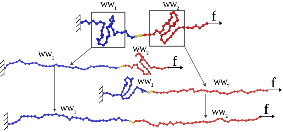
Figure 1: (Olga Kononova, Lee Jones, Valeri Barsegov)

The goal of statistical analysis and modeling of force spectroscopy data is to obtain accurate information about the physical characteristics of protein domains. Yet, due to inherent limitations in the current experimental resolution, there is no direct way of attributing the times of transitions to the protein domains or structural regions where these transitions have occurred. We only have partial or incomplete observation of the system. Said differently, it is not possible to determine which specific domain has unfolded at any time since any domain can unfold at any given time. Consider the simplest case of the dimer $WW$$-$$WW$ of the $WW$ domain, presented in Fig. 1. There are two possible scenarios of unfolding. In the first pathway, the first domain ($WW_{1}$) unfolds first and the second domain ($WW_{2}$) unfolds second. In the second pathway, the order of unfolding is reversed. In an experimental measurement, what is being recorded is the first unfolding time ($t_{1:2}$) and the second unfolding time ($t_{2:2}$) in a sequence of two observations, and it is impossible to tell which domain has unfolded first or second. Hence, the first unfolding times ($t_{1:2}$) and the second unfolding times ($t_{2:2}$) involve contributions from the first domain $WW_{1}$, which unfolds at time $t_{1}$, and the second domain $WW_{2}$, which unfolds at time $t_{2}$. Can we obtain domain-specific information from the experimental data?

The first step is to understand the nature of the random variables measured. In a constant force experiment on an $n$-domain protein ($D_{1}$$-$$D_{2}$$-$$\ldots$$D_{n}$), individual domains unfold one after another but any domain can unfold at any given time. The observed unfolding times are ordered, i.e. they comprise a set of ordered time variates, also known as Order statistics Gumbel (2004); David and Nagaraja (2003). Hence, what is being measured are the “time-ordered data” $t_{1:n},t_{2:n},\ldots,t_{n:n}$, where $t_{r:n}$ is the $r$-th unfolding time ($r$$=$$1,2,\ldots,n$) (in a sequence of $n$ observations). These are different from the (hidden) “parent data” $t_{1},t_{2},\ldots,t_{n}$ with $t_{i}$ being the unfolding time of the $i$-th domain ($D_{i}$, $i$$=$$1,2,\ldots,n$), which contain information about the individual protein domains ($D_{1},D_{2},\ldots,D_{n}$). Hence, the question becomes - can we solve an inverse problem, namely, can we perform the inference of the parent distributions of unfolding times from the distributions of (observed) ordered unfolding times?

The $r$-th order statistic is characterized by the cumulative distribution functions (cdf’s) $P_{r:n}(t)$, and the probability density functions (pdf’s) $p_{r:n}(t)$ of the $r$-th unfolding time, $r$$=$$1,2,\dots,n$, in a sequence of $n$ observations (for $n$ domains). The $r$-th order statistic cdf $P_{r:n}(t)$ is the probability that the $r$-th unfolding time $t_{r}$ does not exceed $t$, i.e., $P_{r:n}(t)$$=$$Prob(t_{r}\leq t)$, and the $r$-th order statistic pdf is $p_{r:n}(t)$$=$$dP_{r:n}(t)/dt$ Gumbel (2004). In our example for the dimer $WW$$-$$WW$, the first unfolding time ($t_{1:2}$) and the second unfolding time ($t_{2:2}$) both carry information about the unfolding times for the first domain $WW_{1}$ ($t_{1}$) and for the second domain $WW_{2}$ ($t_{2}$). In general, because the cdf $P_{r:n}(t)$ and the pdf $p_{r:n}(t)$ of the $r$-th order statistic depend on the parent cdf $P_{i}(t)$ and pdf $p_{i}(t)$ ($i$$=$$1,2,\ldots,n$), it is possible, at least in principle, to resolve $P_{i}(t)$ and $p_{i}(t)$ from the cdf and pdf of the order statistics, $P_{r:n}(t)$ and $p_{r:n}(t)$.

In our recent papers Bura et al. (2007a, b), we used Order statistics to solve the inverse problem for the independent identically distributed (iid) random variables and for the independent non-identically distributed (inid) random variables. The formalism presented in these papers can be used to describe the physically non-interacting identical protein domains ($D$’s) forming a multimeric protein $D$$-$$D$$-$$\ldots$$-$$D$ (iid case), and the non-interacting non-identical domains ($D_{i}$’s, $i$$=$$1,2,\ldots,n$) forming a multi-domain protein $D_{1}$$-$$D_{2}$$-$$\ldots$$-$$D_{n}$ (inid case) Bura et al. (2007a). We have designed rigorous statistical tools for assessing the independence of the parent forced unfolding times ($t_{i}$) and the equality of the parent pdfs of unfolding times ($p_{i}(t)$) from the observed ordered unfolding times ($t_{r:n}$) Bura et al. (2007b). These statistical tests can be utilized to classify the parent unfolding times and to detect correlated unfolding transitions in multi-domain proteins using experimental force spectroscopy data. We have also extended Order statistics approach to describe the unfolding forces measured in the constant-velocity (force-ramp) experiments Zhmurov et al. (2010a). Order statistics inference methods have been applied successfully to inverse problems involving, e.g., partialy observed queuing systems Jones (2013); Jones and Larson (1995); Larson (1990).

Here we take a step further and present a new theory inspired by Order statistics, to solve the inverse problem for the dependent identically distributed (did) random variables and for the dependent non-identically distributed (dnid) random variables, using a squared-Gaussian parametric model of the distributions of unfolding times. The developed formalism can be used to describe the mechanical behavior of interacting (coupled) identical protein domains in a multimeric protein $D$$-$$D$$-$$\ldots$$-$$D$ (did case), and interacting non-identical domains in a multidomain protein $D_{1}$$-$$D_{2}$$-$$\ldots$$-$$D_{n}$ (dnid case). In the next Section, we describe our method. We focus on the order statistics pdf’s, since these statistical measures can be easily estimated by constructing the histograms of unfolding times. We establish a relashionship between the order statistics pdf’s and the parent pdf’s. In Section III, we describe the Self Organized Polymer (SOP) model of the all-$\beta$-sheet $WW$ domain and Langevin simulations of the forced unfolding of the dimer $WW$$-$$WW$ used as a model system (Fig. 1). The in silico experiments mimic single-molecule measurements in vitro Zhmurov et al. (2011a); Zhmurov et al. (2012); Theisen et al. (2012); Duan et al. (2011). In section IV, we perform a direct statistical analysis of the simulation output for dimer $WW$$-$$WW$ and describe the effects of “mechanical symmetry breaking” and “topological coupling”. In Section V, we compare several statistical measures of the ”parent data” for each $WW$ domain - the distribution of unfolding times, the average unfolding time, the standard deviation, and the skewness of distribution, and Pearson correlation coefficient, with the same measures obtained by applying Order statistics inference to the “time-ordered data”. We discuss our results in Section VI.

II ORDER STATISTICS INFERENCE

Consider a vector of order statistics ${\bf T^{\prime}}$$=$$[t_{1:n},t_{2:n},\dots,t_{n:n}]^{\dagger}$, in which the entries obtained in a single measurement correspond to the $1$-st unfolding time ($t_{1:n}$), $2$-nd unfolding time ($t_{2:n}$), $\dots$, and $n$-th unfolding time ($t_{n:n}$), the symbol “dagger” ($\dagger$) represents vector transpose ($t_{r:n}$ denotes the $r$-th unfolding time out of $n$ times for a protein $D_{1}$$-$$D_{2}$$-$$\ldots$$-$$D_{n}$ of $n$ domains $D_{1},D_{2},\ldots,D_{n}$). This same observation ${\bf T^{\prime}}$ can be also obtained by rearranging the components of another vector ${\bf T}$$=$$[t_{1},t_{2},\dots,t_{n}]^{\dagger}$ in the order of increasing time variates, which represents the unfolding times of the $1$-st domain $D_{1}$ ($t_{1}$), $2$-nd domain $D_{2}$ ($t_{2}$), $\dots$, and $n$-th domain $D_{n}$ ($t_{n}$) of the same multidomain protein $D_{1}$$-$$D_{2}$$-$$\ldots$$-$$D_{n}$. This is because any domain can unfold at any given time with a non-zero probability and, hence, there are multiple unfolding scenarios. Hence, on the one hand, we observe the “time-ordered data” ($t_{r:n}$), and on the other hand, we have (hidden) ”parent data” ($t_{i}$). We call this transformation map ${\bf G}$ and write ${\bf T^{\prime}}$$=$${\bf G}({\bf T})$$=$$[t_{1:n},t_{2:n},\dots,t_{n:n}]^{\dagger}$, where $t_{r:n}$ is the $r$-th smallest component of vector ${\bf T}$.

Let vector ${\bf T^{\prime}}$ have the joint pdf $p_{\bf T^{\prime}}(t_{1:n},t_{2:n},\dots,t_{n:n})$ and let vector T have the joint pdf $p_{\bf T}(t_{1},t_{2},\dots t_{n})$. We seek to establish a relationship between the pdf of the ordered data, $p_{\bf T^{\prime}}(t_{1:n},t_{2:n},\dots,t_{n:n})$, and the pdf of the parent data, $p_{\bf T}(t_{1},t_{2},\dots t_{n})$. Let us first assume, that vector ${\bf T}$ can be written as ${\bf T}$$=$$[t_{1},t_{2},\dots,t_{n}]^{\dagger}$$=$$[x_{1}^{2},x_{2}^{2},\dots,x_{n}^{2}]^{\dagger}$, where ${\bf X}$$=$$[x_{1},x_{2},\dots,x_{n}]^{\dagger}$ is an arbitrary random vector sampled from the Gaussian distribution

$$p_{\bf X}(x_{1},x_{2},\dots,x_{n})=\frac{1}{(2\pi)^{n/2}\sqrt{|{\bf{\bf\Sigma}}}|}e^{-\frac{1}{2}({\bf X}-{\bf\mu})^{\dagger}{\bf\Sigma}^{-1}({\bf X}-{\bf\mu})}$$ (1)

where ${\bf\mu}$$=$$[\mu_{1},\mu_{2},\dots,\mu_{n}]^{\dagger}$ is the vector of the mean, and ${\bf\Sigma}$$=$$[\sigma_{ij}]_{i,j=1}^{n}$ is the covariance matrix of vector ${\bf X}$. Here, $|{\bf\Sigma}|$ denotes the determinant of matrix ${\bf\Sigma}$. We use squared-Gaussian distribution since it yields one-sided exponential tail behavior and a non-zero skewness (typical of Gamma-process), but unlike Gamma distribution, squared-Gaussian is simple to describe correlations of the data.

We next obtain the joint probability density function of the parent data ${\bf T}$ in terms of the random variable ${\bf X}$, by using the following general transformation formula for the joint pdf of the multivariate random variable:

$$p_{{\bf T}}(t_{1},t_{2},\dots,t_{n})=\sum_{l}{p_{{\bf X}}(x^{l}(t_{1},t_{2},\dots,t_{n}))}||{\bf J}^{l}(t_{1},t_{2},\dots,t_{n})||$$ (2)

which is valid for a smooth many-to-one mapping from real space $R^{n}$ to real space $R^{n}$ with the non-zero Jacobian of the inverse mapping. In Eq. (2), the sum runs over all inverse branches, $x^{l}(t_{1},t_{2},\dots,t_{n})$, with $l$ being the $l$-th branch, and $||{\bf J}^{l}||=\Bigl{|}\det\left[\frac{\partial x_{i}^{l}({\bf t})}{\partial t_{j}}\right]_{i,j=1}^{n}\Bigr{|}$ is the absolute value of the Jacobian of the $l$-th inverse branch. The total number of inverse branches for the transformation $t_{i}$$=$$x_{i}^{2}$ ($i$$=$$1,2,\dots,n$) is $2^{n}$, and they can be written as $x_{i}^{l}$$=$$s_{i}^{l}\sqrt{t_{i}}$, $s_{i}^{l}$$=$$\pm 1$, $l$$=$$1,2,\dots,2^{n}$ ($i$$=$$1,2,\dots,n$). The Jacobian matrix for this transformation is given by a diagonal matrix, with the $i$-th diagonal entry given by $J_{i}^{l}$$=$$\frac{s_{i}^{l}}{2\sqrt{t_{i}}}$. The determinant of this matrix is $|{\bf J}^{l}|$$=$$\prod_{i=1}^{n}{\frac{s_{i}^{l}}{2\sqrt{t_{i}}}}$. Substituting the expressions for $p_{\bf X}$ and $|{\bf J}^{l}|$ in Eq. (2), we arrive at the joint pdf of the parent data expressed in terms of the pdf of vector ${\bf X}$:

$$p_{{\bf T}}(t_{1},t_{2},\dots,t_{n})=\frac{1}{(2\pi)^{n/2}\sqrt{|{\bf\Sigma}|}}\cdot\frac{1}{2^{n}\sqrt{t_{1}\cdot t_{2}\cdots t_{n}}}\sum_{\bf s}{e^{-\frac{1}{2}({\bf s}{\bf\sqrt{T}}-{\bf\mu})^{\dagger}{\bf\Sigma}^{-1}({\bf s}{\bf\sqrt{T}}-{\bf\mu})}}$$ (3)

where the sum varies over all vectors of signs ${\bf s}$$=$$[s_{1},s_{2},\dots,s_{n}]^{\dagger}$ with the entries $s_{i}$$=$$\pm$$1$, and ${\bf s}{\bf\sqrt{T}}$$=$$[s_{1}\sqrt{t_{1}},s_{2}\sqrt{t_{2}},\dots,s_{n}\sqrt{t_{n}}]^{\dagger}$ is the vector of inverse transformation written in terms of the components ($i$$=$$1,2,\dots,n$).

The final step is to obtain the pdf of the time-ordered data, $p_{\bf T^{\prime}}(t_{1:n},t_{2:n},\dots,t_{n:n})$, in terms of the pdf of the parent data using Eq. (2). Consider the map ${\bf G}$, and use this map in Eq. (2). Since ${\bf G}$ orders the components of vector ${\bf T}$ to produce the order statistics vector ${\bf T^{\prime}}$$=$$[t_{1:n},t_{2:n},\dots,t_{n:n}]^{\dagger}$, the inverse branches of ${\bf G}$ are all possible permutations, $\kappa$, of the components of vector ${\bf T^{\prime}}$. In the case of $n$ domains, there are a total of $n!$ possible rearrangements of $n$ components and, hence, $n!$ of the inverse branches of ${\bf G}$. Since the Jacobian of the permutation transformation is either $+1$ or $-1$, the formula connecting the joint pdf of the order statistics data and the joint pdf of the parent data reads:

$$p_{{\bf T}^{\prime}}(t_{1:n},t_{2:n},\dots,t_{n:n}) = \sum_{\kappa}{p_{{\bf T}}(t_{\kappa(1):n},t_{\kappa(2):n},\dots,t_{\kappa(n):n})}$$ (4)

$$= \frac{1}{(2\pi)^{n/2}\sqrt{|{\bf\Sigma}|}}\cdot\frac{1}{2^{n}\sqrt{t_{1:n}\cdot t_{2:n}\cdots t_{n:n}}}\sum_{\kappa}{\sum_{\bf s}{e^{-\frac{1}{2}({\bf s}{\bf\sqrt{T_{\kappa}}}-{\bf\mu})^{\dagger}{\bf\Sigma}^{-1}({\bf s}{\bf\sqrt{T_{\kappa}}}-{\bf\mu})}}}$$

where the symbolic summation is performed over all possible permutations of components of vector ${\bf T^{\prime}}$, denoted as $\kappa$, and $\bf s\sqrt{T_{\kappa}}$$=$$[s_{1}\sqrt{t_{\kappa(1):n}},s_{2}\sqrt{t_{\kappa(2):n}},\dots,s_{n}\sqrt{t_{\kappa(n):n}}]^{\dagger}$ is a vector of inverse branches of transformations $t_{i}$$=$$x_{i}^{2}$ and ordering G. The expression in the second line of Eq. (4) has $2n+n(n-1)/2$ unknown parameters, including $n$ components of the vector of the mean (${\bf\mu}$$=$$[\mu_{1},\mu_{2},\dots,\mu_{n}]^{\dagger}$), and $(n^{2}+n)/2$ entries of the symmetric covariance matrix (${\bf\Sigma}$$=$$[\sigma_{ij}]_{i,j=1}^{n}$). One can use any estimation method to determine these parameters. Given the statistics of $x_{i}$ ($\mu_{i}$ and $\sigma_{ij}$), we can obtain the pdf ($p_{i}(t)$), the mean ($\mu_{i}^{T}$), the variance ($\sigma_{i}^{T}$), the skewness of distribution ($\gamma_{i}^{T}$) for $t_{i}$ ($i$$=$$1,2$), and estimate pair-wise correlations ($\rho_{ij}^{T}$) using the analysis in the Appendix, which treats the case of $i,j$$=$$1,2$.

III FORCE-CLAMP MEASUREMENTS in silico

III.1 Computer model of dimer $WW$$-$$WW$

We used the $C_{\alpha}$-based Self Organized Polymer (SOP) model of the polypeptide chain Hyeon et al. (2006) to describe the dimer $WW$$-$$WW$ formed by the all-$\beta$-sheet $WW$ domains (Fig. 1). The $WW$ domain has $34$ amino acid residues (Protein Data Bank (PDB) entry 1PIN Koepf et al. (1999)). The mechanical unraveling of $WW$ is described by the single-step kinetics of unfolding, $F\rightarrow U$, from the folded state $F$ to the unfolded state $U$. The dimer $WW$$-$$WW$ was constructed by connecting the N- and C-termini of the adjacent $WW$ domain using flexible linkers of two and four neutral residues (Fig. 1). Each residue in $WW$$-$$WW$ was represented by its $C_{\alpha}$-atom with the $C_{\alpha}$$-$$C_{\alpha}$ covalent bond distance of $a$$=$$3.8\AA$ (peptide bond length).

The molecular potential energy of a protein conformation, specified in terms of the residue coordinates $\{{\bf r}_{i}\}$, $i$$=$$1,2,\dots,M$, is given by

$$V_{MOL} = V_{FENE}+V^{ATT}_{NB}+V^{REP}_{NB}$$ (5)

$$= -\sum_{i=1}^{M-1}{\frac{k}{2}R_{0}^{2}\log{\left(1-\frac{\left(r_{i,i+1}-r^{0}_{i,i+1}\right)^{2}}{R_{0}^{2}}\right)}}$$

$$+ \sum_{i=1}^{M-3}\sum_{j=i+3}^{M}\varepsilon_{h}\left[\left(\frac{r^{0}_{ij}}{r_{ij}}\right)^{12}-2\left(\frac{r^{0}_{ij}}{r_{ij}}\right)^{6}\right]\Delta_{ij}$$

$$+ \sum_{i=1}^{M-2}\varepsilon_{l}\left(\frac{\sigma}{r_{i,i+1}}\right)^{6}+\sum_{i=1}^{M-3}\sum_{j=i+3}^{M}\varepsilon_{l}\left(\frac{r^{0}_{ij}}{r_{ij}}\right)^{6}(1-\Delta_{ij})$$

where the distance between any two interacting residues $i$ and $i$$+$$1$ is $r_{i,i+1}$, whereas $r^{0}_{i,i+1}$ is its value in the native structure. The first term in Eq. (5) is the FENE potential, which describes the chain connectivity; $R_{0}$$=$$2\AA$ is the tolerance in the change of a covalent bond ($k$$=$$1.4N/m$). The second term is the Lennard-Jones potential ($V_{NB}^{ATT}$), which accounts for the native interactions. We assumed that if the non-covalently linked residues $i$ and $j$ ($|i-j|$$>$$2$) are within the cutoff distance in the native state $r_{C}$$=$$8.0\AA$, then $\Delta_{ij}$$=$$1$ and zero otherwise. We used a uniform value of $\varepsilon_{h}$$=$$1.5kcal/mol$, which specifies the strength of the non-bonded interactions. All the non-native interactions were treated as repulsive ($V_{NB}^{REP}$). An additional constraint was imposed on the bond angle between residues $i$, $i$$+$$1$, and $i$$+$$2$ by including the repulsive potential with parameters $\varepsilon_{l}$$=$$1kcal/mol$ and $\sigma$$=$$3.8\AA$, which quantify the strength and the range of repulsion. To ensure the self-avoidance of the protein chain, we set $\sigma$$=$$3.8\AA$.

III.2 Simulations of forced unfolding of dimer $WW$$-$$WW$

The unfolding dynamics were obtained by integrating the Langevin equations for each particle position ${\bf r}_{i}$ in the over-damped limit, $\eta d{\bf r}_{i}/dt$$=$$-\partial V/\partial{\bf r}_{i}$$+$${\bf g}_{i}(t)$. Here, $V$$=$$V_{MOL}$$-$${\bf f}$${\bf Y}$ is the total potential energy, in which the first term ($V_{MOL}$) is the molecular contribution (see Eq. (5)) and the second term represents the influence of applied force on the molecular extension ${\bf Y}$. Also, ${\bf g}­(t)$ is the Gaussian distributed random force and $\eta$ is the friction coefficient. In each simulation run, the N-terminal $C_{\alpha}$-atom of the first domain ($WW_{1}$) was constrained and a constant force ${\bf f}$$=$$f$${\bf n}$ was applied to the C-terminal $C_{\alpha}$-atom of the second domain ($WW_{2}$) in the direction ${\bf n}$ of the end-to-end vector of the dimer ${\bf Y}$ (see Fig. 1). The Langevin equations were propagated with the time step $\Delta t$$=$$0.08$$\tau_{H}$$=$$20ps$, where $\tau_{H}$$=$$\zeta$$\varepsilon_{h}$$\tau_{L}/k_{B}T$. Here, $\tau_{L}$$=$$(ma^{2}/\varepsilon_{h})^{1/2}$$=$$3ps$, $\zeta$$=$$50$ is the dimensionless friction constant for a residue in water ($\eta$$=$$\zeta m/\tau_{L}$), and $m$$\approx$$3$$\times$$10^{-22}g$ is the residue mass Veitshans et al. (1997). Pulling simulations were carried out at room temperature using the bulk water viscosity, which corresponds to the friction coefficient $\eta$$=$$7.0$$\times$$10^{5}pNps/nm$. We utilized the GPU-based acceleration to generate the statistically representative sets of the unfolding time data Zhmurov et al. (2010b, 2011b). For each value of constant force $f$$=$$80$, $100$, $120$, $140$ and $160pN$, we generated two sets of trajectories with $1,000$ trajectories in each set: one set for dimer of $WW$ domains connected by the linker of two neutral residues, and the other for the four-residue linker. The unfolding time for each domain (parent statistics) was defined as the first time at which the end-to-end distance of the domain exceeded $90\%$ ($\sim$$11.25nm$) of its contour length $L$$=$$33$$a$$\approx$$12.5nm$.

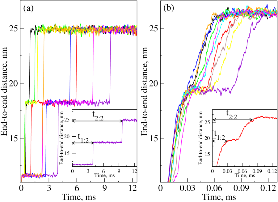
Figure 2: (Olga Kononova, Lee Jones, Valeri Barsegov)

Representative trajectories of the total end-to-end distance for the dimer $WW$$-$$WW$ obtained at $f$$=$$100pN$ and $f$$=$$160pN$ are compared in Fig. 2, which also shows graphically the definition of the first unfolding time $t_{1:2}$ and the second unfolding time $t_{2:2}$. We observe a typical “unfolding staircase”, i.e. a series of sudden step-wise increases in the end-to-end distance of $WW$$-$$WW$ as a function of time. These mark the consecutive unfolding transitions in $WW$ domains, which occur at the first unfolding time $t_{1:2}$ ($1$-st unfolding event) and at the second unfolding time $t_{2:2}$ ($2$-nd unfolding event). The unfolding transitions are more discrete at a lower force $f$$=$$100pN$ (Fig. 2a) but more continuous at a higher force $f$$=$$160pN$ (Fig. 2b). We remind that in experiment (but not in simulations), there is no way of knowing which domain has unfolded at any given time, and the time-ordered data ($t_{r:n}$) are the only observable quantities.

IV TOPOLOGICAL COUPLING AND MECHANICAL SYMMETRY BREAKING

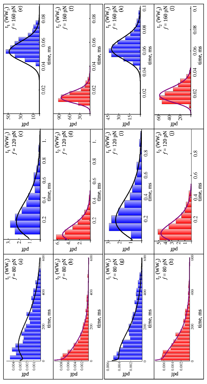
Figure 3: (Olga Kononova, Lee Jones, Valeri Barsegov)

To provide a basis for the Order statistics inference, we performed a direct statistical analysis of the simulaiton output for $WW$$-$$WW$ generated at $f$$=$$80$, $100$, $120$, $140$, and $160pN$ (parent data). The data sets contain $Q$$=$$1,000$ unfolding times for each force value and for each linker length. First, we constructed the histogram-based estimates of the unfolding times for the first domain ($WW_{1}$) and second domain ($WW_{2}$), which are compared in Fig. 3 (bin size was chosen using the Freedman-Diaconis rule Bura et al. (2009)). We calculated the average unfolding times $\mu_{1}^{T}$ and $\mu_{2}^{T}$ ($\mu_{i}^{T}$$=$$1/Q\sum_{j=1}^{Q}t_{ij}$, $i$$=$$1,2$), the standard deviations $\sigma_{1}^{T}$ and $\sigma_{2}^{T}$ ($\sigma_{i}$$=$$(E(t_{i}^{2})-(\mu_{i}^{T})^{2})^{1/2}$, where $E(t_{i}^{2})$ is the second moment of $t_{i}$, $i$$=$$1,2$), and the values of the skewness of distributions $\gamma_{1}^{T}$ and $\gamma_{2}^{T}$, and the Pearson correlation coefficient $\rho^{T}$$=$$\rho^{T}_{12}$. The skewness of the distributions was calculated using the formula $\gamma_{i}^{T}$$=$$(E(t_{i}^{3})-3\mu_{i}^{T}(\sigma_{i}^{T})^{2}-(\mu_{i}^{T})^{3})/(\sigma^{T}_{i})^{3}$, where $E(t_{i}^{3})$ is the third moment of $t_{i}$ ($i$$=$$1,2$). Pearson correlation coefficient was calculated as $\rho^{T}$$=$$(E(t_{1}t_{2})-\mu_{1}^{T}\mu_{2}^{T})/\sigma_{1}^{T}\sigma_{2}^{T}$, where $E(t_{1}t_{2})$ is the first moment of the product $t_{1}t_{2}$. These statistical measures are compared in Table I and II for the case of the linker of two and four residues, respectively.

The parent distributions of unfolding times are skewed, broadly distributed, and exponential-like at low forces ($f$$=$$80pN$) and become more narrowly distributed, and Gaussian-like at high forces ($f$$=$$160pN$; see Fig. 3). These changes become manifest when comparing the values of $\mu_{i}^{T}$, $\sigma_{i}^{T}$, and $\gamma_{i}^{T}$, $i$$=$$1,2$ (see Tables I and II). Here, $\mu_{1}^{T}$ and $\mu_{2}^{T}$ decrease as $f$ is increased, because the applied force destabilizes the native state of $WW$, and, hence, decreases their lifetimes. At low forces, dynamic fluctuations are not suppressed and the unfolding transitions are more variable (stochastic), which is reflected in the width of the distributions ($\sigma_{i}^{T}$). When $f$ is increased, fluctuations become less important and the unfolding events become increasingly more deterministic (less stochastic), which results in the decrease of $\sigma_{1}^{T}$ and $\sigma_{2}^{T}$.

Interestingly, we found that the unfolding times $t_{1}$ for the first domain ($WW_{1}$) and $t_{2}$ for the second domain ($WW_{2}$) are uncorrelated at low forces, but become correlated (dependent) at a high force ($f$$=$$160pN$). This is reflected in the values of the correlation coefficient $\rho^{T}$ (Table I and II). Hence, our results show that tension couples otherwise non-interacting protein domains forming a multi-domain protein. Because this result could have been observed in the case of physically interacting protein domains, e.g., through a common binding interface, we termed this effect the “topological coupling” to stress the importance of chain connectivity (topology). Hence, our results indicate that under large mechanical stress protein domains might become topologically coupled even in the absence of domain-domain interactions.

Another interesting finding is that although the unfolding times for the first domain $WW_{1}$ ($t_{1}$) and for the second domain $WW_{2}$ ($t_{2}$) are similarly distributed at a low force ($f$$=$$80pN$), these become more and more nonidenticaly distributed at higher forces ($f$$=$$100$$-$$160pN$). Indeed, the values of $\mu_{i}^{T}$, $\sigma_{i}^{T}$, and $\gamma_{i}^{T}$ for $i$$=$$1,2$ are very similar at $f$$=$$80pN$, yet, very different at $f$$=$$160pN$ (Tables I and II). Hence, our results indicate that increased tension breaks the mechanical symmetry. Indeed, identical protein domains $WW_{1}$ and $WW_{2}$ have very similar mechanical properties at a low force, but these become distinctly different at higher forces.

V FROM TIME-ORDERED DATA TO PARENT DISTRIBUTIONS

In force-clamp single-molecule experiments on multidomain proteins, experimentalists have no prior knowledge regarding the type of random variables measured. Our results for the dimer $WW$$-$$WW$ indicate that the mechanical force can topologically couple the non-interacting protein domains and can break the similarity in their physical properties even when domains are identical. Using our classification of random variables, the unfolding times for identical protein domains in a multi-domain protein might form a set of iid random variables at low forces, inid random variables at the intermediate force level, and dnid random variables at high enough forces. Hence, a unified approach is needed to analyze and model the different types of random variables. Here, we describe the results of application of Order statistics inference, developed in Section II, to characterize the forced unfolding times for the dimer $WW$$-$$WW$ obtained for different values of applied constant force $f$$=$$80$$-$$160pN$. The formalism adapted for the two-domain protein is presented in the Appendix.

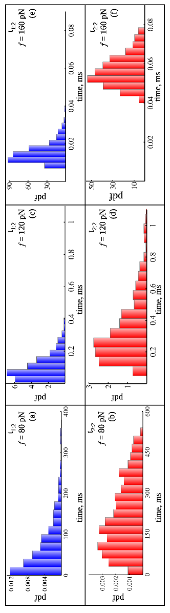
Figure 4: (Olga Kononova, Lee Jones, Valeri Barsegov)

Because in a single-molecule experiment size of the data sample might be small, we picked at random $330$ data points ($330$ pairs $(t_{1},t_{2})$) out of $Q$$=$$1,000$ observations from each data set. Next, we ordered the data for each pair to generate ordered unfolding times as observed in experiment. As an example for the dimer $WW$$-$$WW$ (linker of two residues), we present the histogram-based estimates of the pdf’s of the $1$-st unfolding time ($t_{1:2}$) and the $2$-nd unfolding time ($t_{2:2}$), obtained at $f$$=$$80$, $120$, and $160pN$ in Fig. 4. The histograms of the ordered unfolding times are markedly different in terms of their overall shape, width, and position of the maximum (most probable unfolding time). That the maximum for $t_{2:2}$ corresponds to longer times compared to the maximum for $t_{1:2}$ is not unexpected, since, by construction, $t_{1:2}$$<$$t_{2:2}$. A surprising element is that the histograms of $t_{2:2}$ have longer tais, which means that fluctuations play a more important role in the unfolding transitions that occur later in time. According to our formalism, the time-ordered data correspond to vectors of order statistics ${\bf T^{\prime}}$$=$$[t_{1:2},t_{2:2}]^{\dagger}$ described by the joint pdf $p_{{\bf T}^{\prime}}(t_{1:2},t_{2:2})$ (see Eq. (4)).

The model for two-domain protein $WW$$-$$WW$ has five unknown parameters: the average values $\mu_{1}$ and $\mu_{2}$, the standard deviations $\sigma_{11}$ and $\sigma_{22}$, and the covariance $\sigma_{12}$. These describe the statistics of vector ${\bf X}$$=$$[x_{1},x_{2}]^{\dagger}$. Once determined, they can be used to describe the parent statistics of vector ${\bf T}$$=$$[t_{1},t_{2}]^{\dagger}$. We employed the Maximum Likelihood Estimation (MLE) to obtain the vector of parameters, ${\bf\theta}$$=$$(\mu_{1},\mu_{2},\sigma_{11},\sigma_{22},\sigma_{12})$. The likelihood function for the pdf given by Eq. (4) is $L(\theta)$$=$$\prod_{j=1}^{330}p_{\bf T^{\prime}}(\{t_{1:n},t_{2:n}\}_{j}|{\bf\theta})$, but in the model calculations we used the log-likelihood function, $\log[L(\theta)]$$=$$\sum_{j=1}^{330}\log p_{\bf T^{\prime}}(\{t_{1:n},t_{2:n}\}_{j}|{\bf\theta})$, to obtain the values of $\mu_{1}$, $\mu_{2}$, $\sigma_{11}$, $\sigma_{22}$, and $\sigma_{12}$. These quantities and Eqs. (5), (6), (7), and (8) were then used to obtain the parent statistics: the average quantities $\mu_{1}^{T}$ and $\mu_{2}^{T}$, the standard deviations $\sigma_{1}^{T}$ and $\sigma_{2}^{T}$, the skewness coefficients $\gamma_{1}^{T}$ and $\gamma_{2}^{T}$, and the correlation coefficient $\rho^{T}$ (see Appendix). Finally, the closed-form expressions for the parent pdf’s of unfolding times $p_{1}(t)$ and $p_{2}(t)$ were obtained by integrating out $t_{2}$ and $t_{1}$, respectively, in Eq. (3) for the joint parent pdf:

$$p_{i}(t)=\frac{1}{\sigma_{ii}\sqrt{2\pi}}\cdot\frac{1}{2\sqrt{t}}\Bigl{[}\exp(-\frac{(\sqrt{t}-\mu_{i})^{2}}{2\sigma_{ii}^{2}})+\exp(-\frac{(\sqrt{t}+\mu_{i})^{2}}{2\sigma_{ii}^{2}}\Bigr{]}\text{, }i=1,2$$ (6)

Statistical measures of the parent unfolding times (parent statistics of vector ${\bf T}$$=$$[t_{1},t_{2}]^{\dagger}$), $\mu_{1}^{T}$, $\mu_{2}^{T}$, $\sigma_{1}^{T}$, $\sigma_{2}^{T}$, and $\rho^{T}$, obtained by applying Order statistics inference to the order-statistics data, are compared with the same quantities, obtained from a direct statistical analysis of the parent data, in Tables I and II. The theoretical curves of the parent distributions $p_{i}(t)$ ($i=1,2$), generated by substituting the values of $\mu_{1}$, $\mu_{2}$, $\sigma_{11}$ and $\sigma_{22}$ (statistics of vector ${\bf X}$$=$$[x_{1},x_{2}]^{\dagger}$) into Eq.(6), are overlaid in Fig. 3 with the histograms of the parent unfolding times.

We witness a very good agreement between the histogram-based estimates and theoretical curves of the pdf’s of the parent unfolding times for both domains $WW_{1}$ and $WW_{2}$ and for all force values $f$$=$$80$, $120$, and $160pN$ in terms of the overall shape and position of the maximum (Fig. 3). In agreement with simulations, our theory predicts that at high forces the second domain ($WW_{2}$), to which the force is applied (Fig. 1), unravels on a faster timescale compared to the first domain ($WW_{1}$). Hence, our theory captures the growing inequality of the time distributions for $WW_{1}$ and $WW_{2}$ at larger forces reflecting the mechanical symmetry breaking. Comparing the values of $\mu_{i}^{T}$, $\sigma_{i}^{T}$, $\gamma_{i}^{T}$, and $\rho^{T}$, obtained using Order statistics inference, with the “true” values of these quantities from a direct statistical analysis, we see that the agreement is nearly quantitative for $\mu_{i}^{T}$ and $\sigma_{i}^{T}$ and very good for $\gamma_{i}^{T}$ at low forces ($f$$=$$80pN$). At larger forces ($>$$100pN$), the agreement for $\mu_{i}^{T}$ and $\sigma_{i}^{T}$ is very good, yet, the agreement for $\gamma_{i}^{T}$ is more qualitative rather than quantitative. Importantly, Order statistics inference correctly captured the mutual independence of unfolding times ($t_{1}$ and $t_{2}$) at low forces, which is reflected in small values of Pearson correlation coefficient $\rho^{T}$ for $f$$<$$140pN$. Order statistics inference correctly predicts the emergence of topological interactions at higher forces (i.e. for $f$$=$$160pN$), for which the values of $\rho^{T}$ are in the $0.1$$-$$0.3$-range (Tables I and II).

VI DISCUSSION

Single-molecule force spectroscopy has enabled researchers to uncover the mechanism of adaptation of protein structures to mechanical loads $\breve{Z}$oldak and Rief (2013); Anthony et al. (2012). These experiments are now routinly used to study proteins and other biomolecules beyond the ensemble average picture and to map the entire distributions of the relevant molecular characteristics Barsegov and Mukamel (2002a, b). Yet, existing theoretical approaches for analyzing and modeling the experimental results lag behind. This calls for the development of next generation theoretical methods, which take into account both the complexity of the problem and the nature and statistics of experimental observables.

In the previos studies, we have demonstrated that the unfolding times observed in the constant force (force-clamp) measurements on a multidomain protein $D_{1}$$-$$D_{2}$$-$$\ldots$$-$$D_{n}$ comprize a set of the $r$-th order statistics, $t_{r:n}$ ($r$$=$$1,2,\ldots,n$) Bura et al. (2007a), and that the unfolding forces observed in the constant velocity (force-ramp) measurements form a set of the first order statistic $t_{1:n}$ in a sample of decreasing size ($n,n-1,\ldots,1$) Zhmurov et al. (2010a). We have also developed rigorous statistical tests for classification of random variables measured in these experiments Zhmurov et al. (2010a). Here, we developed an Order statistical theory to describe coupled proteins forming a multimeric protein or proteins forming the tertiary structure within the same multidomain protein subject to the mechanical stress. We focused on interesting new effects of tension-induced mechanical symmetry breaking and topological coupling in multi-domain proteins formed by the physically non-interacting protein domains, using an example of the two-domain protein $WW$$-$$WW$. However, our theory can also be used to characterize the physico-chemical properties of proteins with strong domain-domain interactions, such as fibrin fibers, microtubules, and actin filaments mentioned in the introduction. Strong interactions will translate into large values of the off-diagonal elements of the covariance matrix (Pearson correlation coefficient).

Our approach is based on Order statistics inference, which proved to be successful at solving the inverse problems. The approach can be used to accurately analyze, interpret, and model the results of protein forced unfolding measuremens available from the constant force assays on multimeric and multidomain proteins. One of the main results of this paper is that Order statistics inference enables one to analyze and model the forced unfolding times for a multi-domain protein formed by noninteracting identical domains (iid case) and non-identical domains (inid case), and by interacting identical domains (did case) and non-identical domains (dnid case). With little effort, the formalism can be extended to analyze the results of constant velocity measurements. We applied our approach to analyze the results of protein forced unfolding in silico for the dimer $WW$$-$$WW$ of the all-$\beta$-sheet $WW$ domains J$\ddot{a}$ger et al. (2001); Ferguson et al. (2003). In simulations, one can access “the parent data” and “the time-ordered data”. This was used to compare directly the various statistical measures - the distributions of unfolding times, the average unfolding times, the standard deviations, and the skeweness of the distributions, obtained from the statistical analysis of the parent unfolding times for domains $WW_{1}$ and $WW_{2}$, and the same measures, obtaineed by applying Order statistics inference to the time-ordered data. A very good agreement obtained between the statistics of unfolding times from pulling simulations and from the theoretical inference validates our theory. The presense of correlations is reflected in the inequality of the joint distribution to the product of the marginals, i.e. $p_{\bf T}(t_{1},t_{2})$$\neq$$p_{1}(t)$$p_{2}(t)$ Barsegov and Mukamel (2002a, b). In the bivariate case for just two domains, dynamic correlations between the parent unfolding times $t_{1}$ and $t_{2}$ are contained in the off-diagonal matrix element $\sigma_{12}^{T}$ of the covariance matrix ${\bf\Sigma}$ for vector ${\bf X}$$=$$[x_{1},x_{2}]^{\dagger}$. Order statistics inference correctly detected the absence of correlations at a small force ($f$$=$$80$, $100$ and $120pN$), and the presence of correlations at a large force ($f$$=$$160pN$).

We found the mechanical symmetry breaking and topological interactions observed in a multi-domain protein subject to tension. The growing asymmetry in the mechanical properties of otherwise identical protein domains comprising a multi-domain protein, can be understood by considering an example of $WW$$-$$WW$. When the pulling force is applied, it takes time $\tau_{f}$ for tension to propagate from the tagged residue in domain $WW_{2}$ to the other domain $WW_{1}$. Hence, domain $WW_{2}$ is subjected to the mechanical force for a longer time than domain $WW_{1}$ (Fig. 1). When force is large enough so that the average unfolding time $\mu_{f}$ becomes comparable with $\tau_{f}$, tension propagation prolongs the lifetime of the more distal domain $WW_{1}$, i.e. $\mu_{1}(f)$$\approx$$\mu_{f}$$+$$\tau_{f}$ versus $\mu_{2}(f)$$\approx$$\mu_{f}$. This is reflected in the inequality of the distributions of unfolding times for domains $WW_{1}$ and $WW_{2}$ (Fig. 3). But this same result would have been observed for a different two-domain protein, say $D_{1}$$-$$D_{2}$, formed by the non-identical domains, e.g., the mechanically stronger domain $D_{1}$ and mechanically weaker domain $D_{2}$, characterized by the differently distributed unfolding times.

The topological coupling can be understood using a concept of correlation length. In the folded state, overall bending flexibility is determined by the mobility at the domain-domain interface. Under low tension, the average inter-domain angle $\theta$ should show large deviations from the $180^{\circ}$-angle, $\Delta\theta$, and the correlation length $l_{c}$ is short. Under high tension, $\Delta\theta$ decreases and $l_{c}$ increases. This same result would have been observed for the domains that interact, e.g., through their inter-domain interface. Domain interactions would have decreased the mobility at the domain-domain interface, which, in turn, would have resulted in smaller $\Delta\theta$ and longer $l_{c}$. The averaged squared deviations of the inter-domain angle can be linked to the correlation length as $\langle\Delta\theta^{2}\rangle$$=$$2d/l_{c}$, where $d$ is the inter-domain distance. We estimated $l_{c}$ using the results of pulling simulations for $WW$$-$$WW$ (linker of two residues). For $f$$=$$100pN$, $d$$\approx$$1.2nm$ and $|\Delta\theta|$$\approx$$30^{\circ}$, and $l_{c}$$\approx$$1.8nm$ is shorter than the average size of the $WW$ domain at equilibrium ($\approx$$3$$-$$4nm$). For $f$$=$$160pN$, $d$$\approx$$2.8nm$ and $|\Delta\theta|$$\approx$$15^{\circ}$. This results in the three-fold increase in $l_{c}$$\approx$$5.2nm$, which now exceeds the dimension of $WW$ domain. Hence, under high tension $WW$ domains unravel in a concerted fasion, which is reflected in the dependence of the unfolding times $t_{1}$ and $t_{2}$ at large forces (Tables I and II).

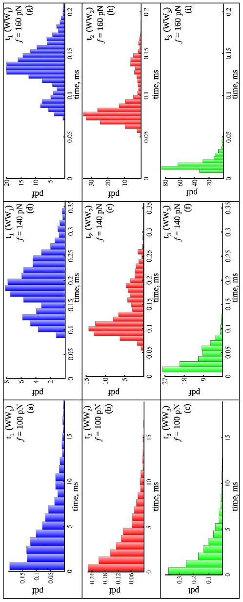
Figure 5: (Olga Kononova, Lee Jones, Valeri Barsegov)

To provide the reader with yet another glimpse of the hidden complexity underlying a seemingly trivial problem of unfolding of a multi-domain protein, we performed pulling simulations for the trimer $WW$$-$$WW$$-$$WW$, in which the force was applied to the third domain ($WW_{3}$). The histograms of unfolding times for the first domain $WW_{1}$ ($t_{1}$), second domain $WW_{2}$ ($t_{2}$), and third domain $WW_{3}$ ($t_{3}$) are compared in Fig. 5. Numerical values of the correlation coefficients for pair-wise correlations $\rho^{T}_{ij}$, $i$$\neq$$j$$=$$1,2,3$, of the unfolding times are summarized in Table III. We see that the distributions of unfolding times are nearly identical and unimodal, reflecting the mechanical symmetry, at a low $100pN$-force; yet, the time distributions become increasingly more different with the increasing tension. Indeed, the distributions of unfolding times for $WW_{1}$ and $WW_{2}$, but not for $WW_{2}$, develop the second mode at $f$$=$$140pN$. The parent unfolding times for $WW_{1}$ ($t_{1}$) and $WW_{2}$ ($t_{2}$), but not for $WW_{1}$ and $WW_{3}$ and not for $WW_{2}$ and $WW_{3}$, develop correlations, which tend to grow with force (Table III).

VII CONCLUSION

Intramolecular and intermolecular interactions involving proteins are at the core of virtually every biological process. Here, we developed and tested a new Order statistics approach for detecting and describing biomolecular interactions. Order statistics offers a new tool kit for accurate interpretation and modeling of experimental data on multidomain proteins, multimeric proteins, and engineered polyproteins available from single-molecule force spectroscopy. Looking into the future, we anticipate that Order statistics based calculus of probability will play an important role when single-molecule techniques will expand into new avenues of research such as folding of multi-domain proteins Wang et al. (2012), protein folding in cellular environment, and nanomechanics of protein assemblies (protein fibers, microtubules, actin filaments, viruses, etc.) Zhmurov et al. (2011a); Zhmurov et al. (2012). Also, life processes in living cells are coordinated both spatially and temporally. In this respect, Order statistics builds in causality into a theoretical description in a natural way.

Mechanical symmetry breaking and topological coupling might be related to the biological utility of proteins. The structural design of multidomain proteins - number of domains, linker length, etc., carves out a larger “parameter space” for the physical characteristics such as mechanical strength, tolerance to fluctuations, correlation length, all of which are force-dependent. As we showed in the paper, when tension is high enough, this design permits the “mechanical differentiation” of protein domains, which become, in some sense, “functional isoforms” of the same structural unit. Protein systems may have evolved to select certain modular architectures with the optimal physico-chemical properties for efficient mechanical integration of forces. Also, the mechanical stress promotes coupling between structural elements, which transforms a mechanically non-cooperative system into a highly cooperative one. This might be a mechanism of information transfer over long distances to coordinate cell processes over the relevant lengthscales and timescales Wang et al. (2009).

Acknowledgments: This work was supported by the American Heart Association (Grant 09SDG2460023) and by the Russian Ministry of Education and Science (Grant 14.A18.21.1239)

APPENDIX: ORDER STATISTICS INFERENCE FOR TWO-DOMAIN CASE

In the case of a two-domain protein $D_{1}$$-$$D_{2}$, the unfolding time data can be represented by vectors ${\bf T^{\prime}}$$=$$[t_{1:2},t_{2:2}]^{\dagger}$ containing the first and second order statistic. These data can be used to gather information about parent vectors ${\bf T}$$=$$[t_{1},t_{2}]^{\dagger}$ for the first domain ($D_{1}$) and second domain ($D_{2}$). For each vector ${\bf T}$ we define vector ${\bf X}^{2}$$=$$[x_{1}^{2},x_{2}^{2}]^{\dagger}$, in which random variables $x_{1}$ and $x_{2}$ are sampled from the Gaussian distribution (see Eq. (1)). Statistics of $x_{1}$ and $x_{2}$ are described by the vector of the average ${\bf\mu}$$=$$[\mu_{1},\mu_{2}]^{\dagger}$ and the covariance matrix ${\bf\Sigma}$$=$$\Bigl{[}\begin{smallmatrix}\sigma_{11}^{2}&\sigma_{12}\\ \sigma_{21}&\sigma_{22}^{2}\end{smallmatrix}\Bigr{]}$, where $\sigma_{11}^{2}$ and $\sigma_{22}^{2}$ are the variances of $x_{1}$ and $x_{2}$, respectively, and $\sigma_{12}$$=$$\sigma_{21}$ is the covariance. Eq. (3) for the joint pdf of the parent data ${\bf T}$$=$$[t_{1},t_{2}]^{\dagger}$ becomes

$$p_{{\bf T}}(t_{1},t_{2})=\frac{1}{2\pi\sqrt{|{\bf\Sigma}|}}\cdot\frac{1}{2^{2}\sqrt{t_{1}\cdot t_{2}}}\cdot\sum_{{\bf s}}{e^{-\frac{1}{2}({\bf s}{\bf\sqrt{T}}-{\bf\mu})^{\dagger}{\bf\Sigma}^{-1}({\bf s}{\bf\sqrt{T}}-{\bf\mu})}}$$ (1)

where $|{\bf\Sigma}|$$=$$\sigma_{11}^{2}\sigma_{22}^{2}$$-$$\sigma_{12}^{2}$ is the determinant and ${\bf\Sigma}^{-1}$$=$$\frac{1}{|{\bf\Sigma}|}\Bigl{[}\begin{smallmatrix}\sigma_{22}^{2}&-\sigma_{12}\\ -\sigma_{12}&\sigma_{11}^{2}\end{smallmatrix}\Bigr{]}$ is the inverse of the covariance matrix ${\bf\Sigma}$. In Eq. (1), ${\bf s}=[s_{1},s_{2}]^{\dagger}=\left\{[1,1]^{\dagger},[1,-1]^{\dagger},[-1,1]^{\dagger},[-1,-1]^{\dagger}\right\}$ are vectors of all possible signs of $\sqrt{t_{1}}$ and $\sqrt{t_{2}}$ and ${\bf s\sqrt{T}}$$=$$[s_{1}\sqrt{t_{1}},s_{2}\sqrt{t_{2}}]^{\dagger}$ is the vector of inverse values, which correspond to all possible branches of the inverse transformation $[t_{1},t_{2}]$$=$$[x_{1}^{2},x_{2}^{2}]$. Performing vector multiplication in the exponent of the exponential function forming the sum in Eq. (1), we obtain:

$$({\bf s}{\bf\sqrt{T}}-{\bf\mu})^{\dagger} {\bf\Sigma}^{-1} ({\bf s}{\bf\sqrt{T}}-{\bf\mu})$$ (2)

$$= \frac{(s_{1}\sqrt{t_{1}}-\mu_{1})^{2}\sigma_{22}^{2}+(s_{2}\sqrt{t_{2}}-\mu_{2})^{2}\sigma_{11}^{2}-2(s_{1}\sqrt{t_{1}}-\mu_{1})(s_{2}\sqrt{t_{2}}-\mu_{2})\sigma_{12}}{\sigma_{11}^{2}\sigma_{22}^{2}-\sigma_{12}^{2}}$$

which, depending on the choice of ${\bf s}$$=$$[s_{1},s_{2}]^{\dagger}$, takes the following form:

$$k_{1}(t_{1},t_{2})=\frac{(\sqrt{t_{1}}-\mu_{1})^{2}\sigma_{22}^{2}+(\sqrt{t_{2}}-\mu_{2})^{2}\sigma_{11}^{2}-2(\sqrt{t_{1}}-\mu_{1})(\sqrt{t_{2}}-\mu_{2})\sigma_{12}}{2(\sigma_{12}^{2}-\sigma_{11}^{2}\sigma_{22}^{2})}\text{, }{\bf s}=[1,1]^{\dagger}\\$$

$$k_{2}(t_{1},t_{2})=\frac{(\sqrt{t_{1}}-\mu_{1})^{2}\sigma_{22}^{2}+(\sqrt{t_{2}}+\mu_{2})^{2}\sigma_{11}^{2}+2(\sqrt{t_{1}}-\mu_{1})(\sqrt{t_{2}}+\mu_{2})\sigma_{12}}{2(\sigma_{12}^{2}-\sigma_{11}^{2}\sigma_{22}^{2})}\text{, }{\bf s}=[1,-1]^{\dagger}\\$$

$$k_{3}(t_{1},t_{2})=\frac{(\sqrt{t_{1}}+\mu_{1})^{2}\sigma_{22}^{2}+(\sqrt{t_{2}}-\mu_{2})^{2}\sigma_{11}^{2}+2(\sqrt{t_{1}}+\mu_{1})(\sqrt{t_{2}}-\mu_{2})\sigma_{12}}{2(\sigma_{12}^{2}-\sigma_{11}^{2}\sigma_{22}^{2})}\text{, }{\bf s}=[-1,1]^{\dagger}\\$$

$$k_{4}(t_{1},t_{2})=\frac{(\sqrt{t_{1}}+\mu_{1})^{2}\sigma_{22}^{2}+(\sqrt{t_{2}}+\mu_{2})^{2}\sigma_{11}^{2}-2(\sqrt{t_{1}}+\mu_{1})(\sqrt{t_{2}}+\mu_{2})\sigma_{12}}{2(\sigma_{12}^{2}-\sigma_{11}^{2}\sigma_{22}^{2})}\text{, }{\bf s}=[-1,-1]^{\dagger}\\$$

Substituting these expressions for $k_{j}$$=$$k_{j}(t_{1},t_{2})$ ($j$$=$$1,2,3,4$) and the expression for $|{\bf\Sigma}|$ in Eq. (1), we obtain the closed form expression for the joint pdf of the parent data:

$$p_{{\bf T}}(t_{1},t_{2})=\frac{1}{2\pi\sqrt{\sigma_{11}^{2}\sigma_{22}^{2}-\sigma_{12}^{2}}}\cdot\frac{1}{4\sqrt{t_{1}\cdot t_{2}}}\cdot\sum_{j=1}^{4}{e^{k_{j}(t_{1},t_{2})}}$$ (3)

in which the summation over ${\bf s}$ is replaced with the summation over $j$.

Next, to obtain the closed form expression for the joint pdf of the order statistics, we use Eq. (4) and take into account possible permutations of the vector components of order statistics $[t_{\kappa(1):2},t_{\kappa(2):2}]^{\dagger}$­. In the 2D-case, there are only two options, namely vector $[t_{1:2},t_{2:2}]^{\dagger}$­ and vector $[t_{2:2},t_{1:2}]^{\dagger}$­, which correspond to permutations $(t_{1},t_{2})$­ and $(t_{2},t_{1})$­ of the parent data. Then, the joint pdf of the order statistics is given by

$$p_{{\bf T^{\prime}}}(t_{1:2},t_{2:2}) = p_{{\bf T}}(t_{1},t_{2})+p_{{\bf T}}(t_{2},t_{1})$$ (4)

$$= \frac{1}{4\sqrt{t_{1}\cdot t_{2}}}\cdot\frac{1}{2\pi\sqrt{\sigma_{11}^{2}\sigma_{22}^{2}-\sigma_{12}^{2}}}$$

$$\times \Bigl{[}\exp(\frac{(\sqrt{t_{1}}-\mu_{1})^{2}\sigma_{22}^{2}+(\sqrt{t_{2}}-\mu_{2})^{2}\sigma_{11}^{2}-2(\sqrt{t_{1}}-\mu_{1})(\sqrt{t_{2}}-\mu_{2})\sigma_{12}}{2(\sigma_{12}^{2}-\sigma_{11}^{2}\sigma_{22}^{2})})$$

$$+ \exp(\frac{(\sqrt{t_{1}}-\mu_{1})^{2}\sigma_{22}^{2}+(\sqrt{t_{2}}+\mu_{2})^{2}\sigma_{11}^{2}+2(\sqrt{t_{1}}-\mu_{1})(\sqrt{t_{2}}+\mu_{2})\sigma_{12}}{2(\sigma_{12}^{2}-\sigma_{11}^{2}\sigma_{22}^{2})})$$

$$+ \exp(\frac{(\sqrt{t_{1}}+\mu_{1})^{2}\sigma_{22}^{2}+(\sqrt{t_{2}}-\mu_{2})^{2}\sigma_{11}^{2}+2(\sqrt{t_{1}}+\mu_{1})(\sqrt{t_{2}}-\mu_{2})\sigma_{12}}{2(\sigma_{12}^{2}-\sigma_{11}^{2}\sigma_{22}^{2})})$$

$$+ \exp(\frac{(\sqrt{t_{1}}+\mu_{1})^{2}\sigma_{22}^{2}+(\sqrt{t_{2}}+\mu_{2})^{2}\sigma_{11}^{2}-2(\sqrt{t_{1}}+\mu_{1})(\sqrt{t_{2}}+\mu_{2})\sigma_{12}}{2(\sigma_{12}^{2}-\sigma_{11}^{2}\sigma_{22}^{2})})$$

$$+ \exp(\frac{(\sqrt{t_{2}}-\mu_{1})^{2}\sigma_{22}^{2}+(\sqrt{t_{1}}-\mu_{2})^{2}\sigma_{11}^{2}-2(\sqrt{t_{2}}-\mu_{1})(\sqrt{t_{1}}-\mu_{2})\sigma_{12}}{2(\sigma_{12}^{2}-\sigma_{11}^{2}\sigma_{22}^{2})})$$

$$+ \exp(\frac{(\sqrt{t_{2}}-\mu_{1})^{2}\sigma_{22}^{2}+(\sqrt{t_{1}}+\mu_{2})^{2}\sigma_{11}^{2}+2(\sqrt{t_{2}}-\mu_{1})(\sqrt{t_{1}}+\mu_{2})\sigma_{12}}{2(\sigma_{12}^{2}-\sigma_{11}^{2}\sigma_{22}^{2})})$$

$$+ \exp(\frac{(\sqrt{t_{2}}+\mu_{1})^{2}\sigma_{22}^{2}+(\sqrt{t_{1}}-\mu_{2})^{2}\sigma_{11}^{2}+2(\sqrt{t_{2}}+\mu_{1})(\sqrt{t_{1}}-\mu_{2})\sigma_{12}}{2(\sigma_{12}^{2}-\sigma_{11}^{2}\sigma_{22}^{2})})$$

$$+ \exp(\frac{(\sqrt{t_{2}}+\mu_{1})^{2}\sigma_{22}^{2}+(\sqrt{t_{1}}+\mu_{2})^{2}\sigma_{11}^{2}-2(\sqrt{t_{2}}+\mu_{1})(\sqrt{t_{1}}+\mu_{2})\sigma_{12}}{2(\sigma_{12}^{2}-\sigma_{11}^{2}\sigma_{22}^{2})})\Bigr{]}$$

To obtain the average values $\mu_{1}$ and $\mu_{2}$, the standard deviations $\sigma_{11}$ and $\sigma_{22}$, and the covariance $\sigma_{12}$, we used the Maximum Likelihood Estimation method (Section V) and the joint pdf of the order statistics (see Eq. (4)). These parameters correspond to the vector ${\bf X}$$=$$[x_{1},x_{2}]^{\dagger}$, which allows us to estimate the average value ($\mu^{T}_{i}$), the standard deviation ($\sigma^{T}_{i}$), the skewness of the distribution ($\gamma^{T}_{i}$), and the correlation coefficient ($\rho^{T}$) for the parent data ${\bf T}$$=$$[t_{1},t_{2}]^{\dagger}$.

The theoretically estimated average unfolding times for domains $D_{1}$ and $D_{2}$ are given by

$$\mu^{T}_{i} = E(t_{i})=E(x_{i}^{2})$$ (5)

$$= \mu_{i}^{2}+\sigma_{ii}^{2},\quad i=1,2$$

where $E(t_{i})$ denotes the expected value of $t_{i}$ and $E(x_{i}^{2})$ is the second moment of $x_{i}$. The standard deviations are given by

$$\sigma^{T}_{i} = \sqrt{Var(t_{i})}=\sqrt{Var(x_{i}^{2})}$$ (6)

$$= \sqrt{E(x_{i}^{4})-(E(x_{i}^{2}))^{2}}$$

$$= \sqrt{4\sigma_{ii}^{2}\mu_{i}^{2}+2\sigma_{ii}^{4}},\quad i=1,2$$

where $Var(t_{i})$$=$$Var(x_{i}^{2})$ is the variance of the parent unfolding times $t_{i}$$=$$x_{i}^{2}$, and $E(x_{i}^{2})$ and $E(x_{i}^{4})$ are the second and fourth moments of $x_{i}$, respectively ($i$$=$$1,2$). The skewness of the distributions can be estimated as

$$\gamma^{T}_{i} = \frac{E(t_{i}^{3})-3\mu^{T}_{i}(\sigma^{T}_{i})^{2}-(\mu^{T}_{i})^{3}}{(\sigma^{T}_{i})^{3}}$$ (7)

$$= \frac{E(x_{i}^{6})-3\mu^{T}_{i}(\sigma^{T}_{i})^{2}-(\mu^{T}_{i})^{3}}{(\sigma^{T}_{i})^{3}}$$

$$= \frac{24\mu_{i}^{2}\sigma_{ii}^{4}+8\sigma_{ii}^{6}}{\sqrt{(4\sigma_{ii}^{2}\mu_{i}^{2}+2\sigma_{ii}^{4})^{3}}},\quad i=1,2$$

The correlation coefficient of unfolding times $t_{1}$ and $t_{2}$, $\rho^{T}$$=$$\rho_{ij}$ ($i$$\neq$$j$$=$$1,2$) is defined as

$$\rho^{T} = \frac{E(t_{1}t_{2})-E(t_{1})E(t_{2})}{\sqrt{Var(t_{1})}\sqrt{Var(t_{2})}}$$ (8)

$$= \frac{E(x_{1}^{2}x_{2}^{2})-E(x_{1}^{2})E(x_{2}^{2})}{\sqrt{Var(x_{1}^{2})}\sqrt{Var(x_{2}^{2})}}$$

In order to calculate $E(x_{1}^{2}x_{2}^{2})$ - the expected value of $x_{1}^{2}$ and $x_{2}^{2}$, we rewrite $x_{2}$ in the form $x_{2}=\mu_{2}+\rho\frac{\sigma_{22}}{\sigma_{11}}(x_{1}-\mu_{1})+\sigma_{22}\sqrt{1-\rho^{2}}R$, where $R$ is a normal random variable, independent of $x_{1}$, with zero mean and unit variance, and $\rho$ is the correlation coefficient for $x_{1}$ and $x_{2}$, given by $\rho=\sigma_{12}/(\sigma_{11}\sigma_{22})$. Then, $E(x_{1}^{2}x_{2}^{2})$ becomes $E(x_{1}^{2}x_{2}^{2})=E(x_{1}^{2}(\mu_{2}+\rho\frac{\sigma_{22}}{\sigma_{11}}(x_{1}-\mu_{1})+\sigma_{22}\sqrt{1-\rho^{2}}R)^{2})$. Simplifying the expression for $E(x_{1}^{2}x_{2}^{2})$ we obtain:

$$E(x_{1}^{2}x_{2}^{2})=A^{2}E(x_{1}^{2})+\frac{\sigma_{12}^{2}}{\sigma_{11}^{4}}E(x_{1}^{4})+2A\frac{\sigma_{12}}{\sigma_{11}^{2}}E(x_{1}^{3})+(\sigma_{22}^{2}-\frac{\sigma_{12}^{2}}{\sigma_{11}^{2}})E(x_{1}^{2})$$ (9)

where the coefficient $A$, the third moment $E(x_{1}^{3})$ of $x_{1}$, and the fourth moment $E(x_{1}^{4})$ of $x_{1}$ are given, respectively, by

$$A = \mu_{2}-\frac{\sigma_{12}}{\sigma_{11}^{2}}\mu_{1},$$

$$E(x_{1}^{3}) = \mu_{1}^{3}+3\mu_{1}\sigma_{11}^{2},$$

$$E(x_{1}^{4}) = \mu_{1}^{4}+6\mu_{1}^{2}\sigma_{11}^{2}+3\sigma_{11}^{4}$$ (10)

The correlation coefficient for the parent data can be calculated theoretically by substituting Eqs. (APPENDIX: ORDER STATISTICS INFERENCE FOR TWO-DOMAIN CASE) into Eq. (9), then substituting Eq. (9) into the second line in Eq. (8), and finally using Eqs. (5) and (6) for the average unfolding time $\mu_{i}^{T}$$=$$E(x_{i}^{2})$ and the variance $\sigma_{i}^{T}$$=$$\sqrt{Var(x_{i}^{2})}$ ($i$$=$$1,2$).

FIGURE CAPTIONS

Figure 1: Schematic representation of the native structure of dimer $WW$$-$$WW$, formed by the C-terminal to N-terminal connected all-$\beta$-sheet $WW$ domains (PDB code: 1PIN). The first $WW$ domain, denoted as $WW_{1}$, is shown in blue, the second $WW$ domain, denoted as $WW_{2}$, is shown in red, and the two-residue linker is shown in yellow color. In pulling simulations, the constant force $f$ is applied to the C-terminus of domain $WW_{2}$ in the direction coinsiding with the end-to-end vector of dimer $WW$$-$$WW$; the N-terminus of domain $WW_{1}$ is constrained. Structural analysis of unfolding trajectories revealed that the force unfolding transitions from the native folded state ($F$) to the unfolded state ($U$) in each $WW$ domain occur in a single step, $F$$\to$$U$. Shown are the two possible scenarios. In the first pathway (left), $WW_{1}$ unfolds first ($1$-st unfolding time $t_{1:2}$) and $WW_{2}$ unfolds second ($2$-nd unfolding time $t_{2:2}$). In the second pathway (right), $WW_{1}$ unfolds second ($t_{2:2}$) and $WW_{2}$ unfolds first ($t_{1:2}$).

Figure 2: The time-evolution of the end-to-end distance of the dimer $WW$$-$$WW$ (see Fig. 1), $Y$, under the influence of constant pulling force of $f$$=$$100pN$ (panel $a$) and $f$$=$$160pN$ (panel $b$). Shown in different color are a few representative trajectories. The unfolding transitions in $WW$$-$$WW$ are reflected in the stepwise increases in $Y$, which occur at the $1$-st unfolding time $t_{1:2}$ (unfolding of $WW_{1}$ or $WW_{2}$), and $2$-nd unfolding time $t_{2:2}$ (unfolding of $WW_{1}$ or $WW_{2}$). These transitions are magnified in the insets for each force value for just one simulation run.

Figure 3: The “parent unfolding times” $t_{i}$, $i$$=$$1,2$, for the dimer $WW$$-$$WW$ of domains $WW_{1}$ and $WW_{2}$ connected by the two-residue linker (panels $a$$-$$f$) and four-residue linker (panels $g$$-$$l$). Shown are the histogram-based estimates of the pdf’s of unfolding times for the first domain $WW_{1}$ ($t_{1}$, blue bars) and for the second domain $WW_{2}$ ($t_{2}$, red bars), obtained directly from the simulation output. These are compared with the theoretical curves of the same quantities obtained by applying Order statistics inference (black curves) for $f$$=$$80pN$ (panels $a$, $b$ and $g$, $h$), $f$$=$$120pN$ (panels $c$, $d$ and $i$, $j$), and $f$$=$$160pN$ (panels $e$, $f$ and $k$, $l$).

Figure 4: The “time-ordered unfolding times” $t_{r:2}$, $r$$=$$1,2$ for the dimer $WW$$-$$WW$ (two-residue linker). The data are represented by the histogram-based estimates of the pdf’s of the $1$-st unfolding time ($t_{1:2}$) and $2$-nd unfolding time ($t_{2:2}$) compared for $f$$=$$80pN$ (panels $a$ and $b$), $f$$=$$120pN$ (panels $c$ and $d$), and $f$$=$$160pN$ (panels $e$ and $f$).

Figure 5: The “parent unfolding times” $t_{i}$, $i$$=$$1,2$ and $3$, for the trimer $WW$$-$$WW$$-$$WW$ of $WW$ domains connected by linkers of two residues. Compared are the histogram-based estimates of the parent pdf’s of unfolding times for the first domain $WW_{1}$ ($t_{1}$, blue bars), second domain $WW_{2}$ ($t_{2}$, red bars), and third domain $WW_{3}$ ($t_{3}$, green bars), obtained directly from the simulation output generated for $f$$=$$100pN$ (panels $a$, $b$, and $c$), $f$$=$$140pN$ (panels $d$, $e$, and $f$), and $f$$=$$160pN$ (panels $g$, $h$, and $i$).

Table I: Statistical measures of the parent unfolding times for the first domain $WW_{1}$ ($t_{1}$), and second domain $WW_{2}$ ($t_{2}$), connected in the dimer $WW$$-$$WW$ by the two-residue linker: the average unfolding times $\mu^{T}_{1}$ and $\mu^{T}_{2}$, the standard deviations $\sigma^{T}_{1}$ and $\sigma^{T}_{2}$, the skewness of the distributions $\gamma^{T}_{1}$ and $\gamma^{T}_{2}$, the Pearson correlation coefficient $\rho^{T}$$=$$\rho_{12}^{T}$, and Spearman rank correlation coefficient $s^{T}$$=$$s_{12}^{T}$. The estimates of these measures (except for $s^{T}$), obtained directly from the simulation output, are compared with the estimates obtained by applying Order statistics inference (shown in parentheses).

Force,	$\mu^{T}_{1}$,	$\mu^{T}_{2}$,	$\sigma^{T}_{1}$,	$\sigma^{T}_{2}$,	$\gamma^{T}_{1}$	$\gamma^{T}_{2}$	$\rho^{T}$	$s^{T}$
pN	ms	ms	ms	ms
80	174.2	106.1	134.4	102.3	1.69	1.51	-0.012	0.006
	(189.8)	(93.5)	(143.7)	(88.5)	(1.2)	(1.55)	(-0.097)
100	4.13	2.25	3.60	2.25	1.41	1.67	-5$\cdot 10^{-5}$	0.025
	(4.19)	(2.09)	(3.77)	(1.87)	(1.46)	(1.67)	(-0.067)
120	0.32	0.13	0.23	0.12	1.71	1.98	-0.064	-0.049
	(0.31)	(0.13)	(0.23)	(0.08)	(1.20)	(0.98)	(-0.111)
140	0.093	0.034	0.031	0.019	1.21	2.01	0.014	0.132
	(0.095)	(0.032)	(0.024)	(0.016)	(0.39)	(0.76)	(0.174)
160	0.058	0.016	0.010	0.006	1.18	1.86	0.131	0.123
	(0.057)	(0.016)	(0.009)	(0.005)	(0.24)	(0.51)	(0.151)

Table II: Same quantities as in Table I but for the dimer $WW$$-$$WW$ of $WW$ domains connected by the linker of four residues.

Force,	$\mu^{T}_{1}$,	$\mu^{T}_{2}$,	$\sigma^{T}_{1}$,	$\sigma^{T}_{2}$,	$\gamma^{T}_{1}$	$\gamma^{T}_{2}$	$\rho^{T}$	$s^{T}$
pN	ms	ms	ms	ms
80	166.0	112.9	133.5	99.6	1.74	1.35	0.028	0.037
	(150.0)	(103.8)	(125.4)	(94.3)	(1.34)	(1.47)	(0.077)
100	3.80	2.46	3.30	2.30	1.42	1.62	0.030	0.052
	(4.04)	(2.52)	(3.59)	(1.97)	(1.44)	(1.24)	(0.048)
120	0.32	0.15	0.23	0.12	1.68	1.73	-0.026	-0.033
	(0.30)	(0.16)	(0.23)	(0.10)	(1.20)	(0.96)	(-0.004)
140	0.10	0.040	0.036	0.023	1.42	1.55	-0.017	0.069
	(0.10)	(0.039)	(0.032)	(0.021)	(0.46)	(0.83)	(-0.266)
160	0.065	0.021	0.011	0.008	1.19	1.00	0.259	0.255
	(0.064)	(0.021)	(0.011)	(0.008)	(0.25)	(0.55)	(0.285)

Table III: The Pearson correlation coefficients, $\rho^{T}_{ij}=\rho_{12}^{T}$, $\rho_{13}^{T}$, and $\rho_{22}^{T}$, and the Spearman rank correlation coeficients, $s^{T}_{ij}=s_{12}^{T}$, $s_{13}^{T}$, and $s_{22}^{T}$, quantifying the degree of pairwise correlations (dependence) of the parent unfolding times $t_{i}$ ($i$$=$$1,2,3$) for the first domain $WW_{1}$ ($t_{1}$), second domain $WW_{2}$ ($t_{2}$), and third domain $WW_{3}$ ($t_{3}$). These measures are obtained by performing a statistical analysis of the simulation output for the trimer $WW$$-$$WW$$-$$WW$ of $WW$ domains connected by the linkers of two residues.

Force, pN	$\rho_{12}^{T}$($s_{12}^{T}$)	$\rho_{13}^{T}$($s_{13}^{T}$)	$\rho_{23}^{T}$($s_{23}^{T}$)
100	-0.023 (0.032)	0.053 (0.050)	0.038 (0.035)
120	-0.073 (-0.130)	-0.035 (-0.039)	0.054 (-0.032)
140	-0.341 (-0.295)	0.042 (0.057)	0.043 (0.092)
160	-0.537 (-0.139)	0.038 (0.021)	-0.016 (-0.032)

References

- Puchner and Gaub (2009) E. M. Puchner and H. E. Gaub, Curr. Opin. Struct. Biol. 19, 605 (2009).
- Gautel (2011) M. Gautel, Curr. Opin. Cell. Biol. 23, 39 (2011).
- Kasza and Zallen (2011) K. E. Kasza and J. A. Zallen, Curr. Opin. Cell. Biol. 23, 30 (2011).
- Rodger P (2002) M. Rodger P, Curr. Opin. Cell. Biol. 14, 581 (2002).
- Nakamura et al. (2011) F. Nakamura, T. P. Stossel, and J. H. Hartwig, Cell. Adh. Migr. 5, 160 (2011).
- Tskhovrebova and Trinick (2010) L. Tskhovrebova and J. Trinick, J. Biomed. Biotechnol. 2010, 612482 (2010).
- Weisel (2008) J. W. Weisel, Science 320, 456 (2008).
- Leckband and Sivasankar (2012) D. Leckband and S. Sivasankar, Curr. Opin. Cell. Biol. 24, 620 (2012).
- Ramage (2012) L. Ramage, Cell Health Cytoskelet. 4, 1 (2012).
- Wang et al. (2009) N. Wang, J. D. Tytell, and D. E. Ingber, Nat. Rev. Mol. Cell. Bio. 10, 75 (2009).
- Brown et al. (2009) A. E. X. Brown, R. I. Litvinov, D. E. Discher, P. Purohit, and J. W. Weisel, Science 325, 741 (2009).
- Speir et al. (1995) J. A. Speir, S. Munshi, G. Wang, T. S. Baker, and J. E. Johnson, Structure 3, 63 (1995).
- Singh et al. (2010) P. Singh, C. Carraher, and J. E. Schwarzbauer, Annu. Rev. Cell Dev. Biol. 26, 397 (2010).
- Roos et al. (2010) W. H. Roos, R. Bruinsma, and G. J. L. Wuite, Nat. Phys. 6, 733 (2010).
- Lieleg et al. (2010) O. Lieleg, M. M. A. E. Claessens, and A. R. Bausch, Soft Matter 6, 218 (2010).
- Sutherland-Smith (2011) A. J. Sutherland-Smith, Biophys. Rev. 3, 15 (2011).
- Hertig and Vogel (2012) S. Hertig and V. Vogel, Curr. Biol. 22, R823 (2012).
- Barsegov and Thirumalai (2006) V. Barsegov and D. Thirumalai, J. Phys. Chem. 110, 26403 (2006).
- oldak and Rief (2013) G. oldak and M. Rief, Curr. Opin. Struct. Biol. 23, 48 (2013).
- Lannon et al. (2012) H. Lannon, E. Vanden-Eijnden, and J. Brujic, Biophys. J. 103, 2215 (2012).
- Fazal and Block (2011) F. M. Fazal and S. M. Block, Nat. Photonics 5, 318 (2011).
- Litvinov et al. (2012) R. I. Litvinov, A. Mekler, H. Shuman, J. S. Bennett, V. Barsegov, and J. W. Weisel, J. Biol. Chem. 287, 35272 (2012).
- Gumbel (2004) E. J. Gumbel, Statistics of Extremes (Dover Publications, New York, 2004).
- David and Nagaraja (2003) H. A. David and H. N. Nagaraja, Order Statistics (Willey Interscience, New York, 2003).
- Bura et al. (2007a) E. Bura, D. K. Klimov, and V. Barsegov, Biophys. J. 93, 1100 (2007a).
- Bura et al. (2007b) E. Bura, D. K. Klimov, and V. Barsegov, Biophys. J. 94, 2516 (2007b).
- Zhmurov et al. (2010a) A. Zhmurov, R. I. Dima, and V. Barsegov, Biophys. J. 99, 1959 (2010a).
- Jones (2013) L. K. Jones, Oper. Res. (2013), submitted.
- Jones and Larson (1995) L. Jones and R. C. Larson, O. R. S. A. J. Comput. 1, 89 (1995).
- Larson (1990) R. C. Larson, Manage. Sci. 36, 586 (1990).
- Zhmurov et al. (2011a) A. Zhmurov, A. E. X. Brown, R. I. Litvinov, R. I. Dima, J. W. Weisel, and V. Barsegov, Structure 19, 1615 (2011a).
- Zhmurov et al. (2012) A. Zhmurov, O. Kononova, R. I. Litvinov, R. I. Dima, V. Barsegov, and J. W. Weisel, J. Am. Chem. Soc. 134, 20396 (2012).
- Theisen et al. (2012) K. E. Theisen, A. Zhmurov, M. E. Newberry, V. Barsegov, and R. I. Dima, J. Phys. Chem. B 116, 8546 (2012).
- Duan et al. (2011) L. Duan, A. Zhmurov, V. Barsegov, and R. I. Dima, J. Phys. Chem. B 115, 10133 (2011).
- Hyeon et al. (2006) C. Hyeon, R. I. Dima, and D. Thirumalai, Structure 14, 1633 (2006).
- Koepf et al. (1999) E. K. Koepf, H. M. Petrassi, M. Sudol, and J. W. Kelly, Protein Sci. 8, 841 (1999).
- Veitshans et al. (1997) T. Veitshans, D. K. Klimov, and D. Thirumalai, Fold. Des. 2, 1 (1997).
- Zhmurov et al. (2010b) A. Zhmurov, R. I. Dima, Y. Kholodov, and V. Barsegov, Proteins 78, 2984 (2010b).
- Zhmurov et al. (2011b) A. Zhmurov, K. Rybnikov, Y. Kholodov, and V. Barsegov, J. Phys. Chem. B 115, 5278 (2011b).
- Bura et al. (2009) E. Bura, A. Zhmurov, and V. Barsegov, J. Chem. Phys. 130, 015102 (2009).
- Anthony et al. (2012) P. C. Anthony, C. F. Perez, C. Garcia-Garcia, and S. M. Block, Proc. Natl. Acad. Sci. USA 109, 1485 (2012).
- Barsegov and Mukamel (2002a) V. Barsegov and S. Mukamel, J. Chem. Phys. 117, 9465 (2002a).
- Barsegov and Mukamel (2002b) V. Barsegov and S. Mukamel, J. Chem. Phys. 116, 9802 (2002b).
- Jger et al. (2001) M. Jger, H. Nguyen, J. C. Crane, J. W. Kelly, and M. Gruebele, J. Mol. Biol. 311, 373 (2001).
- Ferguson et al. (2003) N. Ferguson, J. Berriman, M. Petrovich, T. D. Sharpe, J. T. Finch, and A. R. Fersht, Proc. Natl. Acad. Sci. USA 100, 9814 (2003).
- Wang et al. (2012) Y. Wang, X. Chu, Z. Suo, E. Wang, and J. Wang, J. Am. Chem. Soc. 134, 13755 (2012).