Structure and Stability of Filamentary Clouds Supported by Lateral Magnetic Field

Abstract

We have constructed two types of analytical models for an isothermal filamentary cloud supported mainly by magnetic tension. The first one describes an isolated cloud while the second considers filamentary clouds spaced periodically. Both the models assume that the filamentary clouds are highly flattened. The former is proved to be the asymptotic limit of the latter in which each filamentary cloud is much thinner than the distance to the neighboring filaments. We show that these models reproduce main features of the 2D equilibrium model of Tomisaka (2014) for filamentary cloud threaded by perpendicular magnetic field. It is also shown that the critical mass to flux ratio is $M/\Phi=(2\pi\sqrt{G})^{-1}$, where $M$, $\Phi$ and $G$ denote the cloud mass, the total magnetic flux of the cloud, and the gravitational constant, respectively. This upper bound coincides with that for an axisymmetric cloud supported by poloidal magnetic fields. We applied the variational principle for studying the Jeans instability of the first model. Our model cloud is unstable against fragmentation as well as the filamentary clouds threaded by longitudinal magnetic field. The fastest growing mode has a wavelength several times longer than the cloud diameter. The second model describes quasi-static evolution of filamentary molecular cloud by ambipolar diffusion.

1 Introduction

Interstellar magnetic field plays significant roles on the dynamics of molecular clouds. Magnetic field supports molecular cloud against gravitational collapse if it is strong enough. It is well known that the mass to flux ratio, i.e., the amount of gas contained in a magnetic flux tube, is the key parameter for the magnetic support. Mestel & Spitzer (1956) pointed out from the viral analysis that magnetic force reduces gravity by a constant factor independent of the size of the cloud. They evaluated the critical magnetic flux to support a cloud of mass, $M$, to be $\Phi_{c}=\pi\sqrt{G}M$ (Mestel & Paris, 1984). The virial theorem provides the correct scaling law but not quantitatively correct value for the critical mass. One needs equilibrium models to evaluate the critical value. Mouschovias (1976a, b) for the first time obtained a magnetohydrostatic equilibrium for a disk like cloud supported in part by magnetic field. He evaluated magnetic pressure and tension as well as self-gravity and gas pressure consistently. He confirmed that the mass to flux ratio is one of the key parameters. He also noticed that the equilibrium depends also on ratio of the magnetic pressure to the gas pressure and the flux function, i.e., the amount of gas contained in each magnetic flux. Tomisaka, Ikeuchi & Nakamura (1988) obtained a fitting formula for the critical equilibrium from their numerical results. It reads $\Phi_{c}=(0.17)^{-1}M\sqrt{G}\simeq 2\pi\sqrt{G}M$. Finite electrical conductivity changes the flux function through ambipolar diffusion and induces quasi-static contraction. When the magnetic field is weaker than the critical one, the gravitational collapse continues to form stars. Thus magnetohydrostatic equilibria help our understanding of the gravitational collapse to form stars.

Magnetohydrostatic equilibria depend on the configuration. We need to consider filamentary clouds in magnetohydrostatic equilibria since observed molecular clouds are often filamentary and associated with either longitudinal or perpendicular magnetic field. The magnetic field is parallel to elongation of the molecular cloud in the Ophiuchus star forming region while it is perpendicular in the Taurus (see, e.g., Moneti et al., 1984; Goodman et al, 1990; Palmeirim et al., 2013) and in the Musca (Pereyra & Magahães, 2004).

Stodółkiewcz (1963) and Ostriker (1964) obtained equilibrium model having the density distribution,

$$\rho(r) = \rho_{c}\left(1+\frac{r^{2}}{8H^{2}}\right)^{-2},$$ (1)

$$H^{2} = \frac{c_{s}^{2}}{4\pi G\rho_{c}},$$ (2)

for an isothermal filamentary cloud in the cylindrical coordinate, ($r,\varphi,z$), where $c_{s}$ and $G$ denote the isothermal sound speed and gravitational constant, respectively. Interestingly, the line density defined by

$$\lambda \equiv \int_{0}^{\infty}2\pi r\rho(r)dr=\frac{2c_{s}^{2}}{G},$$ (3)

does not depend on the filament width, $H$. Thus, this model is neutrally stable against radial contraction.

Stodółkiewcz (1963) showed that filamentary clouds having a larger line density can be sustained by purely longitudinal or partially helical magnetic field. These models are unstable against fragmentation, i.e., sinusoidal perturbation in the $z$-direction (see, e.g., Hanawa et al., 1993). The fragmentation and its further evolution were studied extensively by Tomisaka (1995), Nakamura et al. (1995) and others.

On the contrary, filamentary clouds permeated by magnetic field perpendicular to the axis have been studied little. Its structure was obtained only recently by Tomisaka (2014) referred to Paper I in the following. This is mainly because the structure is obtained only by extensive numerical computation solving the Poisson and Grad-Shafranov equations simultaneously. The latter is highly nonlinear since it describes force balance in the directions parallel and perpendicular to the magnetic field. It requires high spatial resolution especially when the filamentary cloud is condensed. Paper I showed that the maximum line density increases in proportion to the magnetic flux. In this paper we show analytical models which reproduce the main features of the 2D models obtained in Paper I.

When the line density is higher than $2c_{s}^{2}/G$ and thus supported mainly by magnetic field, the filamentary cloud is flattened like Italian pasta fettucine. The magnetic force is dominated by the magnetic tension. Then we can use the thin disk approximation to analyze the structure and stability of filamentary cloud permeated by perpendicular magnetic field.

This paper is organized as follows. In §2 we derive an analytical model for an isolated filamentary cloud. The mass to flux ratio is uniform in the model. In §3 we use the Fourier series for filamentary clouds arranged periodically. It is shown that the solution approaches to that obtained in §2 when the filament thickness is much smaller than the distance to the neighboring filaments. It is also shown that the ratio of the thickness to the distance can be regarded as the model parameter specifying the quasi-static evolution. In §4 we confirm that our 1D models reproduce the main features of the 2D model obtained in Paper I. In §5 the model obtained in §2 is proved to be unstable against fragmentation. In §6 we discuss the stability of the models obtained in §3.

2 Equilibrium Model

In this paper, we consider an isothermal flattened filamentary cloud having infinite length and infinitesimal thickness. This simplification is justified for observed filamentary clouds since their lengths are much larger than the widths and the magnetic fields are often perpendicular to cloud elongation on the sky. It is well known that self-gravitating clouds are flattened in the direction perpendicular to the global magnetic field. In the following we use the Cartesian coordinates in which the cloud is confined in the plane of $z=0$ and elongated in the $y$-direction. Both the gas and magnetic fields are uniform in the $y$-direction.

From the above assumptions we can express the gas density distribution as

$$\rho = \Sigma(x)\,\delta(z),$$ (4)

where $\Sigma(x)$ and $\delta(z)$ denote the surface density and the Dirac’s delta function, respectively. The Poisson equation reduces to

$$\left(\frac{\partial^{2}}{\partial x^{2}}+\frac{\partial^{2}}{\partial z^{2}}\right)\phi = 4\pi G\Sigma(x)\delta(z).$$ (5)

We obtain the boundary condition,

$$\left.\frac{\partial\phi}{\partial z}\right|_{z=+\varepsilon} = -\left.\frac{\partial\phi}{\partial z}\right|_{z=-\varepsilon}=2\pi G\Sigma(x).$$ (6)

by integrating Equation (5) in the vertical direction over the infinitesimal interval around $z=0$ (see, e.g., Binney & Tremaine, 2008, for the derivation). The symbol, $\varepsilon$, denotes an infinitesimally small positive quantity. The gravity is given by

$$g_{x} = -\frac{\partial\phi}{\partial x},$$ (7)

$$g_{z} = -\frac{\partial\phi}{\partial z}.$$ (8)

We assume for simplicity that the magnetic field has only the $x$- and $z$-components in the equilibrium. The condition for magneto-hydrostatic equilibrium requires that the magnetic field should be force free and hence current free outside the disk,

$$\frac{\partial B_{x}}{\partial z}-\frac{\partial B_{z}}{\partial x} = \frac{4\pi J_{y}(x)}{c}\delta(z),$$ (9)

since both the gravity and pressure thereof are negligibly small. The symbols, $c$ and $J_{y}(x)$, denote the speed of light and the electric surface current running in the $y$-direction inside the cloud per unit length in the $x$-direction, respectively. The magnetic field is kinked on the disk,

$$B_{x}(x,z=+\varepsilon) = -B_{x}(x,z=-\varepsilon)=\frac{2\pi J_{y}(x)}{c}.$$ (10)

Note that the gravity and magnetic field can be perfectly aligned outside the cloud. Both of them are divergence and rotation free, i.e., $\mbox{\boldmath$\nabla$}\cdot\mbox{\boldmath$g$}=0$, $\mbox{\boldmath$\nabla$}\times\mbox{\boldmath$g$}=0$, $\mbox{\boldmath$\nabla$}\cdot\mbox{\boldmath$B$}=0$, and $\mbox{\boldmath$\nabla$}\times\mbox{\boldmath$B$}=0$, outside the cloud, $z\neq 0$. In the following we focus on the case that the magnetic field is proportional to the gravity,

$$B_{x} = -\frac{\alpha}{\sqrt{G}}g_{x},$$ (11)

$$B_{z} = -\frac{\alpha}{\sqrt{G}}g_{z},$$ (12)

in $z>0$ and

$$B_{x} = \frac{\alpha}{\sqrt{G}}g_{x},$$ (13)

$$B_{z} = \frac{\alpha}{\sqrt{G}}g_{z},$$ (14)

in $z<0$, where $\alpha$ denotes a non-dimensional constant. This assumption is equivalent to the constant mass to flux ratio (isopedic in the terminology of Shu & Li, 1997),

$$\alpha = \frac{B_{z}(x,z=0)}{2\pi\sqrt{G}\Sigma(x)},$$ (15)

thanks to Equation (6). Hence, the cloud is subcritical (supercritical) when $\alpha>1$ ($\alpha<1$). When the mass to flux ratio is constant, the magnetic tension working on the cloud is proportional to the gravity,

$$\int_{-\varepsilon}^{+\varepsilon}\frac{\partial}{\partial z}\left(\frac{B_{x}B_{z}}{4\pi}\right)dz = \left.\frac{B_{x}B_{z}}{2\pi}\right|_{z=+\varepsilon}$$ (16)

$$= -\alpha^{2}g_{x}\Sigma,$$ (17)

in the cloud.

Equations (17) simplifies the equation for magnetohydrostatic balance in the $x$-direction,

$$\frac{\partial}{\partial x}\left(c_{s}^{2}\rho\right)+\frac{\partial}{\partial x}\left(\frac{B_{x}^{2}+B_{z}^{2}}{8\pi}\right)-\frac{\partial}{\partial z}\left(\frac{B_{x}B_{z}}{4\pi}\right) = g_{x}\rho,$$ (18)

where $c_{s}$ denotes the isothermal sound speed. Substituting Equation (17) into Equation (18) integrated over the infinitesimal interval around $z=0$, we obtain

$$\left(1-\alpha^{2}\right)g_{x}\Sigma+c_{s}^{2}\frac{\partial\Sigma}{\partial x} = 0.$$ (19)

The magnetic field reduces the effective gravity by a factor $\left(1-\alpha^{2}\right)$. See Shu & Li (1997) for the validity of this approximation. Equation (19) indicates that the cloud is in equilibrium only when $\alpha<1$ (supercritical).

In the following we consider the Lorentz profile,

$$\Sigma=\frac{\lambda}{\pi}\frac{a}{x^{2}+a^{2}}$$ (20)

as a model for the flattened filamentary cloud. The line density and FWHM of this model cloud are $\lambda$ and $2a$, respectively. Using the method of images we obtain the corresponding gravity,

$$\mbox{\boldmath$g$}=\left(\begin{array}[]{c}g_{x}\\ g_{z}\end{array}\right) = -\frac{z}{|z|}\frac{2G\lambda}{x^{2}+(|z|+a)^{2}}\left(\begin{array}[]{c}x\\ \displaystyle|z|+a\end{array}\right).$$ (25)

The pressure force is given by

$$c_{s}^{2}\frac{d\Sigma}{dx} = -\frac{2ac_{s}^{2}\lambda x}{\pi\left[x^{2}+(|z|+a)^{2}\right]^{2}}.$$ (26)

We obtain the condition for the magnetohydrostatic equilibrium,

$$G\lambda\left(1-\alpha^{2}\right)-c_{s}^{2} = 0,$$ (27)

by substituting Equations (20) through (26) to Equation (19). Equation (27) is rewritten as

$$\lambda=\frac{c_{s}^{2}}{2G}+\sqrt{\displaystyle\left(\frac{\Phi}{2\pi\sqrt{G}}\right)^{2}+\left(\frac{c_{s}^{2}}{2G}\right)^{2}},$$ (28)

by the help of Equation (15). When Equation (28) holds, the model cloud settles in an equilibrium for any $a$. In other words, the width of the cloud is not specified by $\lambda$ or $\Phi$. This character is common for isothermal filamentary cloud in equilibrium.

The magnetic field is expressed as

$$\mbox{\boldmath$B$}=\left(\begin{array}[]{c}B_{x}\\ B_{z}\end{array}\right) = \frac{\Phi}{\pi[x^{2}+(|z|+a)^{2}]}\left(\begin{array}[]{c}\displaystyle\frac{zx}{|z|}\\ \displaystyle|z|+a\end{array}\right).$$ (33)

The magnetic field lines are straight and kinked on the plane of the flattened cloud. They look as if they emanate radially from the lines of $(x,z)=(0,\pm a)$. The strength decreases inversely proportional to the distance from the lines.

We can estimate the density by assuming the hydrostatic balance in the vertical direction,

$$\rho(x,z) = \rho(x,0)\exp\left\{c_{s}^{-2}\left[\phi(x,0)-\phi(x,z)\right]\right\},$$ (34)

$$\phi = G\lambda\ln\left(x^{2}+z^{2}+a^{2}\right).$$ (35)

Here the gravitational potential, $\phi$, is evaluated by the method of image and the magnetic force is neglected in the hydrostatic balance. The magnetic force, $\mbox{\boldmath$j$}\times\mbox{\boldmath$B$}$, vanishes outside the disk since the electric current is confined in the disk. The magnetic force is perpendicular to the field inside the disk. Hence it compresses the gas disk (see Shu & Li, 1997, for the evaluation of the magnetic force acting on the vertical structure). The condition,

$$\Sigma(x) = \int_{-\infty}^{+\infty}\rho(x,z)dz,$$ (36)

gives us

$$\rho(x,0) = \frac{\Sigma}{\sqrt{x^{2}+a^{2}}}\frac{\Gamma(G\lambda c_{s}^{-2})}{\sqrt{\pi}\Gamma\left(G\lambda c_{s}^{-2}-1/2\right)},$$ (37)

where $\Gamma$ denotes the gamma function. Accordingly we have

$$\rho(x,z) = \frac{\lambda a}{\pi}\frac{\Gamma(G\lambda c_{s}^{-2})}{\sqrt{\pi}\Gamma\left(G\lambda c_{s}^{-2}-1/2\right)}\frac{\left(x^{2}+a^{2}\right)^{G\lambda c_{s}^{-2}-3/2}}{\left(x^{2}+z^{2}+a^{2}\right)^{G\lambda c_{s}^{-2}}}$$ (38)

Figure 1 denotes the density distribution and the magnetic field for $\lambda$ = 5, 10, and 20 $c_{s}^{2}/G$. Here the abscissa and ordinate are denoted in unit of $a$ while the density is shown in unit of $c_{s}^{2}/(Ga)$. The cloud is more flattened for a larger $\lambda$.

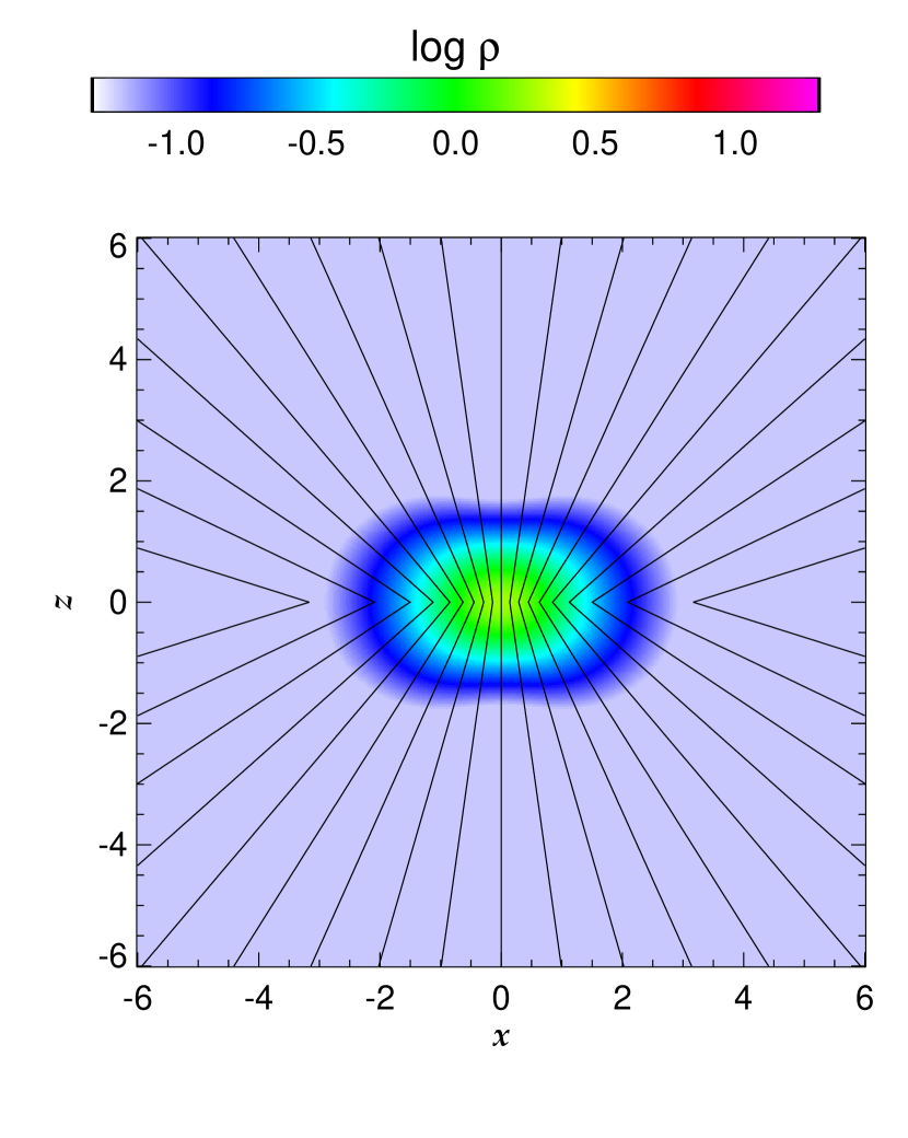
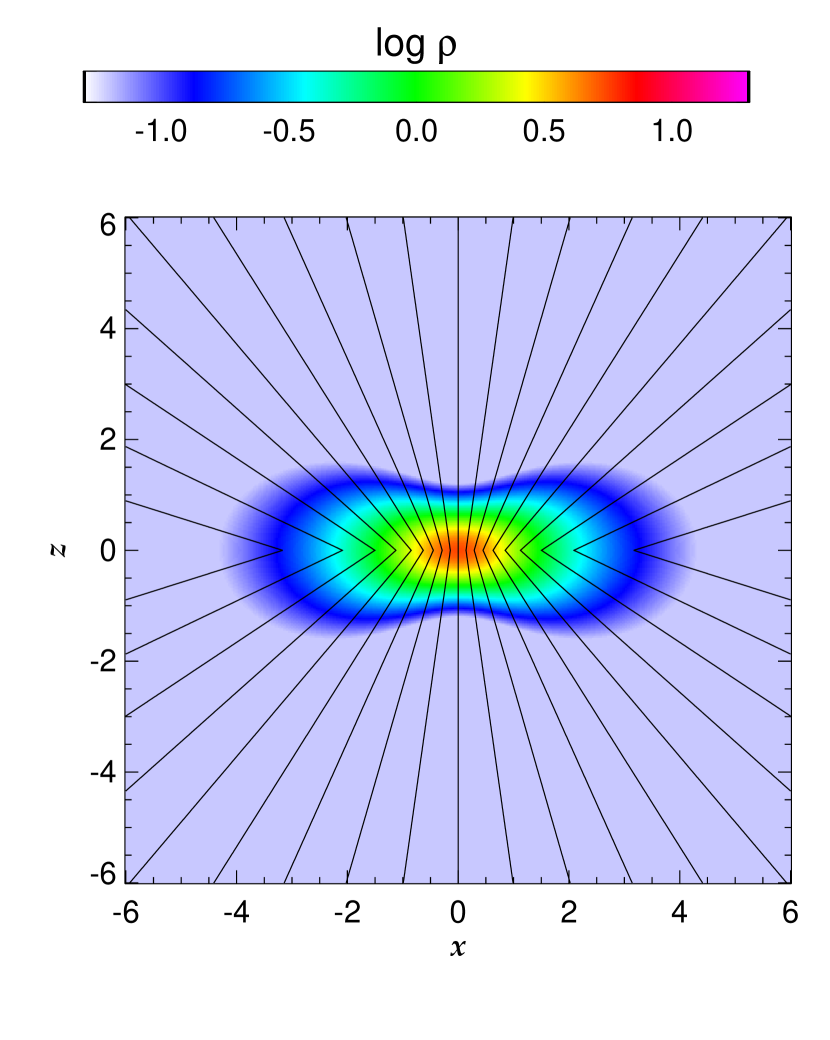
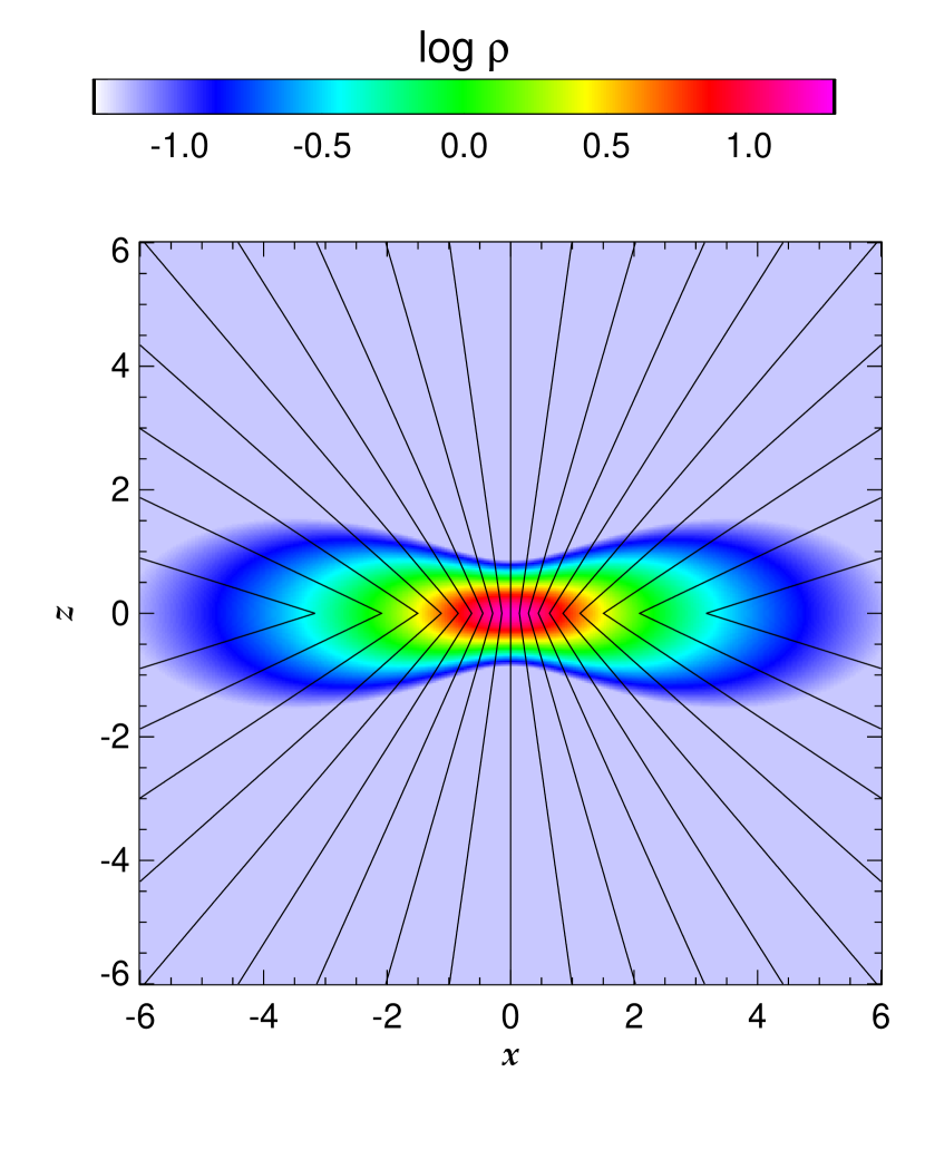
Figure 1: The cross sections show the density by color and the magnetic field by lines. The upper left and right panels are for $\lambda=5$ and $10c_{s}^{2}/G$, respectively. The bottom one is for $\lambda=20c_{s}^{2}/G$.

3 Periodically Arranged Filamentary Clouds

In this section we relax the uniform mass to flux ratio, $\Sigma/B=\mbox{const.}$, assumed in the previous section. The mass to flux ratio should increase at the cloud center through the ambipolar diffusion if the cloud is supported in part by the magnetic field against gravity. On the contrary, the mass to flux ratio decreases outside the cloud. In order to take account of magnetic field outside clouds, we consider the situation in which filamentary clouds are arranged periodically on a plane. Again each filamentary cloud is assumed to be geometrically thin. Then the surface density is given by the Fourier series,

$$\Sigma(x) = \frac{1}{\ell}\sum_{n=0}^{\infty}a_{n}\cos\left(\frac{2\pi nx}{\ell}\right),$$ (39)

where $\ell$ denotes the spacing between the filaments. The 0th Fourier series coefficient, $a_{0}$, denotes line density per each filament, $\lambda$. We obtain the gravitational potential,

$$\phi(x,z) = \frac{2\pi Ga_{0}}{\ell}|z|-\sum_{n=1}^{\infty}\frac{Ga_{n}}{n}\cos\left(\frac{2\pi nx}{\ell}\right)\exp\left(-\frac{2\pi n}{\ell}|z|\right)$$ (40)

by solving the Poisson equation. The gravity is expressed as

$$g_{x} = -\frac{2\pi G}{\ell}\sum_{n=1}^{\infty}a_{n}\sin\left(\frac{2\pi nx}{\ell}\right)\exp\left(-\frac{2\pi n}{\ell}|z|\right),$$ (41)

$$g_{z} = -\frac{2\pi G}{\ell}\frac{z}{|z|}\sum_{n=0}^{\infty}a_{n}\cos\left(\frac{2\pi nx}{\ell}\right)\exp\left(-\frac{2\pi n}{\ell}|z|\right).$$ (42)

Similarly the force free magnetic field is expressed as

$$B_{x} = -\frac{1}{\ell}\frac{z}{|z|}\sum_{n=1}^{\infty}b_{n}\sin\left(\frac{2\pi nx}{\ell}\right)\exp\left(-\frac{2\pi n}{\ell}|z|\right),$$ (43)

$$B_{z} = \frac{1}{\ell}\sum_{n=0}^{\infty}b_{n}\cos\left(\frac{2\pi nx}{\ell}\right)\exp\left(-\frac{2\pi n}{\ell}|z|\right).$$ (44)

The 0th Fourier series coefficient, $b_{0}$, denotes the magnetic flux permeating each filament, $\Phi$ in the model for an isolated filamentary cloud.

The condition for the force balance,

$$c_{s}^{2}\frac{\partial\Sigma}{\partial x}-\left.\frac{B_{x}B_{z}}{2\pi}\right|_{z=+\varepsilon} = g_{x}\Sigma,$$ (45)

is rewritten as

$$c_{s}^{2}na_{n}+\frac{1}{8\pi^{2}}\sum_{m=0}^{n}b_{m}b_{n-m}=\frac{G}{2}\sum_{m=0}^{n}a_{m}a_{n-m}.$$ (46)

This equation can be solved successively if once $\mbox{\boldmath$a$}\equiv(a_{1},a_{2},\dots)$ and $b_{0}$ are given. The Fourier series coefficient, $b_{n}$, is given by

$$b_{n} = \frac{8\pi G}{b_{0}}\left(\frac{G}{2}\sum_{m=0}^{n}a_{m}a_{n-m}-c_{s}^{2}na_{n}-\frac{1}{8\pi G}\sum_{m=1}^{n-1}b_{m}b_{n-m}\right),$$ (47)

if $a_{0}$, $\dots,a_{n}$, $b_{0}$, $\dots,b_{n-1}$ are known. In other words we can solve Equation (45) if the mass distribution and the magnetic flux are given.

In the following we consider the case,

$$a_{j} = \left\{\begin{array}[]{ll}\lambda&(j=0)\\ 2\lambda\exp(-wj)&(\mbox{otherwise})\end{array}\right.,$$ (50)

where $w$ denotes the ratio of the filament width to the interval. Then Equation (46) reduces to

$$\frac{1}{8\pi^{2}}\sum_{m=0}^{n}b_{m}b_{n-m} = 2n\lambda e^{-nw}\left(G\lambda-c_{s}^{2}\right).$$ (51)

The right hand side of this equation indicates that the gravity overcomes the pressure force when $\lambda>c_{s}^{2}/G$.

After some algebra we find a solution,

$$b_{j} = \left\{\begin{array}[]{ll}\Phi&(j=0)\\ 2\Phi\exp(-wj)&(\mbox{otherwise})\end{array}\right.,$$ (54)

$$\frac{\Phi^{2}}{4\pi^{2}} = G\lambda^{2}-c_{s}^{2}\lambda.$$ (55)

The mass to flux ratio is constant in this solution. The surface density and magnetic fields are expressed as

$$\Sigma(x,z=0) = \frac{\lambda\sinh w}{\ell\left[\cosh w-\cos\left(\displaystyle\frac{2\pi x}{\ell}\right)\right]},$$ (56)

$$B_{x}(x,z=+\varepsilon) = \frac{\Phi\sin\left(\displaystyle\frac{2\pi x}{\ell}\right)}{\ell\left[\cosh w-\cos\left(\displaystyle\frac{2\pi x}{\ell}\right)\right]},$$ (57)

$$B_{z}(x,z=0) = \frac{\Phi\sinh w}{\ell\left[\cosh w-\cos\left(\displaystyle\frac{2\pi x}{\ell}\right)\right]},$$ (58)

respectively. See Appendix A for more details on the derivation. This solution of $w=2\pi a/\ell$ approaches to that given in §2 for a given $a$ in the limit of $\ell\rightarrow\infty$ and hence $w\rightarrow 0$.

The solution obtained in the previous paragraph is a critical one. When $b_{0}$ is larger than the critical value,

$$b_{0}>2\pi\sqrt{G}\sqrt{a_{0}\left(a_{0}-\displaystyle\frac{c_{s}^{2}}{G}\right)}.$$ (59)

we obtain solutions in which the mass to flux ratio is not uniform. Equation (59) can be rewritten as

$$a_{0}<\frac{c_{s}^{2}}{2G}+\sqrt{\left(\frac{b_{0}}{2\pi\sqrt{G}}\right)^{2}+\left(\frac{c_{s}^{2}}{2G}\right)^{2}},$$ (60)

the right hand side of which denotes the maximum line density supported by magnetic flux, $b_{0}$. The filamentary clouds are confined by the magnetic pressure of the neighboring clouds. Remember that the filamentary cloud is confined by uniform magnetic field in the 2D model of Paper I. Thus the model shown in this section is closer to the 2D model than that in the previous section.

Figure 2 shows the magnetic field for $\lambda=5c_{s}^{2}/G$ and $b_{0}=10\pi c_{s}^{2}/\sqrt{G}$. The color denotes the density evaluated to be

$$\rho(x,z) \equiv \frac{\pi G\Sigma(x)^{2}}{2c_{s}^{2}}\left\{\cosh\left[\frac{\pi G\Sigma(x)z}{c_{s}^{2}}\right]\right\}^{-2},$$ (61)

in the logarithmic scale. Equation (61) denotes the equilibrium density distribution for an isothermal plane parallel disk having the surface density, $\Sigma(x)$. The magnetic field is vertical to the disk plane near $|x|=\ell/2$.

Figure 2: The cross section shows the logarithm of the density by color and the magnetic field by lines for $\lambda=5c_{s}^{2}/G$ and $\Phi=10\pi c_{s}^{2}/\sqrt{G}$. respectively.

Figure 3 shows the distribution of $B_{z}$ for models having various magnetic fluxes, $\Phi=b_{0}=9$, 10, 12, 14, 16, 18, and 20 $\pi c_{s}^{2}/\sqrt{G}$. All the models have the same line density ($\lambda=5c_{s}^{2}/G$) and accordingly the same surface density distribution shown by the dashed curve. The value of $w$ is fixed at $w=0.1$. The magnetic field and the surface density profiles are very similar near the filament axis ($x\simeq 0$). In other words almost the same amount of magnetic flux is confined in the filament and the mass to flux ratio is constant, $B_{z}=2\pi\sqrt{G}\Sigma$. When the magnetic flux is larger, the magnetic field is stronger outside the filamentary cloud. When the magnetic flux is less than a critical value ($b_{0}<9\pi c_{s}^{2}/\sqrt{G}$ in case of $\lambda=5c_{s}^{2}/G$, see Eq. (59)), we cannot construct an equilibrium model. When it is close to the critical value, the mass to flux ratio is nearly constant also outside the cloud as in the model shown in §2.

Figure 3: The solid curves denote the distribution of $B_{z}$ for $\lambda=5c_{s}^{2}/G$. The surface density is denoted by the dashed curve.

Next we compare the models having the same $\lambda$ and $\Phi$ but different $w$. Decrease in $w$ mimics quasi-static contraction since the surface density at the cloud center increases. Figure 4 denotes the mass to flux ratio at the cloud center, $2\pi\sqrt{G}\Sigma_{c}/B_{z,c}$, as a function of $\Sigma_{c}$, where $\Sigma_{c}$ and $B_{z,c}$ denote the surface density and magnetic field at $x=0$, respectively. The ordinate is denoted in unit of $c_{s}^{2}/(G\ell)$. The red curve denotes the models having $\lambda=6c_{s}^{2}/G$ and $\Phi=40\pi c_{s}^{2}/\sqrt{G}$ while the black one does those $\lambda=4c_{s}^{2}/G$ and $\Phi=40\pi c_{s}^{2}/\sqrt{G}$. As the surface density at the cloud center increases, the mass to flux ratio there increases monotonically and is saturated at

$$\left.\frac{2\pi\sqrt{G}\Sigma}{B_{z}}\right|_{\Sigma\rightarrow\infty} = \left(1-\frac{c_{s}^{2}}{G\lambda}\right)^{-1/2}.$$ (62)

Note that the mass to flux ratio tends to $\lambda/\Phi$ in the limit of $w\rightarrow\infty$ since both the surface density and magnetic field are uniform in the limit. Interestingly, however, the mass to flux ratio at the cloud center depends little on $\lambda$ for an intermediate $w$.

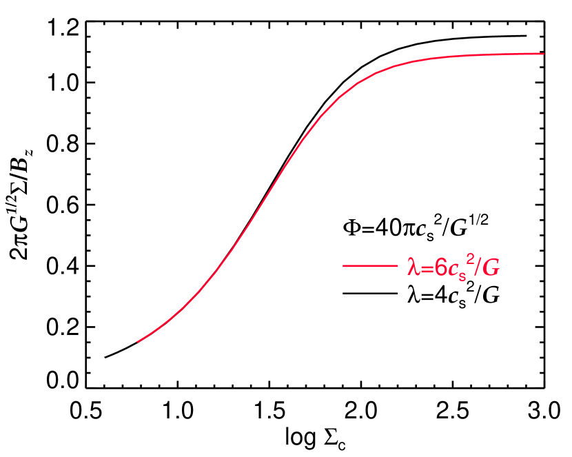
Figure 4: The mass to flux ratio at the cloud center is shown as a function of the surface density at the cloud center for given $\lambda$ and $\Phi$, which are taken to be $\lambda=4c_{s}^{2}/G$ and $\Phi=8\pi c_{s}^{2}/\sqrt{G}$ for the black curve and $\lambda=6c_{s}^{2}/G$ and $\Phi=8\pi c_{s}^{2}/\sqrt{G}$ for the red curve, respectively.

When the line density is smaller than the critical value, $c_{s}^{2}/G$, the filamentary cloud is confined not by the self-gravity but by the magnetic field. This is because the gas pressure dominates over the gravity. We can construct such a model by assuming a small $\lambda$ and a large magnetic flux. They are similar to models with small $R_{0}$ in paper I.

4 Comparison with 2D model

The thin disk model shown in §2 and 3 reproduces main features of the 2D model shown in Paper I.

Equation (27) is essentially the same as Equation (45) of Paper I,

$$2\pi R^{2}p_{s}=2c_{s}^{2}\lambda-G\lambda^{2}+\frac{\Phi_{\rm cl}^{2}}{8\pi},$$ (63)

where $R$ and $p_{s}$ denote the radius of the filament and the gas pressure at cloud surface, respectively. The symbol, $\Phi_{\rm cl}$, denotes a half of the magnetic flux permeating the filament per unit length. Equation (63) was derived from the virial analysis and the left hand side denotes the pressure force acting on the cloud surface, which vanishes in our 1D model. Differences in the numerical factors come from the assumptions used. In this paper we neglected the finite thickness of the cloud and hence pressure force acting in the $z$-direction for simplicity. Thus the critical line density is evaluated to be $\lambda_{cr}=c_{s}^{2}/G$ in case of no magnetic field ($\Phi=0$) in this paper while it should be $2c_{s}^{2}/G$ in paper I. Another difference comes from the assumed mass to flux ratio; it is uniform in the model shown in §2 while it is not in Paper I.

The following equation,

$$\lambda = \frac{c_{s}^{2}+\left(c_{s}^{4}+G\Phi_{\rm cl}^{2}/8\right)^{1/2}}{G},$$ (64)

was derived from Equation (45) of Paper I as well as Equation (28) is derived from Equation (27). Equation (64) has an asymptotic form,

$$\lambda = \frac{c_{s}^{2}}{G}+\frac{\Phi_{\rm cl}}{2\sqrt{2G}}+{\cal O}\left(\Phi_{\rm cl}^{-1}\right),$$ (65)

which resembles Equation (38) of Paper I,

$$\lambda_{\max}\simeq 0.24\frac{\Phi_{\rm cl}}{\sqrt{G}}+1.66\frac{c_{s}^{2}}{G}.$$ (66)

Equation (66) is useful since it provides an upper limit on the line density supported against gravity by magnetic field and gas pressure. The upper limit increases in proportion to the magnetic flux contained in the cloud. Thus we examine the coefficient quantitatively.

In paper I the mass to flux ratio is assumed to be the same as that of the filament having uniform density, $\rho_{0}$, and threaded by uniform magnetic field, $B_{0}$. Then the line density and magnetic flux are denoted by

$$\lambda = \pi\rho_{0}R_{0}^{2},$$ (67)

$$\Phi_{\rm cloud} = 2B_{0}R_{0},$$ (68)

respectively, where $R_{0}$ denotes the radius of the uniform filament. Note that the magnetic field surrounding but not permeating the filament is not in the count of $\Phi_{\rm cloud}$. It should be also noted that $\Phi_{\rm cloud}$ is twice as large as $\Phi_{\rm cl}$ used in Paper I. Hence, the differential mass to flux ratio is expressed as

$$\frac{d\lambda}{d\Phi} = \frac{2\lambda}{\pi\Phi_{\rm cloud}}\left[1-\left(\frac{2\Phi^{\prime}}{\Phi_{\rm cloud}}\right)\right]^{1/2},$$ (69)

$$\Phi^{\prime} \equiv \int_{0}^{x}B_{z}(x^{\prime})dx^{\prime}.$$ (70)

Here the symbols, $B_{z}(x)$ and $d\lambda/d\Phi$, denote the magnetic field on the plane of $z=0$ and mass per unit magnetic flux, respectively.

In order to evaluate the effect of the mass to flux ratio distribution, we modified the cross section of the initial filament to be

$$\left(\frac{x}{R_{0}}\right)^{2}+\left(\frac{y}{R_{0}}\right)^{2/{\cal N}} = 1,$$ (71)

where ${\cal N}\geq 0$. The initial magnetic field is again uniform at $B_{0}$. Then the mass to flux ratio is expressed as

$$\frac{d\lambda}{d\Phi} = \frac{\Gamma({\cal N}/2+3/2)}{\sqrt{\pi}\Gamma({\cal N}/2+1)}\frac{\lambda}{\Phi_{\rm cloud}}\left[1-\left(\frac{2\Phi^{\prime}}{\Phi_{\rm cloud}}\right)\right]^{{\cal N}/2},$$ (72)

where $\Gamma$ denotes the gamma function. The mass to flux ratio is uniform in the cloud when ${\cal N}=0$. On the other hand, most of the gas is filled in the magnetic field running at the center in case ${\cal N}=\infty$. Thus the parameter, ${\cal N}$, specifies the mass to flux ratio distribution as well as $w$ in the model shown in §3. See Table 1 for the ratio of the mass to flux ratio at the center to the average.

Table 1: The ratio of the central mass to flux ratio to the average.

${\cal N}$	$(d\lambda/d\Phi)_{c}/(\lambda/\Phi_{\rm cloud})$
0.0	1.0000
0.1	1.0303
0.2	1.0598
1.0	1.2732
2.0	1.5000
4.0	1.8750
10.0	2.4610

Figure 5 shows the mass to flux ratio at the cloud center, $2\pi\sqrt{G}d\lambda/d\Phi$ as a function of the density at the cloud center. Each curve denotes the locus of models having the same $\lambda$ and $\beta_{0}$, where $\beta_{0}\equiv\rho_{s}c_{s}^{2}(B_{0}^{2}/8\pi)^{-1}$ denotes the initial plasma beta in the ambient gas surrounding the filamentary cloud. As in Paper I, the model clouds are assumed to be confined by a very tenuous gas of which pressure is $\rho_{s}c_{s}^{2}$. The density at the cloud center is measured in unit of $B_{0}^{2}/(8\pi c_{s}^{2})$. Thus the abscissa denotes the ratio of the gas pressure at the cloud center to the magnetic pressure in the region very far from the cloud, since the magnetic field is nearly uniform at the initial value, $B_{0}$, in our 2D model. The line density is specified in unit of $c_{s}^{2}/G$ on the diagram.

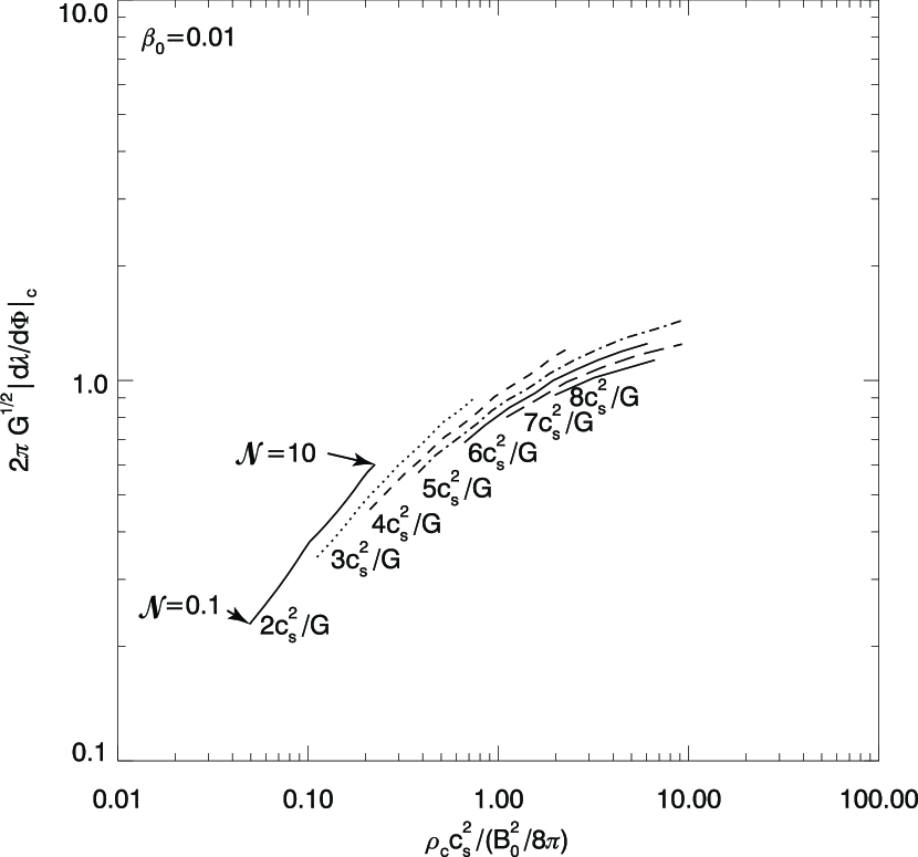
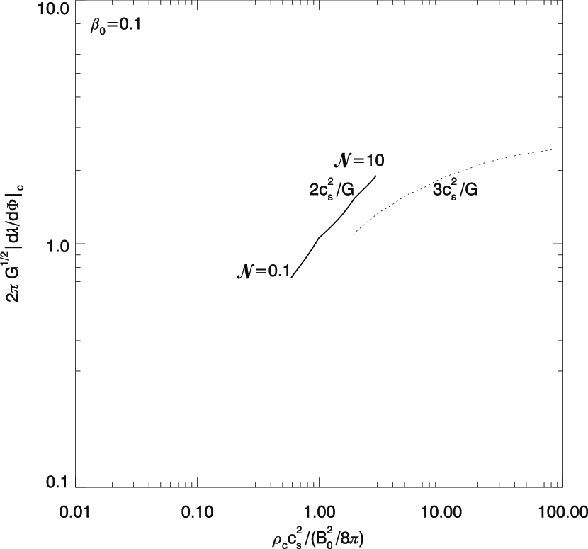
Figure 5: The mass to flux ratio at the cloud center is shown as a function of the density thereof in 2D models. The curves denote the loci of constant $\lambda$ of which values are labelled. The central density is denoted in unit of $B_{0}^{2}/8\pi c_{s}^{2}$. The index, ${\cal N}$, increases from left to right along the loci. The left and right panels denote the models of $\beta_{0}=0.01$ and 0.1, respectively.

The index, ${\cal N}$, increases from ${\cal N}=0.1$ (left) to 10 (right) on each locus. This means that the filamentary cloud is more centrally condensed and the central mass to flux ratio is higher when ${\cal N}$ is larger. The mass to flux ratio depends only a little on $\lambda$ in the models of $\beta_{0}=0.01$. This is because the gas is relatively cold and accordingly the gas pressure has only minor contribution to the cloud support. Note that the mass to flux ratio is slightly larger for a smaller $\lambda$ when $\rho_{c}$ is given. The maximum non-dimensional mass to flux ratio is only slightly larger than unity when $\lambda\geq 5c_{s}^{2}/G$ and $\beta_{0}=0.01$.

When $\beta_{0}=0.1$, the gas is relatively warm and hence the pressure has a significant contribution to the cloud support. The non-dimensional mass to flux ratio is significantly higher than unity especially when $\rho_{c}>B_{0}^{2}/(8\pi c_{s}^{2})$, although it is still less than three. This high mass to flux ratio is realized only when the cloud is relatively warm and the line density is relatively small.

The maximum line density depends also on ${\cal N}$, i.e., $\lambda_{\max}=\lambda_{\max}(\Phi_{\rm cl},c_{s},{\cal N})$. Equation (46) of Paper is that for ${\cal N}=1$. When $\Phi_{\rm cl}$ and $c_{s}$ are given, the maximum line density is lower for a larger ${\cal N}$. Increase in ${\cal N}$ mimics the quasi-static evolution of a molecular cloud by the ambipolar diffusion. As ${\cal N}$ approaches to zero, the maximum line density tends to the value given by Equation (28).

5 Stability Against Fragmentation

We consider the stability of the isolated filamentary cloud against fragmentation, i.e., a sinusoidal perturbation in the $z$-direction. The gas is assumed to be still confined in the plane of $z=0$ and we use the method of images to obtain the changes in the gravity and density consistently. The image density is assumed to have the form,

$$\varrho(x,y,z) = \varrho_{0}(x,z)+\varrho_{1}(x,y,z),$$ (73)

$$\varrho_{0}(x,z) = 2\lambda\delta(x)\delta(z+a),$$ (74)

$$\varrho_{1}(x,y,z) = \int_{0}^{\infty}\delta\lambda(b)\cos ky\delta(x)\delta(z+b)db,$$ (75)

for calculating the change in the gravity in the upper half space of $z>0$. The change in the gravity is evaluated as

$$\delta g_{z}(x,y,z=+\varepsilon) = -G\int_{-\infty}^{+\infty}\frac{(z-z^{\prime})\varrho_{1}(x^{\prime},y^{\prime},z^{\prime})}{\left[(x-x^{\prime})^{2}+(y-y^{\prime})^{2}+(z^{\prime})^{2}\right]^{3/2}}dx^{\prime}dy^{\prime}dz^{\prime}$$ (76)

$$= -Gb\cos ky\int_{-\infty}^{+\infty}\int_{0}^{\infty}\frac{\delta\lambda(b)\cos ks}{\left(x^{2}+s^{2}+b^{2}\right)^{3/2}}dsdb$$ (77)

$$= -2Gkb\cos ky\int_{0}^{\infty}\frac{\delta\lambda(b)K_{1}\left(k\sqrt{x^{2}+b^{2}}\right)}{\sqrt{x^{2}+b^{2}}}db,$$ (78)

where $K_{1}$ denotes the modified Bessel function of the 1st order. Here we used the mathematical formula (Abramowicz & Stegun, 1965),

$$K_{\nu}(z) = \Gamma\left(\nu+\displaystyle\frac{1}{2}\right)\frac{\left(2z\right)^{\nu}}{\sqrt{\pi}}\int_{0}^{\infty}\frac{\cos t}{\left(t^{2}+z^{2}\right)^{\nu+1/2}}dt.$$ (79)

Similarly we obtain

$$\delta g_{x} = -2Gk\cos ky\int_{0}^{\infty}\frac{x\delta\lambda(b)K_{1}\left(k\sqrt{x^{2}+b^{2}}\right)}{\sqrt{x^{2}+b^{2}}}db,$$ (80)

$$\delta g_{y} = 2Gk\sin ky\int_{0}^{\infty}\delta\lambda(b)K_{0}\left(k\sqrt{x^{2}+b^{2}}\right)db.$$ (81)

The change in the surface density is expressed as

$$\delta\Sigma(x,y,z=0) = \frac{kb\cos ky}{\pi}\int_{0}^{\infty}\frac{\delta\lambda(b)K_{1}\left(k\sqrt{x^{2}+b^{2}}\right)}{\sqrt{x^{2}+b^{2}}}db.$$ (82)

The magnetic field is assumed to be aligned with the gravity also in the perturbed state. This assumption is reasonable since the gas density is quite low and hence the inertia is negligibly small outside the cloud ($z\neq 0$). The magnetic field is still current free and does not extract any momentum from the cloud. Then the change in the magnetic field are expressed as

$$\delta B_{x} = -\frac{\alpha}{\sqrt{G}}\delta g_{x},$$ (83)

$$\delta B_{y} = -\frac{\alpha}{\sqrt{G}}\delta g_{y},$$ (84)

$$\delta B_{z} = -\frac{\alpha}{\sqrt{G}}\delta g_{z},$$ (85)

in $z>0$. Both the gravity and magnetic field change with the time in proportion to $\exp(-i\omega t)$, where $\omega$ denotes the angular frequency of the perturbation.

We use the displacement vector,

$$\xi = \left(\begin{array}[]{c}\xi_{x}\cos ky\\ \xi_{y}\sin ky\end{array}\right)\exp(-i\omega t),$$ (88)

for our stability analysis. The $y$-dependence of the displacement vector is chosen so that the the equation of mass conservation be the ordinary differential equation with respect to $x$,

$$\delta\Sigma+\frac{d}{dx}\left(\xi_{x}\Sigma_{0}\right)+k\xi_{y}\Sigma_{0} = 0,$$ (89)

where $\Sigma_{0}$ denotes the surface density in the equilibrium. Also the equation of motion reduces to the ordinary differential equation and algebraic equation,

$$-\omega^{2}\Sigma_{0}\xi_{x}+c_{s}^{2}\frac{d}{dx}\delta\Sigma-\left(1-\alpha^{2}\right)\left(\Sigma_{0}\delta g_{x}+g_{x}\delta\Sigma\right) = 0,$$ (90)

$$-\omega^{2}\Sigma_{0}\xi_{y}-c_{s}^{2}k\delta\Sigma+\left(1-\alpha^{2}\right)\Sigma_{0}\delta g_{y} = 0.$$ (91)

It is difficult to solve Equations (89) through (91) simultaneously since they are associated with Equation (78), (80) and (81). Instead of solving the equations we use the variational principle to evaluate $\omega^{2}$. First we rewrite Equations (90) and (91) into

$$-\omega^{2}\xi_{x}+c_{s}^{2}\frac{d}{dx}\left(\frac{\delta\Sigma}{\Sigma_{0}}\right)-\left(1-\alpha^{2}\right)\delta g_{x} = 0,$$ (92)

$$-\omega^{2}\xi_{y}+c_{s}^{2}k\frac{\delta\Sigma}{\Sigma_{0}}+(1-\alpha^{2})\delta g_{y} = 0,$$ (93)

by using the condition for magnetohydrostatic equilibrium,

$$c_{s}^{2}\frac{d}{dx}\Sigma_{0}-\left(1-\alpha^{2}\right)\Sigma_{0}g_{x} = 0.$$ (94)

Note that the displacement is irrotational,

$$\frac{d\xi_{y}}{dx}+k\xi_{x} = 0,$$ (95)

since angular momentum extraction by magnetic field is not taken into account. We obtain

$$-\omega^{2}\Sigma_{0}\left(\xi_{x}^{2}+\xi_{y}^{2}\right)+c_{s}^{2}\frac{\delta\Sigma^{2}}{\Sigma_{0}}-\left(1-\alpha^{2}\right)\Sigma_{0}\left(\xi_{x}\delta g_{x}+\xi_{y}\delta g_{y}\right)+\frac{d}{dx}\left(c_{s}^{2}\xi_{x}\delta\Sigma\right) = 0,$$ (96)

by taking the sum of the products of $c_{s}^{2}\delta\Sigma/\Sigma_{0}$ and Equation (89), $\xi_{x}\Sigma_{0}$ and Equation (92), $\xi_{y}\Sigma_{0}$ and Equation (93). We obtain

$$\omega^{2} = \frac{\displaystyle\int_{-\infty}^{+\infty}\Sigma_{0}\left[c_{s}^{2}\left(\frac{\delta\Sigma}{\Sigma_{0}}\right)^{2}-\left(1-\alpha^{2}\right)\left(\xi_{x}\delta g_{x}+\xi_{y}\delta g_{y}\right)\right]dx}{\displaystyle\int_{-\infty}^{+\infty}\Sigma_{0}\left(\xi_{x}^{2}\,+\,\xi_{y}^{2}\right)dx}$$ (97)

$$= c_{s}^{2}\frac{\displaystyle\int_{-\infty}^{+\infty}\Sigma_{0}\left[\left(\frac{\delta\Sigma}{\Sigma_{0}}\right)^{2}-\frac{1}{G\lambda}\left(\xi_{x}\delta g_{x}+\xi_{y}\delta g_{y}\right)\right]dx}{\displaystyle\int_{-\infty}^{+\infty}\Sigma_{0}\left(\xi_{x}^{2}\,+\,\xi_{y}^{2}\right)dx}$$ (98)

by integrating Equation (96) and submitting $\xi_{x}=0$ at $x=\pm\infty$. The right hand side of Equation (98) gives a lower bound for the eigenvalue, $\omega^{2}$, when an arbitrary perturbation is substituted. If it is negative for a given perturbation, the filament is unstable.

We evaluate the right hand side of Equation (98) as a functional of the change in the image density, $\delta\lambda(b)$. The change in the gravity is evaluated by numerical integral of (80), and (81). The change in the surface density is evaluated by the numerical integral of (82). The displacement, $\xi_{x}$, is obtained by solving the ordinary differential equation,

$$\frac{d}{dx}\left(\frac{\delta\Sigma}{\Sigma_{0}}\right)+\frac{d}{dx}\left[\frac{1}{\Sigma_{0}}\frac{d}{dx}\left(\Sigma_{0}\xi_{x}\right)\right]-k^{2}\Sigma_{0}\xi_{x} = 0,$$ (99)

which is obtained by combining Equations (89) and (95). The displacement, $\xi_{y}$ is obtained simultaneously when we solve Equation (99). The above mentioned procedure allows us to evaluate the right hand side of Equation (98) as a functional of $\delta\lambda$. See Appendix B for more details.

As shown in the previous section, FWHM of our model cloud (=$a$) is not specified by the condition for magnetohydrostatic equilibrium. If the filamentary cloud has proper line density and magnetic flux, it can be settled in equilibrium at any width. This means that our model cloud is neutrally stable for perturbation having $k=0$. As in the case of longitudinal or helical magnetic field, we use the non-dimensional wavenumber, $ka$, in our analysis.

In this paper we consider two types of trial functions for the variational principle. Type I trial function is expressed as

$$\delta\lambda_{1}(b) = \delta\left(b-\beta a\right),$$ (100)

where $\beta$ is chosen to minimize the value of $-\omega^{2}$. Type II is expressed as

$$\delta\lambda_{2}(b) = \sum_{j=1}^{N}\theta_{j}\delta\left(b-\beta_{j}a\right),$$ (101)

where a set of $\theta_{j}$ is chosen to minimize the value of $\omega^{2}$ for fixed $\beta_{j}$.

The left panel of Figure 6 shows the growth rate obtained by applying type I trial function. The abscissa is the wavenumber in unit of $a^{-1}$ while the ordinate is the growth rate in unit of $(c_{s}/a)^{2}$. The right panel of Figure 6 shows that obtained by applying type II trial function in which the values of $\beta_{i}$ are taken to be $\mbox{\boldmath$\beta$}=(1.0,1.4,1.8,2.2,2.6)$. Our model filamentary clouds are unstable against fragmentation as well as the filamentary clouds threaded by longitudinal magnetic field. The most unstable mode has the wave number, $k_{\max}\simeq 0.8a^{-1}$, and the growth rate, $|\omega|\simeq 0.6c_{s}a^{-1}$, irrespectively of $\lambda$.

Figure 6: The growth rate is shown as a function of the longitudinal wavenumber. It is derived by applying the type I and type II trial functions to the variational principle, in left and right panels, respectively. See text for further details.

6 Discussions and Summary

As shown in the previous sections, our 1D model based on the thin disk approximation reproduces the main features of 2D model shown in paper I. The maximum mass sustained by magnetic field is roughly proportional to the magnetic flux. The critical mass to flux ratio depends on the mass loading, i.e., the distribution of $\Sigma/B$. When the mass loading is uniform ($\Sigma/B=$ const.), it is slightly larger than $\lambda/B_{z}>(2\pi\sqrt{G})^{-1}$. The same critical ratio is obtained for disks in equilibrium and slabs stable against fragmentation. Remember that Strittmatter (1966) obtained a similar value from the viral analysis on the magnetohydrostatic equilibrium. The critical ratio seems to depend little on the cloud geometry. Remember that filamentary clouds with a longitudinal field are unstable against fragmentation even if the magnetic field is very strong. The instability is due to the fact that the mass to flux ratio is infinitely large since the clouds are highly extended in the direction of magnetic field.

Given the critical mass to flux ratio depends little on the cloud geometry, then it can be applied to the stability of periodically arranged filamentary clouds. They are almost isolated each other in the limit of $w\rightarrow 0$. Thus they are unstable against fragmentation as well as the isolated filamentary clouds since the mass to flux ratio is larger than the critical value at the cloud center ($\Sigma_{c}>2\pi\sqrt{G}B_{z,c}$). When $w\rightarrow\infty$, our 1D model reduces to a slab of which stability was already investigated by Nakano & Nakamura (1978). The slab is stable as far as $\Sigma<2\pi\sqrt{G}B$. In short the models shown in Figure 4 are stable/unstable for small/large value of $\Sigma_{c}$. We surmise that the models of $\Sigma_{c}<2\pi\sqrt{G}B_{z,c}$ are stable against fragmentation. Most of the 2D models shown in Figure 5 are also likely to be stable against fragmentation since $\Sigma_{c}<2\pi\sqrt{G}B_{z,c}$.

The above argument brings us an interesting result. Filamentary clouds supported by longitudinal magnetic fields are unstable against fragmentation while those supported by perpendicular fields can be stable. The latter can collapse quasi-statically through ambipolar diffusion, while the former cannot.

Our models are still idealistic since turbulence and other dynamical effects are not taken into account. Nevertheless, they provide physical insights on the dynamics of filamentary clouds. Filamentary clouds with perpendicular magnetic field are likely to be able to sustain their forms as far as they are subcritical at the cloud center. They may fragment after the mass to flux ratio exceeds the critical value by ambipolar diffusion or by mass accretion along the magnetic field (Heitsch & Hartmann, 2014).

This work was supported in part by JSPS KAKENHI Grant Number 24540226.

Appendix A Fourier Series

We used the mathematical formula,

$$\sum_{n=0}^{\infty}a^{n}\cos nx = \frac{a\cos x-a^{2}}{1-2a\cos x+a^{2}},$$ (A1)

for $|a|<1$ in order to derive Equation (56) from Equations (39) and (50). The gravitational potential, $\phi$, and the $y$-component of the vector potential, $A_{y}$, are expressed as

$$\phi = \frac{2\pi G\lambda}{\ell}|z|-\sum_{n=1}^{\infty}\frac{G\lambda}{n}\cos\left(\frac{2\pi nx}{\ell}\right)\exp\left[-n\left(w+\frac{2\pi}{\ell}|z|\right)\right],$$ (A2)

$$A_{y} = \frac{\Phi x}{\ell}+\sum_{n=1}^{\infty}\frac{\Phi}{\pi n}\sin\frac{2\pi nx}{\ell}\exp\left[-n\left(w+\frac{2\pi}{\ell}|z|\right)\right],$$ (A3)

respectively, for the solution specified by Equations (56) through (58). They are also expressed as

$$\phi = -G\lambda\log\left[\cosh\left(w+\frac{2\pi|z|}{\ell}\right)-\cos\left(\frac{2\pi x}{\ell}\right)\right],$$ (A4)

$$A_{y} = \frac{\Phi}{\pi}\tan^{-1}\left[\frac{\tan\left(\displaystyle\frac{\pi x}{\ell}\right)}{\tanh\left(\displaystyle\frac{w}{2}+\displaystyle\frac{\pi|z|}{\ell}\right)}\right],$$ (A5)

respectively, since

$$\sum_{n=1}^{\infty}\frac{a^{n}}{n}\cos nx = -\frac{1}{2}\log\left(1-2a\cos x+a^{2}\right),$$ (A6)

$$\sum_{n=1}^{\infty}\frac{a^{n}}{n}\sin nx = \tan^{-1}\left(\frac{a\sin x}{1-a\cos x}\right),$$ (A7)

for $|a|\leq 1$.

Appendix B Perturbation Equations

For a given $\delta\Sigma$ we obtain $\xi_{x}$ and $\xi_{y}$ by the following procedure.

First we rewrite Equations (99) and (95) as

$$\frac{d\xi_{x}}{dx} = -\frac{d\ln\Sigma_{0}}{dx}\xi_{x}-k\xi_{y}-\frac{\delta\Sigma}{\Sigma_{0}},$$ (B1)

$$\frac{d\xi_{y}}{dx} = -k\xi_{x}.$$ (B2)

We consider the case in which $\delta\Sigma$ and $\xi_{x}$ are symmetric and antisymmetric with respect to $x$, respectively. This choice is rational since the unperturbed state is symmetric and we are interested in the gravitational instability. An eigenmode perturbation should be either symmetric or antisymmetric and the fragmentation of a filamentary cloud is symmetric with respect to $x$. Thus we obtain the boundary condition, $\xi_{x}=0$ at $x=0$. We assume that the displacement diminishes in the form,

$$\xi_{x}\propto\exp\left(-kx\right),$$ (B3)

$$\xi_{y}\propto\exp\left(-kx\right),$$ (B4)

in the limit of $x\rightarrow+\infty$. This choice is based on the fact that the relative change in the surface density is proportional to $\exp(-kx)$ in the limit. Equations (B3) and (B4) are valid also when $\delta\Sigma/\Sigma_{0}$ decreases more steeply with increase in $x$.

We integrate Equations (B1) and (B2) from $x=0$ to $x_{\rm out}$ with stepsize $\Delta x=5\times 10^{-2}$ by the 4th order Runge-Kutta method to obtain two sets of solutions. One has initial condition $(\xi_{x},d\xi_{x}/dx)=(0,0)$. The other is the solution of Equations (B1) and (B2) without the source term, i.e., the homogenous one and has the initial condition $(\xi_{x},d\xi_{x}/dx)=(0,1)$. We obtain the solution satisfying the boundary conditions at $x=0$ and $x_{\rm out}$ as a linear combination of them. The outer boundary is set at $x_{\rm out}=\min(15k^{-1},40)$. The $y$-component of the displacement, $\xi_{y}$, is derived from Equation (95).

Now we can evaluate the right hand side of Equation (98) for a given $\delta\lambda(b)$. Consequently the growth rate is evaluated to be a function of $b$ in type I trial function. We searched for $b$ which maximizes the growth rate in the interval of $0.55a\leq b\leq 2.5a$ with the interval $\Delta b=0.05a$. Both the denominator and delimiter of the right hand side of Equation (98) are the quadratic expressions of $\theta_{1},\dots,\theta_{5}$, when type II trial function is used. We used LAPACK, a mathematical library for linear algebra installed in IDL, the interactive data language, for minimizing $-\omega^{2}$.

We used the public Fortran subroutines downloaded from Prof. Jian-ming Jin’s web page (jin.ece.illinois.edu) to obtain the numerical values of the modified Bessel functions.

References

- Abramowicz & Stegun (1965) Abramowicz, M., Stegun, I.A. 1965, Handbook of Mathematical Functions with Formulas, Graphs and Mathematical Tables, New York, Dover
- Binney & Tremaine (2008) Binney, J., Tremaine, S. 2008, Galactic Dynamics, 2nd ed. Princeton, Princeton Univ. Press, Sec. 2.6
- Goodman et al (1990) Goodman, A.A., Bastien, P., Myers, P.C., Ménard, F. ApJ, 359, 363
- Hanawa et al. (1993) Hanawa, T., Nakamura, F., Matsumoto, T. et al. 1993, ApJ, 404, L83
- Heitsch & Hartmann (2014) Heitsch, F. & Hartmann, L. 2014, MNRAS, 443, 230
- Mestel & Paris (1984) Mestel, L., Paris, R.B. 1984, A&A, 136, 98
- Mestel & Spitzer (1956) Mestel, L., Spitzer, Jr., L. 1956, MNRAS, 116, 503
- Moneti et al. (1984) Moneti, A., Pipher, J. L., Helfer, H. L. et al. ApJ, 282, 508
- Mouschovias (1976a) Mouschovias, T.C. 1976a, ApJ, 206, 753
- Mouschovias (1976b) Mouschovias, T.C. 1976b, ApJ, 207, 141
- Nakamura et al. (1995) Nakamura, F., Hanawa, T., Nakano, T. 1995, ApJ, 444, 700
- Nakano & Nakamura (1978) Nakano, T., Nakamura, T. 1978, PASJ, 30, 671
- Ostriker (1964) Ostriker, J. 1964, ApJ, 140, 1056
- Palmeirim et al. (2013) Palmeirim, P., André, Ph., Kirk, J., et al. A&A, 550, A38
- Pereyra & Magahães (2004) Pereyra, A., Magahães, A.M. 2004, ApJ, 603, 584
- Shu & Li (1997) Shu, F.H., Li, Z.-Y. 1997, ApJ, 475, 251
- Stodółkiewcz (1963) Stodółkiewicz, J.S. 1963, AcA, 13, 30
- Strittmatter (1966) Strittmatter, P.A. 1966, MNRAS, 132, 359
- Tomisaka (1991) Tomisaka, K. 1991, ApJ, 376, 190
- Tomisaka (1995) Tomisaka, K. 1995, ApJ, 438, 226
- Tomisaka, Ikeuchi & Nakamura (1988) Tomisaka, K., Ikeuchi, S., Nakamura, T. 1988, ApJ, 335, 239
- Tomisaka (2014) — 2014, ApJ, 785, 24