Blob indentation identification via curvature measurement

Abstract

This paper presents a novel method for identifying indentations on the boundary of solid 2D shape. It uses the signed curvature at a set of points along the boundary to identify indentations and provides one parameter for tuning the selection mechanism for discriminating indentations from other boundary irregularities. An efficient implementation is described based on the Fourier transform for calculating curvature from a sequence of points obtained from the boundary of a binary blob.

Index Terms—  blob analysis, shape indentations, curvature, Fourier transform

1 Introduction

Blob detection is a common unit in image processing pipelines in which an image is reduced to a set of distinct solid connected components that are then analyzed further. Most image processing packages provide a number of useful geometric and topological quantities that can be computed for blobs, such as their centroid, area, eccentricity, perimeter, and so on. In some applications it is important to look at properties of the boundary of the blobs. In particular, indentations and irregularities in the shape boundary that may have specific meaning in a given domain (e.g., irregularly shaped cells in microscopy, defective widgets in manufacturing, etc…). How does one go about characterizing these indentations and irregularities to count them, locate them, and measure them?

In this paper a method is presented to analyze blob boundaries to identify indentations based on deriving a parameterized curve enclosing the blob and using measures of curvature on this curve to determine where indentations are present. A trigonometric polynomial representation of the boundary curve is obtained via the Fourier transform, and the necessary derivatives to compute the signed curvature are obtained using convenient properties of the Fourier transform that make such computations very simple to state and implement. This method requires one parameter, severity, for tuning what constitutes an indentation versus a simple irregularity in the shape. This parameter has a geometric interpretation related to the radius of curvature along the boundary giving indentation selection a natural length scale. The method will be briefly compared with other approaches to this problem using common algorithms such as the convex hull of the shape to demonstrate where this method is preferable.

2 Approach

The key tool used in this method is the interpretation of the boundary of the shape as a parametric curve from which one can compute the approximate curvature at a sequence of points. When the sign of the curvature changes (i.e., when the normal to the curve switches from pointing into the shape to outside, or vice versa), one can infer that an inflection point has occurred corresponding to an indentation beginning or ending. The steps of the algorithm are:

• Derivation of a trigonometric polynomial representation of the discrete blob boundary point sequence as a continuous curve parameterized by arc length from an arbitrary boundary starting position.

• Optional low-pass filtering of the parameterized boundary curve. This step eliminates high-frequency oscillations in the curve due to the discretization of the continuous shape when pixelized.

• Calculation of the first and second derivative along the curve by element-wise multiplication in the frequency domain. Reconstruction of the first and second derivative in the spatial domain necessary to calculate the curvature along the boundary is obtained via the inverse Fourier transform.

• Identification of inflection points along the curve at points of curvature sign change. The regions delimited by these inflection points are then filtered by radius of curvature to eliminate detection of non-indentation features.

A prerequisite for this algorithm is an existing segmentation pipeline that yields binary blobs from images, as well as a method for extracting an ordered point sequence along the boundary of these blobs. Such methods exist in many off-the-shelf software packages (such as the MATLAB image processing toolbox).

2.1 Related approaches

Shape analysis is a widespread activity in image processing. The majority of techniques found in the literature or published software packages rely on working directly with the pixel boundary of a shape or a polygon approximation for either the shape or its convex hull. The use of the convex hull for providing an approximation for a shape from which other properties can be easily computed is popular in large part due to the algorithmic efficiency and widespread availability of convex hull algorithms in popular packages using the QuickHull method [1, 2]. As discussed later in Section 5.2, these methods make significant assumptions about what constitutes a shape indentation limiting their utility.

Approaches that do not make assumptions about how indentations relate to the convex hull of a shape are more robust to diverse shapes. Alpha shapes [3, 4] and Delaunay triangulations [5] can be used to calculate a boundary of an image from a point set (e.g., a set of pixels identified along the boundary of a binary blob). These methods unfortunately still require heuristic tests to determine when an indentation occurs given that the decision as to whether or not an indentation is present requires more information than can be derived from a single boundary line segment or vertex.

The calculation of the curvature using a Fourier series to represent the boundary curve naturally takes into account all points along the boundary. As such, the calculation of curvature at any point along the curve is intrinsically informed by the properties of the entire curve removing the need for any local heuristics near the point where curvature is calculated. This simplifies the algorithm by removing heuristics that would induce additional parameters and potential points of brittleness.

3 Curvature calculation

Given a blob with a corresponding boundary pixel sequence $B=((x_{1},y_{1}),...,(x_{n},y_{n}))$, the goal is to calculate the curvature $\kappa$ at each point along $B$. The signed curvature can be defined at the $i$th point along the curve in terms of the local first and second derivatives at that point:

$$\kappa_{i}=\frac{x_{i}^{\prime}y_{i}^{\prime\prime}-y_{i}^{\prime}x_{i}^{\prime\prime}}{\left({x_{i}^{\prime}}^{2}+{y_{i}^{\prime}}^{2}\right)^{\frac{3}{2}}}$$ (1)

The derivatives along $B$ must be calculated from the point sequence that was derived from the blob boundary. A simple and fast method for achieving this is via the Fourier transform [6]. The Fourier transform has a very convenient property that allows for simple calculations of derivatives of any function represented as a Fourier series. Given some function $x(t)$, the following property holds for its derivatives:

$$\mathcal{F}\left[\frac{d^{n}}{dt^{n}}x(t)\right]=(i\omega)^{n}X(i\omega)$$ (2)

Where $X(i\omega)=\mathcal{F}[x(t)]$. This allows the function to be differentiated in the frequency domain via simple multiplication. In the case of blob boundaries, the function $x(t)$ can be replaced by the sampled boundary points $x[t]$. The $n$th derivative in the spatial domain necessary for the calculation of $\kappa$ is recovered via the inverse Fourier transform:

$$x^{(n)}(t)=\mathcal{F}^{-1}\left[(i\omega)^{n}X(i\omega)\right]$$ (3)

This approach is attractive for a number of reasons. First, the Fourier representation does not use a spatially local approximation for the curve in calculating the derivatives. This eliminates the need to select parameters such as a stencil size when using finite difference approximations for calculating derivatives directly from the boundary point sequence. Second, once the boundary curve has been moved to the frequency domain additional processing is possible to address issues such as high-frequency oscillations along a boundary due to pixel-level effects. Application of low-pass filters is very simple in the frequency domain and composes cleanly with the calculation of the derivative. In fact, any additional processing of the shape boundary that can be represented via convolutions can be included in the calculations applied to the boundary while in the frequency domain.

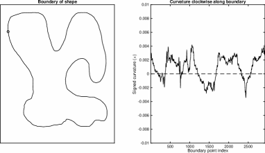
Fig. 1: Illustration of a parameterized curve boundary and the corresponding curvature measure along the boundary (clockwise, starting at indicated point on boundary.)

4 Indentation identification

Identifying indentations on a blob boundary using curvature requires searching for inflection points where the normal to the curve changes sign. This occurs at points where the curvature reaches zero. Consider the example blob in Figure 1. The curvature along the curve is shown in the right-hand plot, showing clearly the points along the curve where the curvature passes through zero.

One parameter is used to tune indentation selection, severity ($\sigma$). This parameter has a close relationship with the radius of curvature that is used to define what constitutes an indentation. The magnitude of curvature, $|\kappa|$, at a point along the boundary can be related to the radius $\rho$ of the circular arc that fits the curve at that point [7]:

$$\frac{1}{|\kappa|}\propto\rho$$ (4)

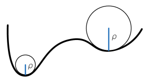
Fig. 2: An illustration for the radius of curvature for different sized indentations.

In regions of very low magnitude curvature, the corresponding circular arc would have a very large radius. Similarly, when the magnitude of curvature is high, the best-fit circular arc would have a low radius. Indentations can be thought of as places on the boundary where the sign of curvature is negative and the magnitude of curvature is high, and the use of the radius of curvature can provide a cutoff length scale for filtering indentations from non-indentation irregularities in which the sign of curvature is also negative.

Given a maximum radius of curvature for what would be considered an indentation, $\rho_{\sigma}$, then $\rho<\rho_{\sigma}$ can be interpreted with respect to curvature by Eq. 4 as $|\kappa|^{-1}<\sigma^{-1}$. Thus indentations will be considered only when $|\kappa|>\sigma$.

5 Algorithm

The algorithm for the curvature calculation can be specified in MATLAB as follows:

⬇

ction k = curvature(xs, ys)

fxs = fft(xs); fys = fft(ys);

nx = length(xs);

hx = ceil(nx/2)-1;

ftdiff = (2i*pi/nx)*(0:hx);

ftdiff(nx:-1:nx-hx+1) = -ftdiff(2:hx+1);

ftddiff = (-(2i*pi/nx)^2)*(0:hx);

ftddiff(nx:-1:nx-hx+1) = ftddiff(2:hx+1);

dx = real(ifft(fxs.*ftdiff'));

dy = real(ifft(fys.*ftdiff'));

ddx = real(ifft(fxs.*ftddiff'));

ddy = real(ifft(fys.*ftddiff'));

k = (ddy.*dx-ddx.*dy) ./ ((dx.^2+dy.^2).^(3/2));

end

First, the x and y coordinate arrays of the points along the curve are mapped to the frequency domain with the FFT. The differential operator is calculated based on the length of the point sequences based on Eq. 2. This operator is then applied by pointwise multiplication against the frequency representation of the points and the first and second spatial derivatives are then obtained by taking the real component of the inverse Fourier transform of the products (Eq. 3). The calculation of $\kappa$ then follows exactly as defined in Eq. 1.

Identification and counting of indentations then requires processing of the curvature sequence, as performed in the following pseudocode.

⬇

ction n = countindentations(k, sigma)

ksigns = sign(k);

ksignchanges = diff(ksigns);

idxchanges = [1; find(ksignchanges); ...

length(ksignchanges)];

n = 0;

for i = 1:length(idxchanges)-1

ks = k(idxchanges(i):idxchanges(i+1));

if mean(ks) < 0 && max(abs(ks)) > sigma

n = n + 1;

end

end

return n

end

This algorithm takes the curvature sequence k and identifies where sign changes occur. This is used to partition the curvature sequence into a set of regions with the same sign curvature. Each is then examined to identify those that represent negative curvature regions in which the maximum curvature exceeds the value of the severity parameter sigma.

5.1 Demonstration

The application of this algorithm is shown in Figure 3 for six different shapes: two synthetic blobs drawn by hand, and four blobs derived from photographs of different types of flowers. In each of the sub-images the regions of negative curvature are indicated by the heavy boundary curve, and the title indicates the number of indentations that were detected. In some cases the effect of the $\sigma$ parameter is apparent where irregularities along the surface were ruled out as indentations since their maximum curvature did not exceed the threshold corresponding to the acceptable range of radii of curvature for indentations.

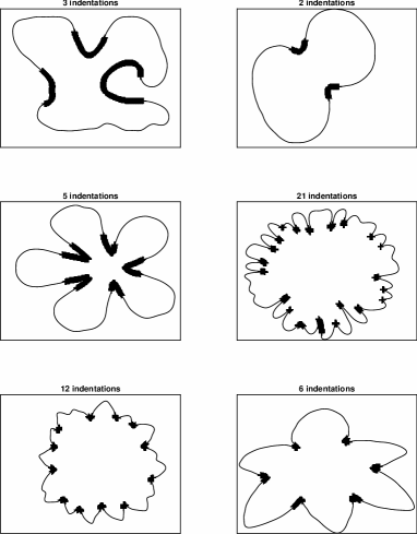
Fig. 3: Demonstration of the algorithm for six test images: two synthetic and four obtained from segmented photographs.

5.2 Comparison with convex hull approaches

A simple approach to solving this same problem using readily available algorithms is to examine the convex hull of the shape and count the number of regions where a gap appears between the convex hull and the curve itself. An example is shown in Figure 4(a), with the blob and its convex hull shown in Figure 4(b). Gaps between the shape and the convex hull can be obtained by subtracting the blob from its convex hull as shown in Figure 4(c). The problem with this approach is that it makes a simplistic assumption about what constitutes an indentation: specifically, that a shape without indentations will strictly match its own convex hull. This is unrealistic in many applications in which non-indentation boundary irregularities are expected. A consequence of this is that some indentations may be missed: a detailed region along the shape boundary is shown in Figure 4(d). Using the calculated curvature along the shape boundary is insensitive to this kind of shape since the curvature analysis makes no assumptions about the shape relative to a canonical analogue such as the convex hull.

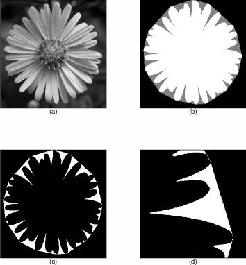
Fig. 4: An example showing indentations missed by examining the difference between the shape and its convex hull.

The attraction of convex hull methods is the ready availability of efficient algorithm implementations. Fortunately, the method presented in this paper also leverages a fundamental algorithm with widespread deployment, the Fast Fourier Transform. As such, the methods described in this paper are competitive in both accessibility as well as algorithmic efficiency since the FFT has time complexity $O(n\log n)$ for $n$ points, comparable to the average time complexity of the QuickHull method ($O(n\log n$) average, $O(n^{2})$ worst-case).

6 Conclusions

In this paper a method has been demonstrated to use the computed curvature along the boundary of a 2D shape to identify indentations. This method is based on calculation of curvature via the Fourier transform and selection of indentations using a single scalar parameter corresponding to the maximum radius of curvature allowed to be considered an indentation. Unlike methods based on the convex hull or piecewise linear polygon approximations, the selection of indentations requires no heuristic tests and cleanly integrates frequency-domain filtering of the shape boundary to eliminate pixel-level discretization effects along the boundary of the shape.

An implementation of this algorithm is available as an open source MATLAB package.

References

- [1] C. Bradford Barber, David P. Dobkin, and Hannu Huhdanpaa, “The quickhull algorithm for convex hulls,” ACM Transactions on Mathematical Software, vol. 22, no. 4, pp. 469–483, 1996.
- [2] Franco P. Preparata and Michael Ian Shamos, Computational Geometry: An Introduction, Springer-Verlag, 1985.
- [3] H. Edelsbrunner, D. Kirkpatrick, and R. Seidel, “On the shape of a set of points in the plane,” Information Theory, IEEE Transactions on, vol. 29, no. 4, pp. 551–559, Jul 1983.
- [4] Herbert Edelsbrunner and John L. Harer, Computational Topology: An Introduction, American Mathematical Society, 2010.
- [5] Tamal K. Dey, Curve and Surface Reconstruction: Algorithms with Mathematical Analysis, Cambridge, 2007.
- [6] Georgi P. Tolstov, Fourier Series, Dover Publications, 1977.
- [7] David W. Henderson, Differential Geometry: A Geometric Introduction, Prentice Hall, 1998.