Radiative transition of negative to positive parity nucleon

We investigate the $N^{\ast}(1535)\rightarrow N\gamma$ transition in the framework of light cone QCD sum rules. In particular, using the most general form of the interpolating current for the nucleon as well as the distribution amplitudes of the photon, we calculate two transition form factors responsible for this channel and use them to evaluate the decay width and branching ratio of the transition under consideration. The result obtained for the branching fraction is in a good consistency with the experimental data.

PACS number(s): 13.40.Gp, 13.30.Ce, 14.20.Dh, 11.55.Hx

1 Introduction

The investigation of the decay properties of hadrons plays essential role in understanding their internal structures as well as the perturbative and non-perturbative aspects of QCD. The theoretical study on the decay channels of the negative parity baryons, especially their radiative transitions, can be more useful in this regard as we have limited information about the decay properties of these states, experimentally. Some experimental studies on the photo-production and electro-production are planned to measure the electromagnetic form factors and multipole moments of the negative parity baryons at Jefferson Laboratory [1] and Mainz Microton facility [2, 3, 4]. One of the main difficulty in measuring the magnetic moments of the excited baryons can be related to the considerably large width that they have. The magnetic moments of these states can be measured from the polarization observables of the decay products of their excited resonances. It is hoped that the new electron beam facilities would allow to collect a large numbers of more precise data in the studies of the electro-excitations of the nucleon resonances.

One of the main directions in obtaining essential information about the internal structure and natures of the negative parity baryons is to study their electromagnetic form factors and multipole moments both theoretically and experimentally. Such studies can also provide valuable information about their geometric shape. In this accordance, in the present study, we investigate the radiative $N^{\ast}(1535)\rightarrow N\gamma$ transition in the framework of light cone QCD sum rules (LCSR), where $N^{\ast}(1535)$ is the low-lying negative parity nucleon with $J^{P}=\frac{1}{2}^{-}$. In the following, we will briefly refer to this state by $N^{\ast}$. In particular, we calculate the two transition form factors $f_{1}^{T}$ and $f_{2}^{T}$ defining this channel (negative parity to positive parity nucleon) separating the contributions of the positive to positive and negative to negative parity transitions entering the physical side of correlation function. In the calculations, we use the most general form of the interpolating currents coupled to both the positive and negative parity nucleons and try to find the working region of the general parameter entering the general interpolating current. We also deal with real photon and calculate the transition form factors at zero transfered momentum squared using the photon distribution amplitudes (DAs). In the following, we shall refer to some studies on the spectroscopic and decay properties of the negative parity baryons. The mass and other spectroscopic properties of the negative parity nucleons have been extensively studied compared to their decays (for instance see [5, 6, 7, 8, 9] and references therein). The light-cone DAs of the nucleon and negative parity nucleon resonances was studied via Lattice QCD in [10]. The magnetic moments of the negative parity baryons have been studied via QCD sum rules in [11] and from effective Hamiltonian approach to QCD in [12]. The $\gamma^{\ast}N\to N(1535)$ and $\gamma^{\ast}N\to N^{\ast}(1520)$ transition form factors are studied in [13, 14] in light cone QCD sum rules using the nucleon DAs. The electromagnetic transitions of the octet negative parity to octet positive parity baryons is also studied in [15] via light cone QCD sum rules.

The layout of the paper is as follows. In next section, we derive LCSR for the transition electromagnetic form factors under consideration. The last section is dedicated to the numerical analysis of the form factors, calculation of the total decay width and branching fraction of the considered radiative transition. We also compare the results obtained with the existing experimental data.

2 LCSR for radiative transition of negative to positive parity nucleon

The aim of this section is to give some details of the calculations of LCSR for the transition form factors defining the radiative $N^{\ast}\rightarrow N\gamma$ channel. To fulfill this aim, we consider the following two-point correlation function in the presence of the background photon field:

$$\Pi=i\int d^{4}x~{}e^{ip\cdot x}~{}{\langle}0|{\cal T}\left(\eta(x)~{}\bar{\eta}(0)~{}\right)|0{\rangle}_{\gamma},$$ (1)

where $\eta$ is the interpolating current coupled to both the negative and positive parity nucleon and ${\cal T}$ denotes the time ordering operator. According to the methodology of QCD sum rule, the calculation of the above mentioned correlation function is made via following two different ways in order to construct sum rules for the transition form factors. In the first way, one calculates it in terms of the hadronic degrees of freedom called as hadronic side. In the second way, it is calculated in terms of photon distribution amplitudes (DAs) with increasing twist by the help of operator product expansion (OPE) called as OPE side. These two sides are then matched to obtain the LCSR for the form factors under consideration. We apply a double Borel transformation with respect to the momentum squared of the initial and final states to both sides to suppress the contributions of the higher states and continuum.

2.1 Hadronic side

The calculation of the hadronic side of the correlation function in Eq. (1) requires its saturation with complete sets of intermediate states having the same quantum numbers as the interpolating current coupling to both the negative and positive parity states. After performing the four-integral over $x$, we get

$$\Pi^{HAD} = \frac{{\langle}0|\eta|N(p,s){\rangle}}{p^{2}-m_{N}^{2}}{\langle}N(p,s)\gamma(q)|N(p+q,s^{\prime}){\rangle}\frac{{\langle}N(p+q,s^{\prime})|\bar{\eta}|0{\rangle}}{(p+q)^{2}-m_{N}^{2}}$$ (2)

$$+ \frac{{\langle}0|\eta|N^{\ast}(p,s){\rangle}}{p^{2}-m_{N^{\ast}}^{2}}{\langle}N^{\ast}(p,s)\gamma(q)|N^{\ast}(p+q,s^{\prime}){\rangle}\frac{{\langle}N^{\ast}(p+q,s^{\prime})|\bar{\eta}|0{\rangle}}{(p+q)^{2}-m_{N^{\ast}}^{2}}$$

$$+ \frac{{\langle}0|\eta|N(p,s){\rangle}}{p^{2}-m_{N}^{2}}{\langle}N(p,s)\gamma(q)|N^{\ast}(p+q,s^{\prime}){\rangle}\frac{{\langle}N^{\ast}(p+q,s^{\prime})|\bar{\eta}|0{\rangle}}{(p+q)^{2}-m_{N^{\ast}}^{2}}$$

$$+ \frac{{\langle}0|\eta|N^{\ast}(p,s){\rangle}}{p^{2}-m_{N^{\ast}}^{2}}{\langle}N^{\ast}(p,s)\gamma(q)|N(p+q,s^{\prime}){\rangle}\frac{{\langle}N(p+q,s^{\prime})|\bar{\eta}|0{\rangle}}{(p+q)^{2}-m_{N}^{2}}$$

$$+ \cdots~{},$$

where $\cdots$ represents the contributions coming from the higher states and continuum. The matrix elements in the above equation can be parameterized in terms of residues $\lambda_{N}$ and $\lambda_{N^{\ast}}$ as well as transition form factors $f_{1}$, $f_{2}$, $f^{*}_{1}$, $f^{*}_{2}$, $f^{T}_{1}$ and $f^{T}_{2}$ at $q^{2}=0$ as

$$\langle 0\mid\eta\mid N(p,s)\rangle = \lambda_{N}u_{N}(p,s),$$

$$\langle N(p+q,s^{\prime})\mid\bar{\eta}\mid 0\rangle = \lambda_{N}\bar{u}_{N}(p+q,s^{\prime}),$$

$$\langle 0\mid\eta\mid N^{\ast}(p,s)\rangle = \lambda_{N^{\ast}}\gamma_{5}u_{N^{\ast}}(p,s),$$

$$\langle N^{\ast}(p+q,s^{\prime})\mid\bar{\eta}\mid 0\rangle = \lambda_{N^{\ast}}\bar{u}_{N^{\ast}}(p+q,s^{\prime})\gamma_{5},$$

$$\langle N(p,s)\gamma(q)\mid N(p+q,s^{\prime})\rangle = e\varepsilon^{\mu}\bar{u}_{N}(p,s)\Big{[}f_{1}\gamma_{\mu}-\frac{i\sigma_{\mu\nu}}{2m_{N}}q^{\nu}f_{2}\Big{]}u_{N}(p+q,s^{\prime}),$$

$$\langle N^{\ast}(p,s)\gamma(q)\mid N^{\ast}(p+q,s^{\prime})\rangle = e\varepsilon^{\mu}\bar{u}_{N^{\ast}}(p,s)\Big{[}f_{1}^{\ast}\gamma_{\mu}-\frac{i\sigma_{\mu\nu}}{2m_{N^{\ast}}}q^{\nu}f_{2}^{\ast}\Big{]}u_{N^{\ast}}(p+q,s^{\prime}),$$

$$\langle N(p,s)\gamma(q)\mid N^{\ast}(p+q,s^{\prime})\rangle = e\varepsilon^{\mu}\bar{u}_{N}(p,s)\Big{[}f_{1}^{T}\gamma_{\mu}-\frac{i\sigma_{\mu\nu}}{m_{N}+m_{N^{\ast}}}q^{\nu}f_{2}^{T}\Big{]}\gamma_{5}u_{N^{\ast}}(p+q,s^{\prime}),$$

$$\langle N^{\ast}(p,s)\gamma(q)\mid N(p+q,s^{\prime})\rangle = e\varepsilon^{\mu}\bar{u}_{N^{\ast}}(p,s)\Big{[}f_{1}^{T}\gamma_{\mu}-\frac{i\sigma_{\mu\nu}}{m_{N}+m_{N^{\ast}}}q^{\nu}f_{2}^{T}\Big{]}\gamma_{5}u_{N}(p+q,s^{\prime}),$$

where $u_{N}$ and $u_{N^{\ast}}$ are the spinors for the positive parity $N$ and negative parity $N^{\ast}$ nucleons, respectively. The use of Eq. (2.1) into Eq. (2) is followed by summing over the spins of the $N$ and $N^{\ast}$ baryons, i.e.

$$\sum_{s}u_{N^{(*)}}(p,s)\bar{u}_{N^{(*)}}(p,s) = \not\!p+m_{N^{(*)}}~{}.$$ (4)

As a result, we have

$$\Pi^{HAD} = \frac{\lambda_{N}^{2}~{}e}{(p^{2}-m_{N}^{2})[(p+q)^{2}-m_{N}^{2}]}(\not\!p+m_{N})\Big{[}(f_{1}+f_{2})\not\!\varepsilon-\frac{p\cdot\varepsilon}{m_{N}}f_{2}\Big{]}(\not\!p+\not\!q+m_{N})$$ (5)

$$+ \frac{\lambda_{N^{\ast}}^{2}~{}e}{(p^{2}-m_{N^{\star}}^{2})[(p+q)^{2}-m_{N^{\ast}}^{2}]}(-\not\!p+m_{N^{\ast}})\Big{[}-(f_{1}^{\ast}+f_{2}^{\ast})\not\!\varepsilon-\frac{p\cdot\varepsilon}{m_{N^{\ast}}}f_{2}^{\ast}\Big{]}(-\not\!p-\not\!q+m_{N^{\ast}})$$

$$+ \frac{\lambda_{N}\lambda_{N^{\ast}}~{}e}{(p^{2}-m_{N}^{2})[(p+q)^{2}-m_{N^{\ast}}^{2}]}(\not\!p+m_{N})\Big{[}(f_{1}^{T}-\frac{m_{N^{\ast}}-m_{N}}{m_{N^{\ast}}+m_{N}}f_{2}^{T})\not\!\varepsilon-\frac{2p\cdot\varepsilon}{m_{N^{\ast}}+m_{N}}f_{2}^{T}\Big{]}$$

$$\times (-\not\!p-\not\!q+m_{N^{\ast}})$$

$$+ \frac{\lambda_{N}\lambda_{N^{\ast}}~{}e}{(p^{2}-m_{N^{\ast}}^{2})[(p+q)^{2}-m_{N}^{2}]}(-\not\!p+m_{N^{\ast}})\Big{[}-(f_{1}^{T}+\frac{m_{N^{\ast}}-m_{N}}{m_{N^{\ast}}+m_{N}}f_{2}^{T})\not\!\varepsilon-\frac{2p\cdot\varepsilon}{m_{N^{\ast}}+m_{N}}f_{2}^{T}\Big{]}$$

$$\times (\not\!p+\not\!q+m_{N})$$

$$+ \cdots~{}.$$

Our aim in the present study is to calculate the transition form factors $f_{1}^{T}$ and $f_{2}^{T}$ defining the radiative $N^{\ast}\rightarrow N\gamma$ transition. For this purpose, we use the structures $\not\!p\not\!\varepsilon\not\!q$, $\not\!p\not\!\varepsilon$, $\not\!\varepsilon\not\!q$ and $\not\!\varepsilon$ in our calculations. The final form of the hadronic side of the correlation function is obtained after the application of a double Borel transformation with respect to the initial and final momenta squared, viz.

$$\widehat{\textbf{B}}\Pi^{HAD} = \Pi_{1}^{HAD}\not\!p\not\!\varepsilon\not\!q+\Pi_{2}^{HAD}\not\!p\not\!\varepsilon+\Pi_{3}^{HAD}\not\!\varepsilon\not\!q+\Pi_{4}^{HAD}\not\!\varepsilon+\cdots~{},$$ (6)

where we have kept only the structures which we use to construct the LCSR for the form factors under consideration. The functions $\Pi_{i=1,2,3,4}^{HAD}$ are obtained as

$$\Pi_{1}^{HAD} = \frac{2e\lambda_{N}\lambda_{N^{\ast}}(m_{N^{\ast}}-m_{N})}{m_{N}+m_{N^{\ast}}}f_{2}^{T}e^{-\frac{m_{N^{\ast}}^{2}}{M_{1}^{2}}-\frac{m_{N}^{2}}{M_{2}^{2}}}+e\lambda_{N}^{2}\mu_{N}e^{-\frac{2m_{N}^{2}}{M_{2}^{2}}}-e\lambda_{N^{\ast}}^{2}\mu_{N^{\ast}}e^{-\frac{2m_{N^{\ast}}^{2}}{M_{1}^{2}}},$$

$$\Pi_{2}^{HAD} = 2e\lambda_{N}\lambda_{N^{\ast}}(m_{N}+m_{N^{\ast}})f_{1}^{T}e^{-\frac{m_{N^{\ast}}^{2}}{M_{1}^{2}}-\frac{m_{N}^{2}}{M_{2}^{2}}},$$

$$\Pi_{3}^{HAD} = -\frac{e\lambda_{N}\lambda_{N^{\ast}}[f_{1}^{T}(m_{N^{\ast}}+m_{N})^{2}+f_{2}^{T}(m_{N^{\ast}}-m_{N})^{2}]}{m_{N}+m_{N^{\ast}}}e^{-\frac{m_{N^{\ast}}^{2}}{M_{1}^{2}}-\frac{m_{N}^{2}}{M_{2}^{2}}}$$

$$+ e\lambda_{N}^{2}\mu_{N}m_{N}e^{-\frac{2m_{N}^{2}}{M_{2}^{2}}}+e\lambda_{N^{\ast}}^{2}\mu_{N^{\ast}}m_{N^{\ast}}e^{-\frac{2m_{N^{\ast}}^{2}}{M_{1}^{2}}},$$

$$\Pi_{4}^{HAD} = -e\lambda_{N}\lambda_{N^{\ast}}(m_{N^{\ast}}^{2}-m_{N}^{2})(f_{1}^{T}+f_{2}^{T})e^{-\frac{m_{N^{\ast}}^{2}}{M_{1}^{2}}-\frac{m_{N}^{2}}{M_{2}^{2}}},$$ (7)

where $M_{1}^{2}$ and $M_{2}^{2}$ are Borel mass parameters. As it is clear from the explicit forms of the functions $\Pi_{i}^{HAD}$, they also include the magnetic moments $\mu_{N}=f_{1}+f_{2}$ and $\mu_{N^{\ast}}=f_{1}^{\ast}+f_{2}^{\ast}$ which are calculated in [16] and [11], respectively.

2.2 OPE Side

The OPE side of the correlation function is calculated in terms of the QCD parameters and photon DAs. To this aim we need to know the explicit form of the nucleon interpolating current coupling to both the negative and positive parity state. It is given as

$$\eta=2\varepsilon^{abc}\Big{\{}\Big{(}u^{aT}Cd^{b}\Big{)}\gamma_{5}u^{c}+\beta\Big{(}u^{aT}C\gamma_{5}d^{b}\Big{)}u^{c}\Big{\}},$$ (8)

where $a$, $b$ and $c$ are color indices and $C$ is the charge conjugation operator. The parameter $\beta$ is a general mixing parameter, which we shall find its working region in next section. We insert the aforementioned interpolating current into the correlation function in Eq. (1) and use the Wick’s theorem to contract out all the quark pairs. This leads to obtain the correlation function on OPE side in terms of the light quark propagators.

The correlation function in OPE side contains three different parts:

• perturbative part,

• mixed part at which the photon is radiated from short distances and at least one of the quarks interacts with the QCD vacuum and makes a condensate,

• non-perturbative part at which the photon is radiated at long distances. This contribution appears as the matrix elements $\langle\gamma(q)\mid\bar{q}(x_{1})\Gamma q(x_{2})\mid 0\rangle$, which are expressed in terms of the photon DAs having distinct twists. The $\Gamma$ appearing in this matrix element refers to the full set of Dirac matrices, namely $\Gamma_{j}=\Big{\{}1,~{}\gamma_{5},~{}\gamma_{\alpha},~{}i\gamma_{5}\gamma_{\alpha},~{}\sigma_{\alpha\beta}/\sqrt{2}\Big{\}}$.

The perturbative contributions where the photon perturbatively interacts with the quarks are acquired via replacing the corresponding free light quark propagator with

$$S^{ab}_{\alpha\beta}\Rightarrow\left\{\int d^{4}yS^{free}(x-y)\not\!AS^{free}(y)\right\}^{ab}_{\alpha\beta},$$ (9)

at which the free part of the light quark propagator is written as

$$S^{free}_{q} = \frac{i\not\!x}{2\pi^{2}x^{4}}-\frac{m_{q}}{4\pi^{2}x^{2}},$$

where $q$ stands for the light $u$ or $d$ quark.

To obtain the non-perturbative contributions we replace the light quark propagator that interacts with the photon with

$$S^{ab}_{\alpha\beta}\rightarrow-\frac{1}{4}\bar{q}^{a}\Gamma_{j}q^{b}(\Gamma_{j})_{\alpha\beta}~{}.$$ (11)

The remaining quark propagators are replaced with the full quark propagators which include all the perturbative and non-perturbative parts. The full light quark propagator is given as [17, 18]

$$S_{q}(x) = S_{q}^{free}(x)-\frac{m_{q}}{4\pi^{2}x^{2}}-\frac{\langle\bar{q}q\rangle}{12}\left(1-i\frac{m_{q}}{4}\not\!x\right)-\frac{x^{2}}{192}m_{0}^{2}\langle\bar{q}q\rangle\left(1-i\frac{m_{q}}{6}\not\!x\right)$$ (12)

$$-ig_{s}\int_{0}^{1}du\left[\frac{\not\!x}{16\pi^{2}x^{2}}G_{\mu\nu}(ux)\sigma_{\mu\nu}-ux^{\mu}G_{\mu\nu}(ux)\gamma^{\nu}\frac{i}{4\pi^{2}x^{2}}\right.$$

$$\left.-i\frac{m_{q}}{32\pi^{2}}G_{\mu\nu}\sigma^{\mu\nu}\left(\ln\left(\frac{-x^{2}\Lambda^{2}}{4}\right)+2\gamma_{E}\right)\right],$$

where $\Lambda$ is a scale parameter.

As it has already mentioned, in calculations of the non-perturbative contributions, there appear matrix elements like $\langle\gamma(q)\mid\bar{q}\Gamma_{i}q\mid 0\rangle$. These matrix elements are expanded in terms of the photon DAs with increasing twists. We present the parametrization of these matrix elements in terms of the photon DAs together with the explicit forms of the photon wave functions as well as the related parameters in the Appendix. After very lengthy calculations, we obtain the OPE side of the correlation function in momentum space in terms of the photon DAs and other QCD parameters. The final form of the OPE side of the correlation function is obtained by applying a Borel transformation with respect to the variables $p^{2}$ and $(p+q)^{2}$.

Having calculated both the hadronic and OPE sides of the correlation function in Borel scheme it is the time for matching the two sides in order to obtain LCSR for the transition form factors $f_{1}^{T}$ and $f_{2}^{T}$, defining the radiative transition under consideration. For this purpose, we match the coefficients of the structures $\not\!p\not\!\varepsilon\not\!q$, $\not\!p\not\!\varepsilon$, $\not\!\varepsilon\not\!q$ and $\not\!\varepsilon$ from both sides of the correlation function. To further suppress the contributions of the higher states and continuum we also perform continuum subtraction. By simultaneous solving of four equations obtained via matching the coefficients of the above structures from both the hadronic and OPE sides, we get the following sum rules for the form factors under consideration:

$$f_{1}^{T} = \frac{1}{2e\lambda_{N}\lambda_{N^{\ast}}(m_{N}+m_{N^{\ast}})}e^{\frac{m_{N}^{2}}{M_{2}^{2}}+\frac{m_{N^{\ast}}^{2}}{M_{1}^{2}}}\Pi_{2}^{OPE}(M^{2},s_{0},\beta,u_{0})$$

$$f_{2}^{T} = \frac{1}{2e\lambda_{N}\lambda_{N^{\ast}}(m_{N}^{2}-m_{N^{\ast}}^{2})}e^{\frac{m_{N}^{2}}{M_{2}^{2}}+\frac{m_{N^{\ast}}^{2}}{M_{1}^{2}}}\Big{[}\Pi_{2}^{OPE}(M^{2},s_{0},\beta,u_{0})\Big{(}m_{N^{\ast}}-m_{N}\Big{)}$$

$$+ 2\Pi_{4}^{OPE}~{}(M^{2},s_{0},\beta,u_{0})\Big{]},$$

where $s_{0}$ is the continuum threshold and the functions $\Pi_{i}^{OPE}(M^{2},s_{0},\beta,u_{0})$ are very lengthy, so we do not present their explicit forms here. In the above equation, $u_{0}$ and the new Borel parameter $M^{2}$ are obtained in terms of the Borel parameters $M_{1}^{2}$ and $M_{2}^{2}$ as

$$u_{0} = \frac{M_{1}^{2}}{M_{1}^{2}+M_{2}^{2}},$$

$$M^{2} = \frac{M_{1}^{2}M_{2}^{2}}{M_{1}^{2}+M_{2}^{2}}.$$ (14)

Using the relation $\frac{M_{1}^{2}}{M_{2}^{2}}\simeq\frac{m_{N^{\ast}}^{2}}{m_{N}^{2}}$, we obtain $M_{1}^{2}$ and $M_{2}^{2}$ in terms of $M^{2}$ as

$$M_{1}^{2} = \frac{m_{N}^{2}+m_{N^{\ast}}^{2}}{m_{N}^{2}}M^{2},$$

$$M_{2}^{2} = \frac{m_{N}^{2}+m_{N^{\ast}}^{2}}{m_{N^{\ast}}^{2}}M^{2}.$$ (15)

We also obtain $u_{0}$ in terms of the masses of the positive and negative parity baryons as

$$u_{0} = \frac{m_{N^{\ast}}^{2}}{m_{N}^{2}+m_{N^{\ast}}^{2}},$$ (16)

at which we calculate the photon wave functions and the related integrals.

As it is clear from Eq. (2.2), to extract the values of the form factors $f_{1}^{T}$ and $f_{2}^{T}$ we need to know the residues of both the negative and positive parity nucleons. They are calculated using a two-point correlation function, viz.

$$\Pi^{\prime}=i\int d^{4}x~{}e^{ip\cdot x}~{}{\langle}0|{\cal T}\left(\eta(x)~{}\bar{\eta}(0)~{}\right)|0{\rangle}.$$ (17)

This function also is calculated via two different ways, namely via hadronic and OPE languages. The hadronic side of this correlation function including both the negative and positive parity nucleons is obtained as

$$\Pi^{\prime HAD}=\frac{{\langle}0|\eta|N(p,s){\rangle}{\langle}N(p,s)|\bar{\eta}|0{\rangle}}{m_{N}^{2}-p^{2}}+\frac{{\langle}0|\eta|N^{\ast}(p,s){\rangle}{\langle}N^{\ast}(p,s)|\bar{\eta}|0{\rangle}}{m_{N^{\ast}}^{2}-p^{2}}+....$$ (18)

By using the definitions of the residues from Eq. (2.1) and summing over the spins of the baryons $N$ and $N^{\ast}$ and applying the Borel transformation, we obtain the final form of the hadronic side of the correlation function in the Borel scheme as

$$\widehat{\textbf{B}}\Pi^{\prime HAD}=|\lambda_{N}^{2}|e^{-m_{N}^{2}/M^{\prime^{2}}}\Big{(}\not\!p+m_{N}U\Big{)}+|\lambda_{N^{\ast}}^{2}|e^{-m_{N^{\ast}}^{2}/M^{\prime^{2}}}\Big{(}-\not\!p+m_{N^{\ast}}U\Big{)},$$ (19)

where $U$ is the unit matrix and $M^{\prime^{2}}$ is the Borel mass parameters in the mass sum rule. The OPE side of the above correlation function is also calculated in deep Euclidean region in terms of QCD degrees of freedom and the structures $\not\!p$ and $U$, i.e.

$$\widehat{\textbf{B}}\Pi^{\prime OPE}=\Pi^{\prime OPE}_{1}(M^{\prime^{2}},s^{\prime}_{0},\beta)\not\!p+\Pi^{\prime OPE}_{2}(M^{\prime^{2}},s^{\prime}_{0},\beta)U,$$ (20)

where $s^{\prime}_{0}$ is the continuum threshold in the mass sum rule. Then we match again the coefficients of the selected structures from both sides. By simultaneous solving of the two appeared equations, we get the following sum rules for the residues of $N$ and $N^{\ast}$ nucleons in terms of their masses and other parameters:

$$|\lambda_{N}^{2}|=\frac{e^{m_{N}^{2}/M^{\prime^{2}}}}{m_{N}+m_{N^{\ast}}}\Big{[}m_{N^{\ast}}\Pi^{\prime OPE}_{1}(M^{\prime^{2}},s^{\prime}_{0},\beta)+\Pi^{\prime OPE}_{2}(M^{\prime^{2}},s^{\prime}_{0},\beta)\Big{]},$$

$$|\lambda_{N^{\ast}}^{2}|=\frac{e^{m_{N^{\ast}}^{2}/M^{\prime^{2}}}}{m_{N}+m_{N^{\ast}}}\Big{[}-m_{N}\Pi^{\prime OPE}_{1}(M^{\prime^{2}},s^{\prime}_{0},\beta)+\Pi^{\prime OPE}_{2}(M^{\prime^{2}},s^{\prime}_{0},\beta)\Big{]}.$$ (21)

Here we should also stress that the functions $\Pi^{\prime OPE}_{1}(M^{\prime^{2}},s^{\prime}_{0},\beta)$ and $\Pi^{\prime OPE}_{2}(M^{\prime^{2}},s^{\prime}_{0},\beta)$ have very lengthy expressions and for this reason we do not present their explicit forms.

3 Numerical results

First of all we would like to obtain the behaviors of the residues of the positive and negative parity baryons with respect to the general parameter $\beta$ entering the general form of the interpolating current discussed in the previous section. To this aim we use some input parameters $\langle\bar{u}u\rangle=\langle\bar{d}d\rangle=-(0.243)^{3}~{}GeV^{3}$, $\langle\bar{s}s\rangle=0.8\langle\bar{u}u\rangle$ and $m_{0}^{2}=(0.8\pm 0.2)~{}GeV^{2}$ [19]. Beside these, we need also to find the working regions of auxiliary parameters $M^{\prime^{2}}$, $s^{\prime}_{0}$ and $\beta$ entering the sum rules for the residues. The general criteria in the sum rule method is that the physical quantities are practically independent of the auxiliary parameters, hence, we look for some regions of these helping parameters such that the residues weakly depend of them in these regions. The continuum threshold depends on the energy of the first excited state with the same quantum numbers as the interpolating current for both the negative and positive parity states. Our calculations show that in the intervals

$$1.08\,GeV^{2}\leq s_{0}^{\prime} \leq 1.98\,GeV^{2}\,\,\,\,\,\mbox{for}\,\,\,\,\,N,$$

and

$$2.51\,GeV^{2}\leq s_{0}^{\prime} \leq 2.73\,GeV^{2}\,\,\,\,\,\mbox{for}\,\,\,\,\,N^{\ast},$$ (22)

the residues weakly depend on the continuum threshold. The working region of the Borel mass parameter $M^{\prime^{2}}$ is obtained demanding that not only the perturbative contributions to the residues exceed the non-perturbative ones but also the operators with higher dimensions have small contributions compared to the lower dimensional operators. This leads to the Borel windows

$$0.5\,GeV^{2}\leq M^{\prime^{2}} \leq 1.5\,GeV^{2}\,\,\,\,\,\mbox{for}\,\,\,\,\,N,$$

and

$$2\,GeV^{2}\leq M^{\prime^{2}} \leq 4\,GeV^{2}\,\,\,\,\,\mbox{for}\,\,\,\,\,N^{\ast}.$$ (23)

It is also found that in the intervals $-0.60\leq\cos\theta\leq-0.30$ and $0.30\leq\cos\theta\leq 0.60$ for $N$ as well as $-0.62\leq\cos\theta\leq-0.30$ for $N^{\ast}$, at which $\theta=tan^{-1}\beta$, the residues have relatively weak dependency on the general parameter $\beta$. Using these working windows for the auxiliary parameters as well as other inputs we find that the residue squares as functions of the general parameter $\beta$ in the positive and negative parity channels can be parametrized as

$$\lambda_{N}^{2}(\beta) = e^{\frac{m_{N}^{2}}{M^{\prime^{2}}}}\Phi_{1}(\beta),$$

$$\lambda_{N^{\ast}}^{2}(\beta) = e^{\frac{m_{N^{\ast}}^{2}}{M^{\prime^{2}}}}\Phi_{2}(\beta),$$ (24)

where

$$\Phi_{1}(\beta) = [2.28-3.20\beta+64.10\beta^{2}]\times 10^{-6}~{}~{}(GeV^{6}),$$

$$\Phi_{2}(\beta) = [-7.38-4.20\beta+2.82\beta^{2}]\times 10^{-5}~{}~{}(GeV^{6}).$$ (25)

Now, we perform numerical analysis of the sum rules for the transition form factors and use them to predict the decay width and branching ratio of the radiative $N^{\ast}\rightarrow N\gamma$ transition. To this aim, we need the photon DAs and wave functions as well as the corresponding parameters, which are given in the Appendix. Beside these inputs and the residues obtained above in terms of the general parameter $\beta$, we also need the parameters $f_{3\gamma}=-0.0039~{}GeV^{2}$ [20] and $\chi(1~{}GeV)=-4.4~{}GeV^{-2}$ [21].

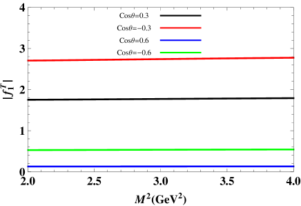
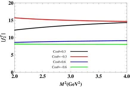
The sum rules for the form factors $f_{1}^{T}$ and $f_{2}^{T}$, contain three more auxiliary parameters: the Borel mass parameter $M^{2}$, the continuum threshold $s_{0}$ and the arbitrary parameter $\beta$ entering the expression of the interpolating current. The working window for $M^{2}$ is obtained requiring that not only the ground state contribution exceeds the contributions of the higher states and continuum but the contributions of the leading twists exceed those of the higher twists, i.e., the series of the sum rules for the form factors converge. These requirements lead to the interval $2~{}GeV^{2}\leq M^{2}\leq 4~{}GeV^{2}$. We also choose the interval $2.51~{}GeV^{2}\leq s_{0}\leq 2.73~{}GeV^{2}$ for the continuum threshold, at which the dependence of the form factors on this parameter are weak. Our numerical calculations also lead to the working regions $-0.60\leq\cos\theta\leq-0.30$ and $0.30\leq\cos\theta\leq 0.60$ for the arbitrary parameter $\beta=\tan\theta$. We depict the dependence of the form factors $f_{1}^{T}$ and $f_{2}^{T}$ on the Borel mass parameters $M^{2}$ at fixed value of $s_{0}$ and different values of $\cos\theta$ in figure 1. With a quick glance at this figure, we see that these form factors depict weak dependence on the Borel parameter on its working regions.

Figure 1: Left: The dependence of the form factor $f_{1}^{T}$ for $N^{\ast}\rightarrow N\gamma$ transition on the Borel mass parameter $M^{2}$ at $s_{0}=2.67~{}GeV^{2}$ and different values of $\cos\theta$. Right: The dependence of the form factor $f_{2}^{T}$ for $N^{\ast}\rightarrow N\gamma$ transition on the Borel mass parameter $M^{2}$ at $s_{0}=2.67~{}GeV^{2}$ and different values of $\cos\theta$.

Using all input parameters and working regions of all auxiliary parameters as well as the masses and residues of the negative and positive parity baryons obtained via mass sum rules, the average values of the transition form factors $f_{1}^{T}$ and $f_{2}^{T}$ for the $N^{\ast}\rightarrow N\gamma$ channel are obtained as presented in table 1.

$$\begin{array}[]{|c|c|}\hline\cr\hline\cr\mbox{$f_{1}^{T}$}&1.26\pm 0.37\\ \hline\cr\mbox{$f_{2}^{T}$}&11.18\pm 3.35\\ \hline\cr\hline\cr\end{array}$$

Table 1: The values of the form factors $f_{1}^{T}$ and $f_{2}^{T}$ for the $N^{\ast}\rightarrow N\gamma$ transition.

At the end of this section, we would like to calculate the decay width for the radiative $N^{\ast}\rightarrow N\gamma$ transition. Considering the corresponding transition matrix elements in Eq. (2.1), we obtain the following formula for the total width of the transition under consideration:

$$\Gamma = \frac{\alpha_{em}}{2m_{N^{\ast}}^{3}}\Big{(}m_{N}^{2}-m_{N^{\ast}}^{2}\Big{)}\Bigg{\{}|f_{1}^{T}|^{2}\Big{(}m_{N}^{2}+4m_{N}m_{N^{\ast}}+m_{N^{\ast}}^{2}\Big{)}-3Re(f_{1}^{T}f_{2}^{T})\Big{(}m_{N^{\ast}}^{2}-m_{N}^{2}\Big{)}$$ (26)

$$+ |f_{2}^{T}|^{2}\Big{(}m_{N^{\ast}}-m_{N}\Big{)}^{2}\Bigg{\}}.$$

Using the numerical values for the form factors and other input parameters together with the width of the $N^{*}$ state [22], we obtain the numerical values for the decay width and branching ratio of the radiative $N^{\ast}\rightarrow N\gamma$ transition as presented in table 2. In comparison, we also depict the existing related experimental data in this table. Looking at this table we see that our prediction for the branching fraction of the considered transition is in a very good consistency with the experimental data.

$$\begin{array}[]{|c|c|c|}\hline\cr\hline\cr\mbox{}&\Gamma(GeV)&Br\\ \hline\cr\mbox{Present work}&(3.08\pm 0.09)\times 10^{-4}&(0.21\pm 0.06)\times 10^{-2}\\ \hline\cr\mbox{PDG\cite[cite]{[\@@bibref{}{PDG}{}{}]}}&-&(0.15-0.30)\%\\ \hline\cr\hline\cr\end{array}$$

Table 2: Decay width and branching ratio of the radiative $N^{\ast}\rightarrow N\gamma$ transition.

In summary, we have calculated the transition form factors responsible for the radiative transition of negative to positive parity nucleon in the frame work of the LCSR using the most general for of the interpolating current coupling to both the negative and positive parity nucleons as well as the photon DAs. We found the working regions of all auxiliary parameters and obtained the behavior of the residues in terms of the general mixing parameter entering the interpolating current. We used them to predict the numerical values of the form factors for the real photon. The values of the transition form factors are then used to estimate the decay width and branching fraction of the transition under consideration. Our result on the branching ratio of the radiative $N^{\ast}\rightarrow N\gamma$ transition is in a good agreement with the existing experimental data.

4 Acknowledgment

This work has been supported in part by the Scientific and Technological Research Council of Turkey (TUBITAK) under the research project 114F018.

Appendix

The matrix elements appearing in our calculations parametrized in terms of the photon DAs are written as (see [20]) :

$$\langle\gamma(q)|\bar{q}(x)\sigma_{\mu\nu}q(0)|0\rangle=-ie_{q}\bar{q}q(\varepsilon_{\mu}q_{\nu}-\varepsilon_{\nu}q_{\mu})\int_{0}^{1}due^{i\bar{u}qx}\left(\chi\varphi_{\gamma}(u)+\frac{x^{2}}{16}\mathbb{A}(u)\right)$$

$$-\frac{i}{2(qx)}e_{q}\langle\bar{q}q\rangle\left[x_{\nu}\left(\varepsilon_{\mu}-q_{\mu}\frac{\varepsilon x}{qx}\right)-x_{\mu}\left(\varepsilon_{\nu}-q_{\nu}\frac{\varepsilon x}{qx}\right)\right]\int_{0}^{1}due^{i\bar{u}qx}h_{\gamma}(u),$$

$$\langle\gamma(q)|\bar{q}(x)\gamma_{\mu}q(0)|0\rangle=e_{q}f_{3\gamma}\left(\varepsilon_{\mu}-q_{\mu}\frac{\varepsilon x}{qx}\right)\int_{0}^{1}due^{i\bar{u}qx}\psi^{v}(u),$$

$$\langle\gamma(q)|\bar{q}(x)\gamma_{\mu}\gamma_{5}q(0)|0\rangle=-\frac{1}{4}e_{q}f_{3\gamma}\epsilon_{\mu\nu\alpha\beta}\varepsilon^{\nu}q^{\alpha}x^{\beta}\int_{0}^{1}due^{i\bar{u}qx}\psi^{a}(u),$$

$$\langle\gamma(q)|\bar{q}(x)g_{s}G_{\mu\nu}(vx)q(0)|0\rangle=-ie_{q}\langle\bar{q}q\rangle\left(\varepsilon_{\mu}q_{\nu}-\varepsilon_{\nu}q_{\mu}\right)\int{\cal D}\alpha_{i}e^{i(\alpha_{\bar{q}}+v\alpha_{g})qx}{\cal S}(\alpha_{i}),$$

$$\langle\gamma(q)|\bar{q}(x)g_{s}\tilde{G}_{\mu\nu}i\gamma_{5}(vx)q(0)|0\rangle=-ie_{q}\langle\bar{q}q\rangle\left(\varepsilon_{\mu}q_{\nu}-\varepsilon_{\nu}q_{\mu}\right)\int{\cal D}\alpha_{i}e^{i(\alpha_{\bar{q}}+v\alpha_{g})qx}\tilde{\cal S}(\alpha_{i}),$$

$$\langle\gamma(q)|\bar{q}(x)g_{s}\tilde{G}_{\mu\nu}(vx)\gamma_{\alpha}\gamma_{5}q(0)|0\rangle=e_{q}f_{3\gamma}q_{\alpha}(\varepsilon_{\mu}q_{\nu}-\varepsilon_{\nu}q_{\mu})\int{\cal D}\alpha_{i}e^{i(\alpha_{\bar{q}}+v\alpha_{g})qx}{\cal A}(\alpha_{i}),$$

$$\langle\gamma(q)|\bar{q}(x)g_{s}G_{\mu\nu}(vx)i\gamma_{\alpha}q(0)|0\rangle=e_{q}f_{3\gamma}q_{\alpha}(\varepsilon_{\mu}q_{\nu}-\varepsilon_{\nu}q_{\mu})\int{\cal D}\alpha_{i}e^{i(\alpha_{\bar{q}}+v\alpha_{g})qx}{\cal V}(\alpha_{i}),$$

$$\langle\gamma(q)|\bar{q}(x)\sigma_{\alpha\beta}g_{s}G_{\mu\nu}(vx)q(0)|0\rangle=e_{q}\langle\bar{q}q\rangle\left\{\left[\left(\varepsilon_{\mu}-q_{\mu}\frac{\varepsilon x}{qx}\right)\left(g_{\alpha\nu}-\frac{1}{qx}(q_{\alpha}x_{\nu}+q_{\nu}x_{\alpha})\right)\right.\right.q_{\beta}$$

$$-\left(\varepsilon_{\mu}-q_{\mu}\frac{\varepsilon x}{qx}\right)\left(g_{\beta\nu}-\frac{1}{qx}(q_{\beta}x_{\nu}+q_{\nu}x_{\beta})\right)q_{\alpha}$$

$$-\left(\varepsilon_{\nu}-q_{\nu}\frac{\varepsilon x}{qx}\right)\left(g_{\alpha\mu}-\frac{1}{qx}(q_{\alpha}x_{\mu}+q_{\mu}x_{\alpha})\right)q_{\beta}$$

$$+\left.\left(\varepsilon_{\nu}-q_{\nu}\frac{\varepsilon x}{q.x}\right)\left(g_{\beta\mu}-\frac{1}{qx}(q_{\beta}x_{\mu}+q_{\mu}x_{\beta})\right)q_{\alpha}\right]\int{\cal D}\alpha_{i}e^{i(\alpha_{\bar{q}}+v\alpha_{g})qx}{\cal T}_{1}(\alpha_{i})$$

$$+\left[\left(\varepsilon_{\alpha}-q_{\alpha}\frac{\varepsilon x}{qx}\right)\left(g_{\mu\beta}-\frac{1}{qx}(q_{\mu}x_{\beta}+q_{\beta}x_{\mu})\right)\right.q_{\nu}$$

$$-\left(\varepsilon_{\alpha}-q_{\alpha}\frac{\varepsilon x}{qx}\right)\left(g_{\nu\beta}-\frac{1}{qx}(q_{\nu}x_{\beta}+q_{\beta}x_{\nu})\right)q_{\mu}$$

$$-\left(\varepsilon_{\beta}-q_{\beta}\frac{\varepsilon x}{qx}\right)\left(g_{\mu\alpha}-\frac{1}{qx}(q_{\mu}x_{\alpha}+q_{\alpha}x_{\mu})\right)q_{\nu}$$

$$+\left.\left(\varepsilon_{\beta}-q_{\beta}\frac{\varepsilon x}{qx}\right)\left(g_{\nu\alpha}-\frac{1}{qx}(q_{\nu}x_{\alpha}+q_{\alpha}x_{\nu})\right)q_{\mu}\right]\int{\cal D}\alpha_{i}e^{i(\alpha_{\bar{q}}+v\alpha_{g})qx}{\cal T}_{2}(\alpha_{i})$$

$$+\frac{1}{qx}(q_{\mu}x_{\nu}-q_{\nu}x_{\mu})(\varepsilon_{\alpha}q_{\beta}-\varepsilon_{\beta}q_{\alpha})\int{\cal D}\alpha_{i}e^{i(\alpha_{\bar{q}}+v\alpha_{g})qx}{\cal T}_{3}(\alpha_{i})$$

$$+\left.\frac{1}{qx}(q_{\alpha}x_{\beta}-q_{\beta}x_{\alpha})(\varepsilon_{\mu}q_{\nu}-\varepsilon_{\nu}q_{\mu})\int{\cal D}\alpha_{i}e^{i(\alpha_{\bar{q}}+v\alpha_{g})qx}{\cal T}_{4}(\alpha_{i})\right\},$$ (27)

where $\varphi_{\gamma}(u)$ is the leading twist-2 photon DAs, the photon DAs’ $\psi^{v}(u)$, $\psi^{a}(u)$, ${\cal A}(\alpha_{i})$ and ${\cal V}(\alpha_{i})$ have twist 3; and $h_{\gamma}(u)$, $\mathbb{A}$(u) and ${\cal T}_{i}$ ($i=1,~{}2,~{}3,~{}4$) have twist 4 [20]. In the above relations $\chi$ is the magnetic susceptibility of the light quarks.

The measure $\int{\cal D}\alpha_{i}$ entering the calculations is defined as

$$\int{\cal D}\alpha_{i}=\int_{0}^{1}d\alpha_{\bar{q}}\int_{0}^{1}d\alpha_{q}\int_{0}^{1}d\alpha_{g}\delta(1-\alpha_{\bar{q}}-\alpha_{q}-\alpha_{g}).\\$$

The above mentioned photon DAs are also parametrized as [20]:

$$\varphi_{\gamma}(u) = 6u\bar{u}\left(1+\varphi_{2}(\mu)C_{2}^{\frac{3}{2}}(u-\bar{u})\right),$$

$$\psi^{v}(u) = 3\left(3(2u-1)^{2}-1\right)+\frac{3}{64}\left(15w^{V}_{\gamma}-5w^{A}_{\gamma}\right)\left(3-30(2u-1)^{2}+35(2u-1)^{4}\right),$$

$$\psi^{a}(u) = \left(1-(2u-1)^{2}\right)\left(5(2u-1)^{2}-1\right)\frac{5}{2}\left(1+\frac{9}{16}w^{V}_{\gamma}-\frac{3}{16}w^{A}_{\gamma}\right),$$

$${\cal A}(\alpha_{i}) = 360\alpha_{q}\alpha_{\bar{q}}\alpha_{g}^{2}\left(1+w^{A}_{\gamma}\frac{1}{2}(7\alpha_{g}-3)\right),$$

$${\cal V}(\alpha_{i}) = 540w^{V}_{\gamma}(\alpha_{q}-\alpha_{\bar{q}})\alpha_{q}\alpha_{\bar{q}}\alpha_{g}^{2},$$

$$h_{\gamma}(u) = -10\left(1+2\kappa^{+}\right)C_{2}^{\frac{1}{2}}(u-\bar{u}),$$

$$\mathbb{A}(u) = 40u^{2}\bar{u}^{2}\left(3\kappa-\kappa^{+}+1\right)$$

$$+8(\zeta_{2}^{+}-3\zeta_{2})\left[u\bar{u}(2+13u\bar{u})\right.$$

$$+\left.2u^{3}(10-15u+6u^{2})\ln(u)+2\bar{u}^{3}(10-15\bar{u}+6\bar{u}^{2})\ln(\bar{u})\right],$$

$${\cal T}_{1}(\alpha_{i}) = -120(3\zeta_{2}+\zeta_{2}^{+})(\alpha_{\bar{q}}-\alpha_{q})\alpha_{\bar{q}}\alpha_{q}\alpha_{g},$$

$${\cal T}_{2}(\alpha_{i}) = 30\alpha_{g}^{2}(\alpha_{\bar{q}}-\alpha_{q})\left((\kappa-\kappa^{+})+(\zeta_{1}-\zeta_{1}^{+})(1-2\alpha_{g})+\zeta_{2}(3-4\alpha_{g})\right),$$

$${\cal T}_{3}(\alpha_{i}) = -120(3\zeta_{2}-\zeta_{2}^{+})(\alpha_{\bar{q}}-\alpha_{q})\alpha_{\bar{q}}\alpha_{q}\alpha_{g},$$

$${\cal T}_{4}(\alpha_{i}) = 30\alpha_{g}^{2}(\alpha_{\bar{q}}-\alpha_{q})\left((\kappa+\kappa^{+})+(\zeta_{1}+\zeta_{1}^{+})(1-2\alpha_{g})+\zeta_{2}(3-4\alpha_{g})\right),$$

$${\cal S}(\alpha_{i}) = 30\alpha_{g}^{2}\{(\kappa+\kappa^{+})(1-\alpha_{g})+(\zeta_{1}+\zeta_{1}^{+})(1-\alpha_{g})(1-2\alpha_{g})$$

$$+ \zeta_{2}[3(\alpha_{\bar{q}}-\alpha_{q})^{2}-\alpha_{g}(1-\alpha_{g})]\},$$

$$\tilde{\cal S}(\alpha_{i}) = -30\alpha_{g}^{2}\{(\kappa-\kappa^{+})(1-\alpha_{g})+(\zeta_{1}-\zeta_{1}^{+})(1-\alpha_{g})(1-2\alpha_{g})$$ (28)

$$+ \zeta_{2}[3(\alpha_{\bar{q}}-\alpha_{q})^{2}-\alpha_{g}(1-\alpha_{g})]\},$$

where, the values of the different parameters inside the wave functions are given as $\varphi_{2}(1~{}GeV)=0$, $w^{V}_{\gamma}=3.8\pm 1.8$, $w^{A}_{\gamma}=-2.1\pm 1.0$, $\kappa=0.2$, $\kappa^{+}=0$, $\zeta_{1}=0.4$, $\zeta_{2}=0.3$, $\zeta_{1}^{+}=0$ and $\zeta_{2}^{+}=0$ [20].

References

- [1] V. Punjabi et al., Phys. Rev. C 71, 055202 (2005).
- [2] B. Krusche, and S. Schadmand, Prog. Part. Nucl. Phys. 51, 399 (2003).
- [3] M. Kortulla et al., Phys. Rev. Lett. 89, 272001 (2002).
- [4] M. Kortulla et al., Phys. Rev. Lett. 61, 147 (2008).
- [5] Y. Chung, H. G. Dosch, M. Kremer and D. Schall, Nucl. Phys. B1 97, 55 (1982).
- [6] D. Jido , N. Kodama and M. Oka, Phys. Rev. D 54, 4532 (1996).
- [7] M. Oka, D. Jido, A. Hosaka, Nucl. Phys. A 629, 156 (1998).
- [8] Frank X. Lee, Derek B. Leinweber, Nucl. Phys. Proc. Suppl.73, 258 (1999).
- [9] Y. Kondo, O. Morimatsu, T. Nishikawa, Nucl. Phys. A 764, 303 (2006).
- [10] V. M. Braun et al., Phys. Rev. D 89, 094511 (2014).
- [11] T. M. Aliev, M. Savci, Phys. Rev. D 89, 053003 (2014).
- [12] I. M. Narodetskii, M.A. Trusov, JETP Letters, 99, 57 (2014).
- [13] T. M. Aliev, M. Savci, Phys. Rev. D 88, 056021 (2013).
- [14] T. M. Aliev, M. Savci, Phys. Rev. D 90, 096012 (2014).
- [15] T. M. Aliev, M. Savci, J. Phys. G 41, 075007 (2014).
- [16] T. M. Aliev, A. Ozpineci, M. Savci, Phys. Rev. D 66, 016002, (2002); Erratum-ibid.D67, 039901, (2003).
- [17] I. I. Balitsky, V. M. Braun, Nucl. Phys. B 311, 541 (1989).
- [18] V. M. Braun, I. E. Filyanov, Z. Phys. C 48, 239 (1990).
- [19] V. M. Belyaev, B. L. Ioffe, JETP 56, 493 (1982).
- [20] P. Ball, V. M. Braun, N. Kivel, Nucl. Phys. B 649, 263 (2003).
- [21] V. M. Belyaev, I. I. Kogan, Yad. Fiz. 40, 1035 (1984).
- [22] K.A. Olive et al. (Particle Data Group), Chin. Phys. C, 38, 090001 (2014).