Sloppiness and Emergent Theories in Physics, Biology, and Beyond

Abstract

Large scale models of physical phenomena demand the development of new statistical and computational tools in order to be effective. Many such models are ‘sloppy’, i.e., exhibit behavior controlled by a relatively small number of parameter combinations. We review an information theoretic framework for analyzing sloppy models. This formalism is based on the Fisher Information Matrix, which we interpret as a Riemannian metric on a parameterized space of models. Distance in this space is a measure of how distinguishable two models are based on their predictions. Sloppy model manifolds are bounded with a hierarchy of widths and extrinsic curvatures. We show how the manifold boundary approximation can extract the simple, hidden theory from complicated sloppy models. We attribute the success of simple effective models in physics as likewise emerging from complicated processes exhibiting a low effective dimensionality. We discuss the ramifications and consequences of sloppy models for biochemistry and science more generally. We suggest that the reason our complex world is understandable is due to the same fundamental reason: simple theories of macroscopic behavior are hidden inside complicated microscopic processes.

I Parameter indeterminacy and sloppiness

As a young physicist, Freeman Dyson paid a visit to Enrico Fermi Dyson (2004) (recounted in Ditley, Mayer, and Loew (2013)). Dyson wanted to tell Fermi about a set of calculations that he was quite excited about. Fermi asked Dyson how many parameters needed to be tuned in the theory to match experimental data. When Dyson replied there were four, Fermi shared with Dyson a favorite adage of his that he had learned from Von Neumann: “with four parameters I can fit an elephant, and with five I can make him wiggle his trunk.” Dejected, Dyson took the next bus back to Ithaca.

As scientists, we are frequently in a similar position to Dyson. We are often confronted with a model — a heavily parameterized, possibly incomplete or inaccurate mathematical representation of nature — rather than a theory (e. g., the Navier-Stokes equations) with few to no free parameters to tune. In recent decades, fueled by advances in computing capabilities, the size and scope of mathematical models has exploded. Massive complex models describing everything from biochemical reaction networks to climate to economics are now a centerpiece of scientific inquiry. The complexity of these models raises a number of challenges and questions, both technical and profound, and demands development of new statistical and computational tools to effectively use such models.

Here we review several developments that have occurred in the domain of sloppy model research. Sloppy is the term used to describe a class of complex models exhibiting large parameter uncertainty when fit to data. Sloppy models were initially characterized in complex biochemical reaction networks Brown and Sethna (2003); Brown et al. (2004), but were soon afterward found in a much larger class of phenomena including quantum Monte Carlo Waterfall et al. (2006), empirical atomic potentials Frederiksen et al. (2004), particle accelerator design Gutenkunst (2007), insect flight BERMAN and WANG (2007), and critical phenomena Machta et al. (2013).

As a prototypical example, consider fitting decay data to a sum of exponentials with unknown decay rates:

$$y(t,\theta)=\sum_{\mu}e^{-\theta_{\mu}t}.$$ (1)

We denote the vector of unknown parameters by $\theta$. These parameters are to be inferred from data, for example, by nonlinear least squares. This inference problem is notoriously difficult Ruhe (1980). Intuitively, we can understand why by noting that the effect of each individual parameter is obscured by our choice to observe only the sum. Parameters have compensatory effects relative to the system’s collective behavior. A single decay rate can be decreased, for example, provided other rates are appropriately increased to compensate.

This uncertainty can be quantified using statistical methods, as we detail in section II. In particular, the Fisher Information Matrix (FIM) can be used to estimate the uncertainty in each parameter in our model. The result for the sum of exponentials is that each parameter is almost completely undetermined. Any parameter can be varied by an infinite amount and the model could still fit the data. This does not mean that all parameters can be varied independently of the others. Indeed, while the statistical uncertainty in each individual parameter might be infinite, the data places constraints on combinations of the parameters.

The eigenvalues of the FIM tell us which parameter combinations are well-constrained by the data and which are not. Most of the FIM eigenvalues are very small, corresponding to combinations of parameters that have little effect on model behavior. These unimportant parameter combinations are designated sloppy. A small number of eigenvalues are relatively large, revealing the few parameter combinations that are important to the model (known as stiff). It is generally observed that the FIM eigenvalues decay roughly log-linearly, with each parameter combination being less important than the previous by a fixed factor, as in Figure 1. Consequently there is not a well-defined boundary between the stiff and sloppy combinations, and four parameters really can “fit the elephant”.

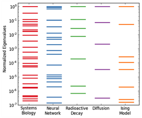
Figure 1: Sloppy eigenvalue spectra of multiparameter models from various fields Brown and Sethna (2003); Brown et al. (2004); Waterfall et al. (2006); Transtrum, Machta, and Sethna (2011); Machta et al. (2013). Eigenvalues of the FIM, indicating sensitivity to perturbations along orthogonal directions in parameter space, are roughly evenly spaced in log-space, extending over many orders of magnitude.

The degree of parameter indeterminacy in the simple sum-of-exponentials model has been seen in many complex models of real life systems for many of the same reasons. The FIMs for seventeen systems biology models have been shown to have the same characteristic eigenvalue structure Gutenkunst et al. (2007), and examples from other scientific domains abound Waterfall et al. (2006). In each case, observations measure a system’s collective behavior, and this means that when parameters have compensatory effects they cannot be individually identified.

The ubiquity of sloppiness would seem to limit the usefulness of complex parameterized models. If we cannot accurately know parameter values, how can a model be predictive? Surprisingly, predictions are possible without precise parameter knowledge. As long as the model predictions depend on the same stiff parameter combinations as the data, the predictions of the model will be constrained in spite of large numbers of poorly determined parameters.

The existence of a few stiff parameter combinations can be understood as a type of low effective dimensionality of the model. In section III we make this idea quantitative by considering a geometric interpretation of statistics. This leads naturally to a new method of model reduction that constructs low-dimensional approximations to high-dimensional models (section IV). These low-dimensional approximations are useful for revealing the emergent control mechanisms that govern the system’s behavior, i.e., extracting a simple emergent theory of the collective behavior from the larger, complex model.

Simple approximations to complex processes are common in physics (section V). The ubiquity of sloppiness suggests that similarly simple models can be constructed for other complex systems. Indeed, sloppiness has a number of profound implications for the unreasonable effectiveness of mathematics Wigner (1960) and the hierarchical structure of scientific theories Anderson et al. (1972). We discuss some of these consequences specifically for modeling biochemical networks in section VI. We discuss more generally the implications of sloppiness for mathematical modeling in section VII. We argue that sloppiness is the underlying reason why the universe (a complete description of which would be indescribably complex) is comprehensible.

II Mathematical Framework

In this section we use information theory to define key measures of sloppiness geometrically Amari and Nagaoka (2000). We first consider the special case of model selection for models fit to data by least squares. We then generalize to the case of arbitrary probabilistic models. The key insight is that the Fisher Information defines a Riemannian geometry on the space of possible models Amari and Nagaoka (2000). The geometric picture allows us to show (in section III) that this local sloppy structure in the metric is paralleled by a global hyper-ribbon structure of the entire space of possible models.

We begin with a simple case – a model ${\mathbf{y}}$ predicting data ${\mathbf{d}}$ at experimental conditions ${\mathbf{u}}$, with independent Gaussian errors; each of these are vectors whose length $M$ is given by the number of data points. Our model depends on $N$ parameters $\theta$. In general, an arbitrary model is a mathematical mapping from a parameter space into predictions, so interpreting a model as a manifold of dimension $N$ embedded in a data space ${\mathbb{R}}^{M}$ is natural; the parameters $\theta$ then become the coordinates for the manifold. If our error bars are independent and Gaussian all with the same width (say, $\sigma=1$), finding the best fit of model to data is a least squares data fitting problem, as we illustrate in Figure 2. In this case, we assume that each experimental data point, $d_{i}$, is generated from a parameterized model, $y(u_{i},\theta)$, plus random Gaussian noise, $\xi_{i}$:

$$d_{i}=y(u_{i},\theta)+\xi_{i}.$$ (2)

Since the noise is Gaussian,

$$P(\xi)\propto e^{-\xi^{2}/2},$$ (3)

maximizing the log likelihood is equivalent to minimizing the sum of squared residuals, sometimes referred to as the cost or $\chi^{2}$ function:

$$\chi^{2}(\theta)=\sum_{i}r_{i}^{2}=\sum_{i}\left(d_{i}-y(u_{i},\theta)\right)^{2}.$$ (4)

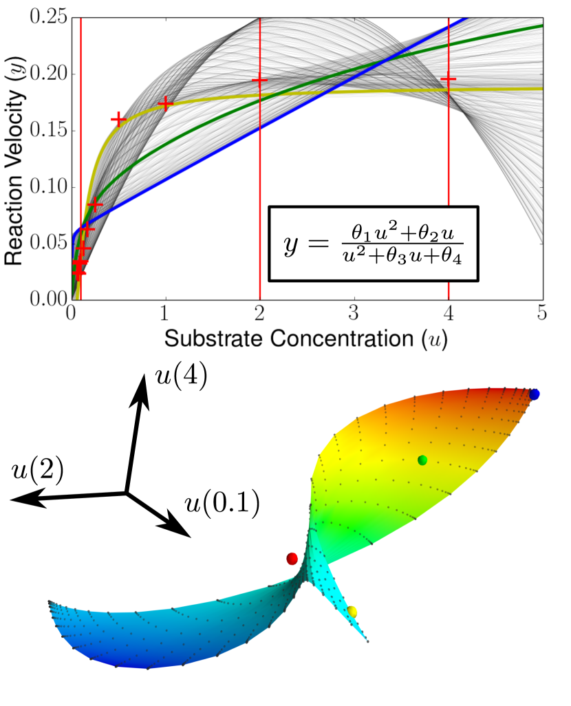
Figure 2: The Model Manifold A simple model Averick et al. (1992); Kowalik and Morrison (1968) of an enzyme-catalyzed reaction can be expressed as a rational function in substrate concentration ($u$) with four parameters ($\theta$) predicting the reaction velocity ($y$) (inset, top). By varying $\theta$ the model can predict a variety of behaviors $y$ as a function of $u$ (top). The model manifold is constructed by collecting all possible predictions of the model at specific values of $u$ (red vertical lines at $u=0.1,2.0,4.0$). To visualize the manifold, we take a two-dimensional cross section of the four dimensional manifold by choosing $\theta_{1}$ and $\theta_{2}$ to best fit the experimental data. Varying $\theta_{3}$ and $\theta_{4}$ then maps out a two-dimensional surface of possible values in three-dimensional data space (bottom). Each curve in the top figure corresponds to a point of the same color on the model manifold (bottom); the red crosses on top are data corresponding to the red dot below.

A sum of squares is reminiscent of a Euclidean distance. Fitting a model to data by least squares is therefore minimizing a distance in data space between the observed data and the model. Distance in data space measures the quality of a fit to experimental data (red point in Figure 2). Distance on the manifold is induced by, i.e., is the same as, the corresponding distance in data space and is measured using the metric tensor

$$g_{\mu\nu}=\sum_{i}\frac{\partial y(u_{i},\theta)}{\partial\theta^{\mu}}\frac{\partial y(u_{i},\theta)}{\partial\theta^{\nu}}=(J^{T}J)_{\mu\nu},$$ (5)

where $J_{i\mu}=\partial y(u_{i},\theta)/\partial\theta^{\mu}$ is the Jacobian matrix of partial derivatives. This metric tensor is precisely the Fisher Information Matrix (FIM) defined below, specialized to our least-squares problem. It is the least squares Hessian matrix of second derivatives of ${{}^{1}\mspace{-6.5mu}/\mspace{-4.5mu}_{2}}\chi^{2}$ from eqn 4, evaluated where the data point ${\mathbf{d}}$ is taken to be perfectly predicted by ${\mathbf{y}}({\mbox{\boldmath$\theta$}})$. On the manifold, distance is a measure of identifiability – how difficult it would be to distinguish nearby points on the manifold (i.e., alternate models) through their predictions.

We can generalize from this least-squares fitting problem to encompass other models (like the Ising model) where the predictions are for entire probability distributions. For the purpose of modeling, the output of our model is a probability distribution for $x$, the outcome of an experiment. A parameterized space of models is thus defined by $P(x|\theta)$. To define a geometry on this space we must define a measure of how distinct two points $\theta_{1}$ and $\theta_{2}$ in parameter space are, based on their predictions. Imagine getting a sequence of assumed independent data $x_{1},x_{2},...$ with the task of inferring the model which produced them. The likelihood that model $\theta_{1}$ would have produced this data is given by

$$P(x_{1},x_{2},...|\theta)=\prod_{i}P(x_{i}|\theta)=\exp{\left(\sum_{i}\log{P(x_{i}|\theta)}\right)}.$$ (6)

In maximum likelihood estimation our goal is simply to find the parameter set $\theta$ which maximizes this likelihood. It is useful to talk about $\log{P(x|\theta)}$, the log-likelihood, as this is the unique measure which is additive for independent data points. The familiar Shannon entropy of a model’s predictions $x$ is given by minus the expectation value of the log-likelihood:

$$S(\theta)=-\sum_{x}P(x|\theta)\log{P(x|\theta)}.$$ (7)

We can also define an analogous quantity that measures the likelihood that model $\theta_{2}$ would produce typical data from $\theta_{1}$:

$$\sum_{x}P(x|\theta_{1})\log{P(x|\theta_{2})}.$$ (8)

The Kullback-Leibler divergence between $\theta_{1}$ and $\theta_{2}$ measures how much more likely $\theta_{1}$ is to produce typical data from $\theta_{1}$ than $\theta_{2}$ would be:

$$D_{\mathrm{KL}}(\theta_{1}||\theta_{2})=\sum_{x}P(x|\theta_{1})\big{(}\log{P(x|\theta_{1})}-\log{P(x|\theta_{2})}\big{)}.$$ (9)

Thus $D_{\mathrm{KL}}$ is an intrinsic measure of how difficult distinguishing these two models will be from their data.

The KL divergence does not satisfy the mathematical requirements of a distance measure. It is asymmetric, and does not satisfy even a weak triangle inequality: In some cases $D_{\mathrm{KL}}(\theta_{1}||\theta_{3})>D_{\mathrm{KL}}(\theta_{1}||\theta_{2})+D_{\mathrm{KL}}(\theta_{2}||\theta_{3})$. However, for models whose parameters $\theta$ and $\theta+\delta\theta$ are quite close to one another, the leading terms are symmetric and can be written as:

$$D_{\mathrm{KL}}(\theta||\theta+\delta\theta)=g_{\mu\nu}\delta\theta^{\mu}\delta\theta^{\nu}+\mathcal{O}\delta\theta^{3}$$ (10)

where $g_{\mu\nu}$ is the Fisher Information Matrix (FIM), which can be written:

$$g_{\mu\nu}(P_{\theta})=-\sum_{x}P_{\theta}(x)\frac{\partial}{\partial\theta^{\mu}}\frac{\partial}{\partial\theta^{\nu}}\log P_{\theta}(x).$$ (11)

The FIM has all the properties of a metric tensor. It is symmetric and positive semi-definite (because no model can on average be better described by a different model) and it transforms properly under a coordinate reparameterization of $\theta$. Information Geometry Beale (1960); Bates and Watts (1980); Amari (1985); Amari et al. (1987); Murray and Rice (1993); Amari and Nagaoka (2007); Transtrum, Machta, and Sethna (2010, 2011) is the study of the properties of the model manifold defined by this metric. In particular, it defines a space of models in a way that does not depend on the labels given to the parameters, which are presumably arbitrary; should one measure rate constants in seconds or hours, and more problematically, should one label these constants as rates, or time constants? Information Geometry makes clear that some aspects of a parameterized model can be defined in ways that are invariant to these arbitrary choices.

III Why Sloppiness? Information Geometry

Sloppy models can be identified by the characteristic eigenvalue spectrum of the FIM. We interpret the existence of many small eigenvalues in the FIM to be representative of a complex model with a low effective dimensionality. Many combinations of parameters have minimal effect on the behavior of the model, while the key features of model behavior are controlled by a relatively small number of stiff parameter combinations. In a sense, then, there really is a simpler ‘theory’ embedded in the multiparameter ‘model’.

In this section we make the notion of low effective dimensionality explicit. We will see that although this interpretation of sloppy models turns out to be correct, the eigenvalues of the FIM are not sufficient to make this conclusion. Instead, we use the geometric interpretation of modeling introduced in section II that allows us to quantify important features of the model in a global and parameterization independent way. The effort to develop this formalism will pay further dividends when we consider model reduction in section IV.

To understand the limitations of interpreting the eigenvalues of the FIM, we return to the question of model reparameterization. Something as trivial as changing the units of a rate constant from Hz to kHz changes the corresponding row and column of the FIM by a factor of 1000, in turn changing the eigenvalues. Of course, none of the model predictions are altered by such a change since a correcting factor of 1000 will be introduced throughout the model. More generally, the FIM can be transformed into any positive definite matrix by a simple linear transformation of parameters while model predictions are always invariant to such a reparameterization.

Although the FIM eigenvalues are not invariant to reparameterization, we can use information geometry to search for a parameterization independent measure of sloppiness. With the definitions of section II, computational differential geometry can be used to explore the a wide variety of model manifolds in a parameter independent way. A review of these methods is beyond the scope of this paper, and we refer the interested reader to references Transtrum, Machta, and Sethna (2010, 2011) or any standard text on differential geometry Spivak (1979); Ivancevic (2007).

The key geometric feature of the model manifolds of nonlinear sloppy systems is that they have boundaries. Many parameters and parameter combinations can be taken to extreme values (zero or infinity) without leading to infinite predictions. These boundaries can be explored by numerically constructing manifold geodesics: analogs of straight lines on curved surfaces. The arc lengths of geodesics are a measure of the width of the model manifold in each direction. Measuring these arc lengths for a sloppy model shows that the widths of sloppy model manifolds are exponentially distributed, reminiscent of the exponential distribution of FIM eigenvalues. Indeed, when we use dimensionless model parameters (e. g. log-parameters), the square roots of the FIM eigenvalues are a reliable approximation to the widths of the manifold in the corresponding eigendirections Transtrum, Machta, and Sethna (2010, 2011).

The exponential distribution of manifold widths has been described as a hyperribbon (Fig. 3). A three-dimensional ribbon has a long dimension, a broad dimension, and a very thin dimension. The observed hierarchy of exponentially decreasing manifold widths are a high-dimensional generalization of this structure. We will explore the nature of these boundaries in more detail when we discuss model reduction in section IV.

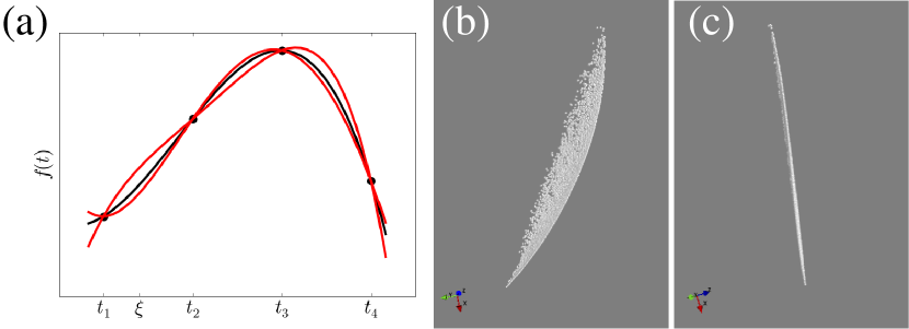
Figure 3: Hyperribbon. (a) Given a multiparameter model for one-dimensional data $f(t)$ at different times $t$, the model manifold has a different dimension for every time $t$. Specifying a data point $f(t_{n})$ thus gives a cross-section of the model manifold, and also reduces the uncertainty in the values of neighboring points – hence giving the cross-section a narrower width – a hyperribbon. Interpolation theory Transtrum, Machta, and Sethna (2010, 2011) can be used to quantify this qualitative argument. (Figure from fig. 5 of Transtrum, Machta, and Sethna (2011).) (b,c) Two views of a hyperribbon cross section of a model manifold. The model is decaying exponentials fit to radioactive decay data Waterfall et al. (2006). Notice the ribbon-like structure of this three-dimensional projection: long, narrow, and very thin.

The observed hierarchy of widths can be demonstrated analytically for the case of a single independent variable (such as time or substrate concentration in Figure 2) by appealing to theorems for the convergence of interpolating functions (Fig. 3(a)). Consider removing a few degrees of freedom from a time series by fixing the output of the model at a few time points. The resulting model manifold corresponds to a cross-section of the original. Next, consider how much the predictions at intermediate time points can be made to vary as the remaining parameters are scanned. As more and more predictions are fixed (i.e., considering higher-dimensional cross sections of the model manifold), we intuitively predict that the behavior of the model at intermediate time points will become more constrained. Interpolation theorems make this intuition formal; presuming smoothness or analyticity of the predictions as a function of time, one can demonstrate an exponential hierarchy of widths consistent with the hyperribbon structure observed empirically Transtrum, Machta, and Sethna (2010, 2011).

The exponential hierarchy of manifold widths makes explicit the notion of a low effective dimensionality in the model that was hinted at by the eigenvalues of the FIM. It also helps illustrate how models can be predictive without parameters being tightly constrained. Only those parameter combinations that are required to fit the key features of the data need to be estimated accurately. The remaining parameter combinations (controlling for example the high-frequency behavior in our time series example) are unnecessary. In short, the model essentially functions as an interpolation scheme among observed data points. Models are predictive with unconstrained parameters when the predictions interpolate among observed data.

Understanding models as generalized interpolation schemes makes additional predictions about the generic structure of sloppy model manifolds. Not only is there an exponential distribution of widths, there is also an exponential distribution of extrinsic curvatures. Furthermore, these curvatures are relatively small in relation to the widths, making the model manifold surprisingly flat. Most of the nonlinearity of the model’s parameters take the form of ‘parameter effects curvature’ Bates and Watts (1980, 1981); Bates, Hamilton, and Watts (1983); Bates and Watts (1988), (equivalent to the connection coefficients Transtrum, Machta, and Sethna (2011)). The small extrinsic curvature of many models was a mystery first noted in the early 1980s Bates and Watts (1980) that is explained by interpolation arguments.

IV Model Reduction

In this section, we leverage the power of the information geometry formalism to answer the question: how can a simple effective model be constructed from a (more-or-less) complete but sloppy representation of a physical system? Our goal is to construct a physically meaningful representation that reveals the simple ‘theory’ that is hidden in the model.

The model reduction problem has a long history, and it would be impossible in this review to even approach a comprehensive survey of literature on the subject. Several standard methods have emerged that have proven effective in appropriate contexts. Examples include clustering components into modules Wei and Kuo (1969); Liao and Lightfoot (1988); Huang et al. (2005), mean field theory, various limiting approximations (e.g., continuum, thermodynamic, or singular limits), and the renormalization group Goldenfeld (1992); Zinn-Justin (2007). Considerable effort has been devoted by the control and engineering communities to approximate large-scale dynamical systems Saksena, O’reilly, and Kokotovic (1984); Kokotovic, Khali, and O’Reilly (1999); Naidu (2002); Antoulas (2005); Lee and Othmer (2010), leading to the method of balanced truncation Moore (1981); Dullerud and Paganini (2000); Gugercin and Antoulas (2004), including several structure preserving variations Zhou, D’Souza, and Cloutier (1995); Li and Paganini (2005); Sandberg and Murray (2009) and generalizations to nonlinear cases Scherpen (1993); Lall, Marsden, and Glavaški (2002); Krener (2008). Methods for inferring minimal dynamical models in cases for which the underlying structure is not known are also beginning to be developed Daniels and Nemenman (2014, 2015).

Unfortunately, many automatic methods produce ‘black box’ approximations. For most scenarios of practical importance, a reduced representation alone has limited utility since attempts to engineer or control the system typically operate on the microscopic level. For example, mutations operate on individual genes and drugs target specific proteins. A method that explicitly reveals how microscopic components are ‘compressed’ into a few effective degrees of freedom would be very useful. On the other hand, methods that do explicitly connect microscopic components to macroscopic behaviors have limited scope since they often exploit special properties of the model’s functional form, such as symmetries. Consider, for example, the renormalization group, which operates on field theories with a scale invariance or conformal symmetry. Simplifying modular network systems, such as biochemical networks, is particularly challenging due to inhomogeneity and lack of symmetries.

The Manifold Boundary Approximation Method (MBAM) Transtrum and Qiu (2014) is an approach to model approximation whose goal is to alleviate these challenges. As the name implies, the basic idea is to approximate a high-dimensional, but thin model manifold by its boundary. The procedure can be summarized as a four step algorithm. First, the least sensitive parameter combination is identified from an eigenvalue decomposition of the FIM. Second, a geodesic on the model manifold is constructed numerically to identify the boundary. Third, having found the edge of the model manifold, the corresponding model is identified as an approximation to the original model. Fourth, the parameter values for this approximate model are calibrated by fitting the approximate model to the behavior of the original model.

The result of this procedure is an approximate model that has one less parameter and that is marginally less sloppy than the original. Iterating the MBAM algorithm therefore produces a series of models of decreasing complexity that explicitly connect the microscopic components to the macroscopic behavior. These models correspond to hyper-corners of the original model manifold. The method requires only that the model manifold have a hierarchy of boundaries while making no assumptions about the mathematical form of the model or underlying physics of the system. As such, MBAM is a very general approximation scheme.

The key component that enables MBAM are the edges of the model manifold. The existence of these edges was first noted in the context of data fitting Transtrum, Machta, and Sethna (2010) and MCMC sampling of Bayesian posterior distributions Gutenkunst (2007). It was noted that algorithms would often ‘evaporate’ parameters, i.e., allow them to drift to extreme, usually infinite, values. These extreme parameter values correspond to limiting behaviors in the model, i.e., manifold boundaries.

‘Evaporated parameters’ are especially problematic for numerical algorithms. Numerical methods often push parameters to the edge of the manifold and then become lost in parameter space. Consider the case of MCMC sampling of a Bayesian posterior. If a parameter drifts to infinity, there is an infinite amount of entropy associated with that region of parameter space and the sampling will never converge. Furthermore, the model behavior of such a region will always dominate the posterior distribution Gutenkunst (2007).

For data fitting algorithms, methods such as Levenberg-Marquardt operate by fitting the key features of the data first (i.e., the stiffest directions), followed by successive refining approximations (i.e., progressively more sloppy components). While fitting the initial key features, algorithms often evaporate those parameters associated with less prominent features of the data. The algorithm is then unable bring the parameters away from infinity in order to further refine the fit Transtrum, Machta, and Sethna (2010).

Although problematic for numerical algorithms, manifold edges are useful for both approximating (ala MBAM) and interpreting complex models. To illustrate, we consider an EGFR signaling modelBrown and Sethna (2003). Figure 4 illustrates components of one eigenparameter, corresponding in this case to the smallest eigenvalue of the FIM. Notice that the eigenparameters do not align with bare parameters of the model, but typically involve an unintuitive combination of bare parameters. However, by following a geodesic along the model manifold to the manifold edge (step 2 of the MBAM algorithm), these complex combinations slowly rotate to reveal relatively simple, interpretable combinations that correspond to a limiting approximation of the model. For example, the EGFR model in reference Brown and Sethna (2003) consists of a network of Michaelis-Menten reactions. The boundary revealed Transtrum and Qiu (2014) in Figure 4 corresponds to the limit of a reaction rate and a Michaelis-Menten constant becoming infinite while their ratio is finite:

$$\frac{d}{dt}[A] = \frac{k[A][B]}{K_{M}+[A]}+\dots$$ (12)

$$\rightarrow \left(\frac{k}{K_{M}}\right)[A][B]+\dots,$$ (13)

where $[A]$ and $[B]$ are concentrations of two enzymes in the model and the ratio $k/K_{M}$ is the renormalized parameter in the approximate model.

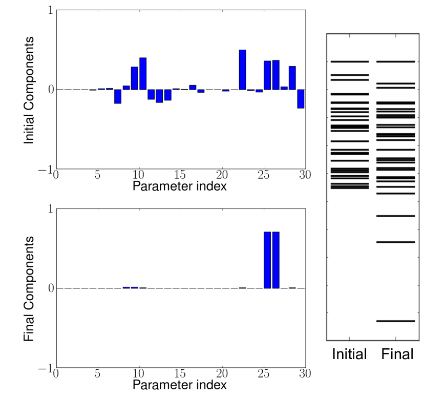
Figure 4: Identifying the boundary limit Transtrum and Qiu (2014). The components of the smallest eigenvector of the FIM is often a complicated combination of bare parameters that is difficult to either interpret or remove from the model (top left). By following a geodesic to the manifold boundary, the combination rotates to reveal a limiting behavior (bottom left); here two parameters (a reaction rate and a Michaelis-Menten constant) become infinite. The limiting behavior is revealed when the smallest eigenvalue has become separated from the other eigenvalues (right).

Because the manifold edges correspond to models that are simple approximations of the original, the MBAM can be used to iteratively construct simple representations of otherwise complex processes. By combining several limiting approximations, simple insights into the system behavior emerge that were obfuscated by the original model’s complexity. Figure 5 compares network diagrams for the original and approximate EGFR models. The original consists of 29 differential equations and 48 parameters, while the approximate consists of 6 differential equations and 12 parameters and is notably not sloppy.

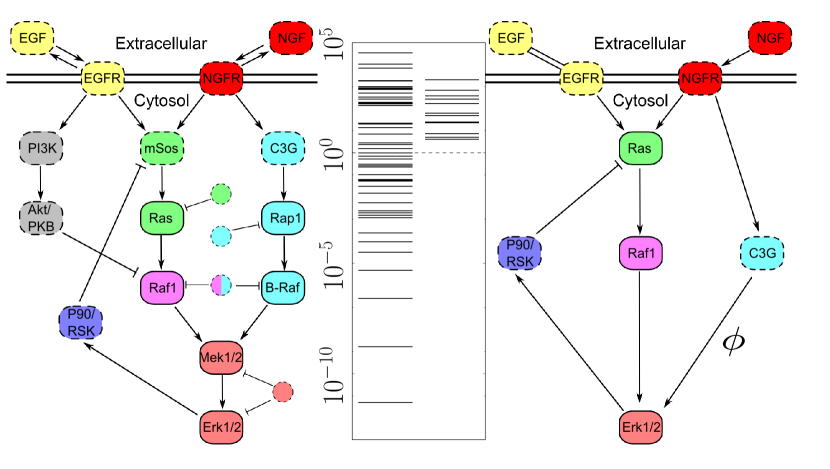
Figure 5: Original Brown and Sethna (2003) and reduced Transtrum and Qiu (2014) EGFR models. The interactions of the EGFR signaling pathway Brown and Sethna (2003); Brown et al. (2004) are summarized in the leftmost network. Solid circles are chemical species for which the experimental data was available to fit. Manifold boundaries reduce the model to a form (right) capable of fitting the same data and making the same predictions as in the original references Brown and Sethna (2003); Brown et al. (2004). The FIM eigenvalues (center) indicate that the simplified model has removed the irrelevant parameters identified as eigenvalues less than $1$ (dotted line) while retaining the original model’s predictive power.

Because the MBAM process explicitly connects models through a series of limiting approximations, the parameters of the reduced model can be identified with (nonlinear) combinations of parameters in the original model. For example, one of the twelve variables in the reduced model of Fig. 5 is written as an explicit combination of seven ‘bare’ parameters of the original model:

$$\phi=\frac{(\mathrm{k_{Rap1ToBRaf}})(\mathrm{K_{mdBRaf}})(\mathrm{k_{pBRaf}})(\mathrm{K_{mdMek}})}{(\mathrm{k_{dBRaf}})(\mathrm{K_{mRap1ToBRaf}})(\mathrm{k_{dMek}})}.$$ (14)

Expressions such as this explicitly identify which combinations of microscopic parameters act as emergent control knobs for the system.

MBAM naturally includes many other approximation methods as special cases Transtrum and Qiu (2014). By an appropriate choice of parameterization, it is both a natural language for model reduction and a systematic method that in practice can be mostly automated.

The MBAM is a semi-global approximation method. Manifold boundaries are a non-local feature of the model. However, MBAM only explores the region of the manifold in the vicinity of a single hyper-corner. More generally, it is possible to identify all of the edges of a particular model (and by extension, all possible simplified models). This analysis is known information topology Transtrum, Hart, and Qiu (2014).

V Emergence in Physics as sloppiness

Unlike in systems biology, physics is dominated by effective models and theories whose forms are often deduced long before a microscopic theory is available. This is in large part due to the great success of continuum limit arguments and Renormalization Group (RG) procedures in justifying the expectation and deriving the form of simple emergent theories. These methods show that many different multi-parameter microscopic theories typically collapse onto one coarse-grained model, with the complex microscopics being summarized into just a few ‘relevant’ coarse-grained parameters. This explains why an effective theory, or an oversimplified ‘cartoon’ microscopic theory, can often make quantitatively correct predictions. Thus, while three dimensional liquids have enormous microscopic diversity, in a certain regime (lengths and times large compared to molecules and their vibration periods), their behavior is determined entirely by their viscosity and density. Although two different liquids can be microscopically completely different, their effective behavior is determined only by the projection of their microscopic details onto these two control parameters. This parameter space compression underlies the success of renormalizable and continuum limit models.

This connection has been made explicit, by examining the FIM for typical microscopic models in physics Machta et al. (2013). A microscopic hopping model for the continuum diffusion equation quickly develops ‘stiff’ directions corresponding to the parameters of the continuum theory – the total number of particles, net mean velocity, and diffusion constant. As time evolves, all other microscopic parameter combinations become increasingly sloppy – irrelevant for prediction of long-time behavior. Similarly, a microscopic long-range Ising model for ferromagnetism, when observed on long length scales, develops stiff directions along precisely those parameter combinations deemed ‘relevant’ under the renormalization group.

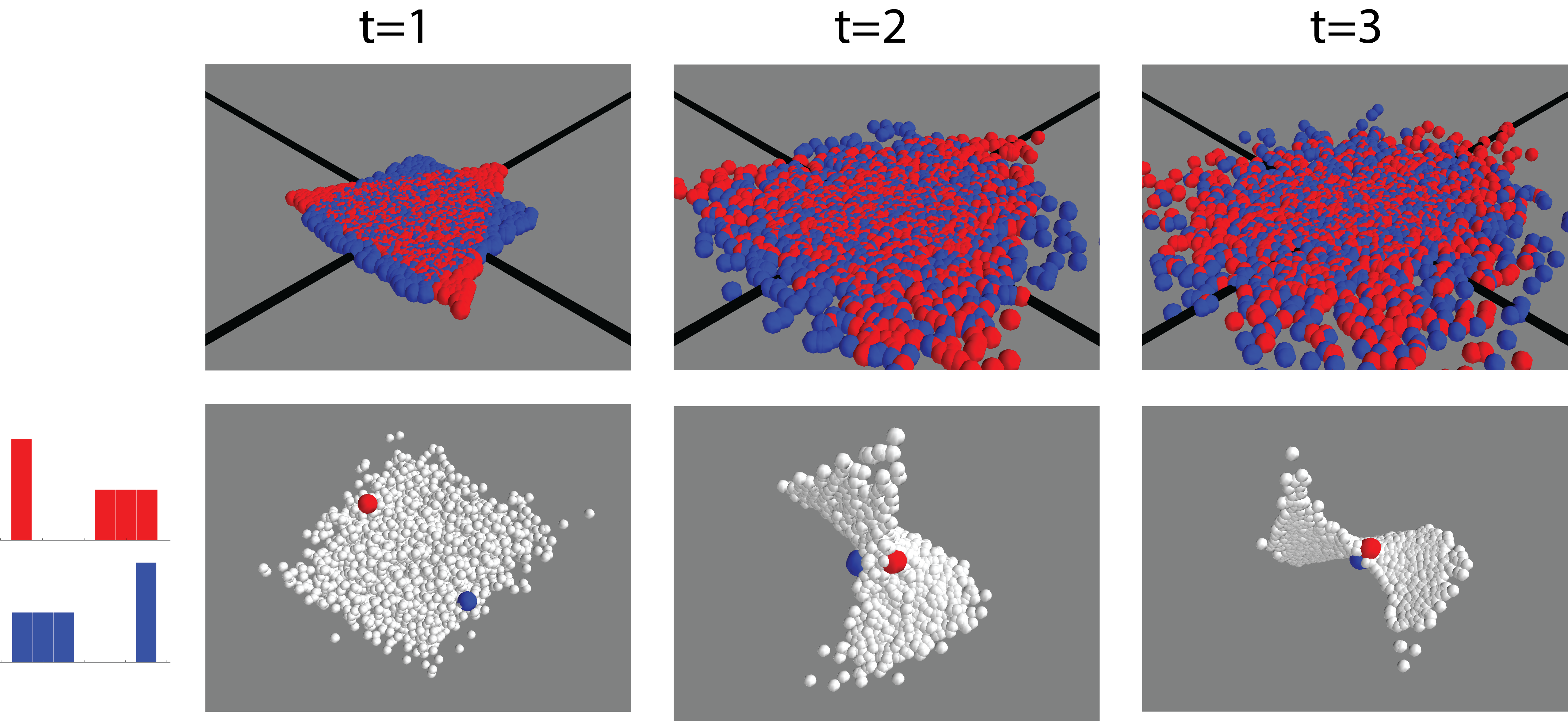
Figure 6: Microscopic Motion becomes Diffusive. Top: Simulated particles undergo stochastic motion in discrete time. Red particles hop according to a triangular kernel, while blue particles hop according to a square kernel. After a single time step, the particles have very different distributions in space, and neither resemble the distribution predicted by the diffusion equation. However, as time evolves, most of the information about this kernel is lost. Only the particles’ diffusion tensor and average drift enter into a continuum description. For the particles shown, the drift is 0, and their respective diffusion tensors are matched, so that the resulting distributions become quantifiably indistinguishable as time proceeds. The compression of microscopic details mirrors the compression of molecular level detail in the emergence of diffusion as a continuum limit of motion in real fluids. Bottom: We consider the model manifold of a one dimensional lattice version of this diffusion example. As with the triangle and square, the red and blue kernels shown on the left have drift 0, and identical second moments, though higher moments and the distribution in general are very different. The remaining white points making up the manifold are taken from a uniform distribution in parameter space describing the probability of hopping to one of six nearest neighbors in a given time step, as in Ref. Machta et al. (2013). Here we plot a three dimensional projection of the model manifold taken from measurements of particle distributions at different time points. After a single time step, this three dimensional projection from data space shows a ‘hyper-blob’, with changes in parameters leading to a large diversity of observable behaviors. In particular, the red and blue points are not close to each other even though their drifts are both 0 and their diffusion constants are matched; as with the square and triangle, their distributions are easily distinguishable after a single time step. However, after several stochastic steps, the model manifold takes on a hyperribbon structure. Models for which all effective parameters are matched, like the red and blue kernels highlighted, rapidly move close to each other. At late times, any model sufficiently flexible to capture the two remaining extended directions is adequate to describe effective behavior, explaining the ubiquity and success of the continuum diffusion equation.

Consider a model of stochastic motion as a stand-in for a molecular level description of particles moving through a possibly complicated fluid. Such a fluid’s properties depend on many parameters such as the bond angle of the molecules which make it up, all of which enter into the probability distribution for motion within the fluid, which can presumably be microscopically complex. However, the law of large numbers says that as many of these random steps are added together, the long-time movement of particles will lead to them being distributed in space according to a Gaussian. As this happens, diverse microscopic details must become compressed into the two parameters of a Gaussian distribution- its mean and width. As a concrete example, in the top of Figure 6, two very different microscopic motions are considered. In each time step, red particles take a random step from a triangular distribution, while blue particles step according to a square distribution. While these motions lead to very different distributions after a single time step, as time proceeds they become indistinguishable precisely because their first and second moments are matched.

This indistinguishability can be quantified by considering the model manifold of possible microscopic models of stochastic motion, again paralleling real fluids that can be microscopically diverse. When probed at the intrinsic time and length scales of these fluids, we should make few assumptions about the type of motion we expect; in particular, we should allow for behaviors much more complicated than diffusion, by analogy with square and triangle described in two dimensions above. Following Ref. Machta et al. (2013), we consider a one dimensional ‘molecular level’ model for stochastic motion, in which parameters describe the rates at which a particle hops to one of its close-by neighbors. After a single time step, the corresponding model manifold is a ‘hyper-blob’ (fig. 6, bottom) and two particular models, marked in red and blue, are distinguishable; they are not nearby on the model manifold. The prediction space of a model is truly multidimensional in this regime- it cannot be described by the two parameter diffusion equation. In this ‘ballistic’ regime, motion is not described by the diffusion equation, and is presumably not just different, but genuinely more complicated. However, as time proceeds, the model manifold contracts onto a hyper-ribbon, in which just two parameter combinations distinguish behavior. In this regime, all points lie close to the two dimensional manifold predicted by the diffusion equation, and the red and blue points have become indistinguishable; they are now in close proximity on the manifold.

Using information geometry, approximations analogous to continuum limits or the renormalization group can be found and used to construct similarly simple theories in fields for which effective theories have historically been difficult to construct or justify.

VI Ramifications of Sloppiness in Biochemical Modeling

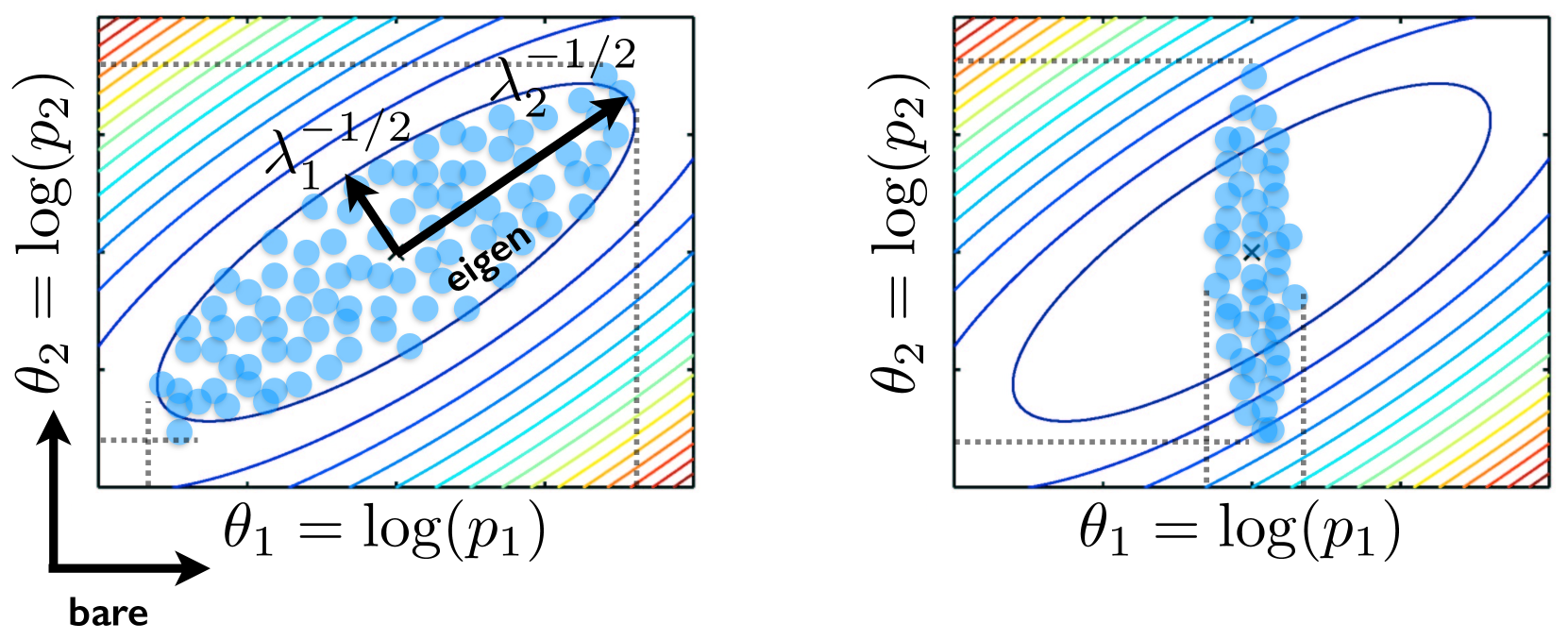
Figure 7: Sloppiness in Parameter Space. Left: A schematic of a typical Sloppy Model ensemble, pictured in two dimensions for clarity. The underlying cost surface (with constant cost contours illustrated as ellipses) is generated by the fit to data. Eigenvectors of the FIM correspond to principal axes of the ellipse, with widths of the ellipse inversely proportional to the square roots of the corresponding eigenvalues $\lambda_{i}$. Points inside the ellipse each represent a set of parameters that fits the data within a given tolerance (in practice often created using a Monte Carlo approach), forming an ensemble representing uncertainty about the true values of parameters. Sloppiness can result in good fits to data despite enormous uncertainties in ‘bare’ $\theta$ parameters (dotted lines intersecting the axes). Right: Careful measurements of individual parameters (like $\theta_{1}$) can shrink uncertainty, but if even a single parameter remains unknown (like $\theta_{2}$), large predictive uncertainty can still result.

In previous sections, we have emphasized picturing the model manifold in data space, as in Figure 2; here, thin, sloppy dimensions of the hyperribbon correspond to behavior that is minimally dependent on parameters. The dual picture in parameter space, sketched in Figure 7, is one in which the set of parameters that sufficiently well fit some given data is stretched to extend far along sloppy dimensions. This picture is important to understanding implications for biochemical modeling with regard to parameter uncertainty.

For instance, using the full EGFR signal transduction network (left side of Figure 5), we may wish to make a prediction about an unmeasured experimental condition, e.g. the time-course of ERK activity upon EGF stimulation. In general, if there are large uncertainties about the model’s parameters, we expect our uncertainty about this time-course to also be large.

Indeed this is the case if we neglect effects of compensation among parameters and assume that uncertainties in different parameters are uncorrelated. If we view the problem of uncertainties in model predictions as coming from a lack of precision measurements of individual parameters, we may try to carefully and independently measure each parameter. This can work if such measurements are feasible, but can fail if even one relevant parameter remains unknown: as in the right plot of Figure 7, a large uncertainty along the direction of a single parameter corresponds to large changes in system-level behavior, leading to large predictive uncertainties Gutenkunst et al. (2007).

Contrasting with this approach, we can instead constrain the model parameters with system-level measurements that are similar to the types of measurements we wish to predict. Due to the phenomenon of sloppiness, we expect that this approach will produce a subspace of acceptable parameters that will include large uncertainties in individual parameter values (left plot of Figure 7). Again, this arises because two parameters that change the output in a correlated way can consequently be simultaneously varied without changing the model output. It is often true that variance of system-level measurements over the large sloppy parameter subspace is as small as would require extremely precise measurements if parameters were measured independently. Predictions of interest can be made without precisely knowing any single parameter.

Thus, in the sense that estimating parameters entails discovering their precise values, in sloppy models parameter estimation becomes useless. This does not mean that anything goes; the region of acceptable parameters may be small compared to prior knowledge about their values. Yet it does validate a common approach to modeling such systems, in which educated guesses are made for most parameters, and a remaining handful are fit to the data. In the common situation in which there are a small number $m$ of important ‘stiff’ directions, with remaining sloppy directions extending to cover the full range of feasible parameters, fitting $m$ parameters will be enough to locate the sloppy subspace. (And if using a maximum likelihood approach, this is in fact statistically preferred to fitting all parameters, in order to avoid overfitting.) Unfortunately, it is hard to know $m$ ahead of time, in general requiring a sampling scheme like MCMC or a geodesic-following algorithm Transtrum, Machta, and Sethna (2010, 2011) to ascertain the global structure of the sloppy subspace.

The problem of parameter estimation has been central to the field of systems biology for many years. The extremely large uncertainties in parameter estimates led to the suggestion that accurate parameter estimates might not be possible Gutenkunst et al. (2007). However, advances in experimental design have suggested that such estimates might be feasible after all Apgar et al. (2010); Vilela et al. (2009); Erguler and Stumpf (2011); Transtrum and Qiu (2012), although requiring considerable experimental effort Chachra, Transtrum, and Sethna (2011). The perspective provided by sloppy model analysis provides at least two alternatives to this method of operation.

First, in spite of the large number of parameters, complex biological systems typically exhibit simple behavior that requires only a few parameters to describe, analogous to how the diffusion equation can describe microscopically diverse processes. Attempting to accurately infer all of the parameters in a complex biological model Lee et al. (2008) is analogous to learning all of the mechanical and electrical properties of water molecules in order to accurately predict a diffusion constant. It would involve considerable effort (measuring all the microscopic parameters accurately Gutenkunst et al. (2007)), while the diffusion constant can be easily measured using collective experiments, and used to determine the result of any other collective experiment.

Second, in many biological systems, there is considerable uncertainty about the microscopic structure of the system. Sloppiness suggests that an effective model that is microscopically inaccurate may still be insightful and predictive in spite of getting many specific details wrong. For example a hopping model for thermal conductivity would be ‘wrong’ even though it gives the right thermal diffusion equation. ‘Wrong’ models can provide key insights into the system level behavior because they share important features with the true system. In such a scenario, it is the flexibility provided by large uncertainties in the parameters that allows the model to be useful. Any attempt to infer all the microscopic parameters would break the model, preventing it from being able to fit the data.

Indeed, it is difficult to envision a completely microscopic model in systems biology. Any model will have rates and binding affinities that will be altered by the surrounding complex stew of proteins, ions, lipids, and cellular substructures. Is the well-known dependence of a reaction rate on salt concentration (described by an effective Gibbs free energy tracing over the ionic degrees of freedom) qualitatively different from the dependence of an effective reaction rate on cross-talk, regulatory mechanisms, or even parallel or competing pathways not incorporated into the model? We are reminded of quantum field theories, where the properties (say) of the electron known to quantum chemistry are renormalized by electron-hole reactions in the surrounding vacuum which are ignored and ignorable at low energies. Insofar as a model provides both insight and correct predictions within its realm of validity, the fact that its parameters have effective, renormalized values incorporating missing microscopic mechanisms should be expected, not disparaged.

VII More general consequences of sloppiness

The hyperribbon structures implied by interpolation theory and information geometry in section III have profound implications. Complex scientific models have predictions that vary in far fewer ways than their complexity would indicate. Multiparameter models have behavior that largely depend upon only a few combinations of microscopic parameters. The high-dimensional results of a system with a large number of control parameters will be well encompassed by a rather flat, low-dimensional manifold of behavior. In this section, we shall speculate about these larger issues, and how they may explain the success of our efforts to organize and understand our environment.

Efficacy of Principal Component Analysis. Principal component analysis, or PCA, has long been an effective tool for data analysis. Given a high-dimensional data set, such as the changes of mRNA levels for thousands of genes under several experimental conditions Ringner (2008), PCA provides a reduced-dimensional description which often retains most of the variation in the original data set in a few linear components. Arranging the data into a matrix $R_{jn}+c_{j}$ of experiments $n$ and data points $j$ centered at $c_{j}$, PCA uses the singular value decomposition (SVD)

$$R =\sum_{k}\sigma_{k}\hat{{\mathbf{u}}}^{(k)}\otimes\hat{{\mathbf{v}}}^{(k)}$$ (15)

$$R_{jn} =\sum_{k}\sigma_{k}\hat{u}^{(k)}_{j}\hat{v}^{(k)}_{n}$$ (16)

to write $R$ as the sum of outer products of orthonormal vectors $\hat{\mathbf{u}}^{(k)}$ in data space and $\hat{\mathbf{v}}^{(k)}$ in the space of experiments. Here $\sigma_{1}\geq\sigma_{2}\geq...\geq 0$ are nonnegative ‘strengths’ of the different components $k$. These singular values can be viewed as a generalization of eigenvalues for non-square, non-symmetric matrices. The $\hat{{\mathbf{u}}}^{(k)}$ for small $k$ describe the ‘long axes’ of the data, viewed as a cloud of points ${\mathbf{R}}_{n}$ in data space; $\sigma_{k}$ is the RMS extent of the cloud in direction $\hat{{\mathbf{u}}}^{(k)}$. The utility of PCA stems from the fact that in many circumstances only a few components $k$ are needed to provide an accurate reconstruction of the original data. Just as our sloppy eigenvalues converge geometrically to zero, the singular values $\sigma_{k}$ often rapidly vanish. It is straightforward to show that the truncated SVD keeping only the first, largest $K$ components is an optimal approximation to the data, with total least square error bounded by $\sum_{K+1}\sigma_{k}^{2}$. These largest singular components often have physical or biological interpretations – sometimes mundane but useful (which machine was used to take the data), sometimes scientifically central.

Why does Nature often demand so few components to describe large dimensional data sets? Sloppiness provides a natural explanation. If the data results from (say) a biological system whose behavior is described by a sloppy model ${\mathbf{y}}({\mbox{\boldmath$\theta$}})$, and if the different experiments are sampling different parameter sets ${\mbox{\boldmath$\theta$}}_{n}$, then the data will be points $R_{jn}+c_{j}=y_{j}({\mbox{\boldmath$\theta$}}_{n})$ on the model manifold. Insofar as the model manifold has the hyperribbon structure we predict, it has only a few long axes (corresponding to stiff directions) and it is extrinsically very flat along these axes (Transtrum, Machta, and Sethna, 2011, Fig. 18). Here each $y_{j}-c_{j}$, being a difference between a data point and the center of the data, will be nearly a linear sum of a small number $K$ of long directions of the model manifold, and the RMS spread along this $k^{\mathrm{th}}$ direction will be bounded by the width of the model manifold in that direction, plus a small correction for the curvature. As any cloud of experimental points must be bounded by the model manifold, the high singular values will be bounded by the hierarchy of widths of the hyperribbon. Hence our arguments for the hyperribbon structure of the model manifold in multiparameter models provide a fundamental explanation for the success of PCA for these systems.

Efficacy of Levenberg-Marquardt; improved algorithms.

The Levenberg-Marquardt algorithm Levenberg (1944); Marquardt (1963); Press et al. (2007) is one of the standard algorithms for least squares minimization. Its broad utility can be explained through the lens of sloppy models and geometric insights lead to natural improvements. Minimizing a linear approximation to a nonlinear model with a constraint on the step size

$$\min_{\delta\theta}\left|y(\theta_{0})+J\delta\theta-y_{0}\right|^{2},\ \ \ \left|\delta\theta\right|\leq\Delta$$ (17)

leads to the iterative algorithm

$$\delta\theta=-\left(J^{T}J+\lambda\right)^{-1}J^{T}\left(y(\theta_{0})-y_{0}\right),$$ (18)

where $\lambda$ is a Lagrange multiplier. The FIM ($J^{T}J$) for a typical sloppy model is extremely ill-conditioned. However, the dampened scaling matrix $J^{T}J+\lambda$ will have no eigenvalues smaller than $\lambda$. By tuning $\lambda$, the algorithm is able to explicitly control the effects of sloppiness. Furthermore, since the eigenvalues of $J^{T}J$ are roughly log-linear, $\lambda$ need not be finely tuned to be effective. By slowly decreasing $\lambda$, the algorithm fits the key features of the data first (i.e., the stiffest directions), followed by successive refining approximations (i.e., progressively more sloppy components). The algorithm may still converge slowly as it navigates the extremely narrow canyons of the cost surface (see Figure 7) or fail completely if it becomes trapped near the boundary of the model manifold Transtrum, Machta, and Sethna (2010, 2011).

Information geometry provides a remarkable new perspective on the Levenberg Marquardt algorithm. The move $\delta\theta$ for $\lambda=0$ is the direction in parameter space corresponding to the steepest descent direction in data space; for $\lambda\neq 0$ the move is the steepest descent direction on the model graph Transtrum, Machta, and Sethna (2010, 2011). The fact that the model graph is extrinsically rather flat turns the narrow optimization valleys in parameter space into nearly concentric hyperspheres in data space – explaining the power of the method. Levenberg-Marquardt takes steps along straight lines in parameter space; to take full advantage of the flatness of the model manifold, it should ideally move along geodesics. As it happens, the leading term in the geodesic equation is numerically cheap to calculate, providing a a “geodesic acceleration” correction to the Levenberg-Marquardt algorithm which greatly improves the performance and reliability of the algorithm Transtrum and Sethna ; Transtrum and Sethna (2011).

Evolution is enabled. Besides practical consequences for parameter estimation of biochemical networks (section VI), sloppiness has potential implications for biology and evolution. Specifically, the fact that biological systems often achieve remarkable robustness to environmental perturbations may be less mysterious when taking into account the vastness of sloppy subspaces. For instance, the circadian rhythm in cyanobacteria, controlled by the dynamics of phosphorylation of three interacting Kai proteins, seems remarkable in that it maintains a 24–hour cycle over a range of temperature over which kinetic rates in the system are expected to double. Yet the degree of sloppiness in the system suggests that evolution may have to tune only a few stiff parameter directions to get the desired behavior at any given temperature, and perhaps only one extra parameter direction to make that behavior robust to temperature variation Daniels et al. (2008). Extended, high-dimensional neutral spaces have been identified as a central element underlying robustness and evolvability in living systems Wagner (2005), and sloppy parameter spaces play a similar role: a population with individuals spread throughout a sloppy subspace can more easily reach a broader range of phenotypic changes, such that the population is simultaneously highly robust and highly evolvable Daniels et al. (2008).

Pattern recognition as low-dimensional representation. The pattern recognition methods we use to comprehend the world around us are clearly low-dimensional representations. Cartoons embody this: we can recognize and appreciate faces, motion, objects, and animals depicted with a few pen strokes. In principle, one could distinguish different people by patterns of scars, fingerprints, or retinal patterns, but our brains instead process subtle overall features. Caricatures in particular build on this low-dimensional representation – exaggerating unusual features of the ears or nose of a celebrity makes them more recognizable, placing them farther along the relevant axes of some model manifold of facial features. Archetypal analysis Cutler and Breiman (1994), a branch of machine learning, analyzes data sets with a matrix factorization similar to PCA, but expressing data points as convex sums of features that are not constrained to be orthogonal. In addition, the features must be convex combinations of data points. Archetypal analysis applied to suitably processed facial image data allows faces to be decomposed into strikingly meaningful characteristic features Cutler and Breiman (1994); MÞrup and Hansen (2012); Thurau, Kersting, and Bauckhage (2009). The success of such algorithms is clearly related to a hidden low-dimensional representation of the data. One may speculate that our facial structures are determined by the effects of genetic and environmental control parameters $\theta$, and that the resulting model manifold of faces has a hyperribbon structure, explaining the success of the linear, low-dimensional archetypal analysis methods, and perhaps also the success of our biological pattern recognition skills.

Big data is reducible. Machine learning methods that search for patterns in enormous data sets are a growing feature of our information economy. These methods at root discover low-dimensional representations of the high-dimensional data set. Some tasks, such as the methods used to win the Netflix challenge Koren, Bell, and Volinsky (2009) of predicting what movies users will like, directly make use of this low-dimensional representation by using SVD and PCA. More complex problems, such as digital image recognition, make use of artificial neural networks, such as stacked denoising autoencoders Vincent et al. (2008). Consider the problem of recognizing handwritten digits (the MNIST database). The neural networks can be viewed as a fitting problem, with parameters $\theta_{\alpha}$ giving the outputs of the digital neurons, and the model ${\mathbf{y}}({\mbox{\boldmath$\theta$}})$ producing a digital image that is optimized to best represent the written digits. The training of these networks focuses on simultaneously developing a model manifold flexible enough to closely mimic the data set of digits, and of developing a mapping $\tilde{{\mathbf{y}}}^{-1}({\mathbf{d}})$ from the original data ${\mathbf{d}}$ depicting the digit to neural outputs ${\mbox{\boldmath$\theta$}}=\tilde{{\mathbf{y}}}^{-1}({\mathbf{d}})$ close to the best fit. Neural networks starting with high-dimensional data routinely distill the data into a much smaller, more comprehensible set of neural outputs $\theta$ – which are then used to classify or reconstruct the original data. Initial explorations of a stacked denoising autoencoder trained on the MNIST digit data by Hayden et al. Hayden, Alemi, and Sethn show a clear hyperribbon structure. What is surprising is not that the structure of a successful neural network has a hyperribbon structure. Indeed, if it were not true that the $N+1$th thinnest direction on the model manifold is significantly thinner than the first $N$ directions, surely an $N$ neuron model would fail to capture the behavior of the data. What does demand explanation is that these methods succeed at all – that our handwritten digits live on a hyperribbon, allowing the neural networks to succeed.

Science is possible. In fields like ecology, systems biology, and macroeconomics, grossly simplified models capture important features of the behavior of incredibly complex interacting systems. If what everyone ate for breakfast was crucial in determining the economic productivity each day, and breakfast eating habits were themselves not comprehensible, macroeconomics would be doomed as a subject. We argue that adding more complexity to a model produces diminishing returns in fidelity, because the model predictions have an underlying hyperribbon structure.

Different models can describe the same behavior. We are told that science works by creating theories, and testing rival theories with experiments to determine which is wrong. A more nuanced view allows for effective theories of limited validity – Newton wasn’t wrong and Einstein right, Newton’s theory is valid when velocities are slow compared to the speed of light. In more complex environments, several theoretical descriptions can cast useful light onto the same phenomena (‘soft’ and ‘hard’ order parameters for magnets and liquid crystals (Sethna, 2006, Ch. 9)). Also, in fields like economics and systems biology, all descriptions are doomed to neglect pathways or behavior without the justification of a small parameter. So long as these models are capable of capturing the ‘long axes’ of the model manifold in the data space of known behavior, and are successful at predicting the behavior in the larger data space of experiments of interest, one must view them as successful. Many such models will in general exist – certainly reduced models extracted systematically from a microscopic model (section IV), but other models as well. Naturally, one should design experiments that test the limits of these models, and cleanly discriminate between rival models. Our information geometry methods could be useful in the design of experiments distinguishing rival models; current methods that linearize about expected behavior Casey et al. (2007) could be replaced by geometric methods that allow for large uncertainties in model parameters corresponding to nearly indistinguishable model predictions.

Why is the world comprehensible? Surely the reason that handwritten digits have a hyperribbon structure – that we don’t use random dot patterns to write numbers – is partially related to the way our brain is wired. We recognize cartoons easily, therefore the information in our handwriting is encapsulated in cartoon-like subrepresentations. Surely physics has low-dimensional representations (section V) independently of the way our brain works. The continuum limit describes our world perturbatively in the inverse length and time scales of the observation; the renormalization group in addition perturbs in the distance to the critical point. Why is science successful in other fields, systems biology and macroeconomics, for example? Is it a selection effect – do we choose to study subjects where our brains see patterns (low-dimensional representations), and then describe those patterns using theories with hyperribbon structures? Or are there deep underpinning structures (evolution, game theory) that guide the behavior into comprehensible patterns? A cellular control circuit where hundreds of parameters all individually control important, different aspects of the behavior would be incomprehensible without full microscopic information, discouraging us from trying to model it. On the other hand, it would seem challenging for such a circuit to arise under Darwinian evolution. Perhaps modularity and comprehensibility themselves are the result of evolution Kirschner and Gerhart (1998); Hartwell et al. (1999); Kashtan and Alon (2005); Clune, Mouret, and Lipson (2013).

Conclusion. What began as a rather pragmatic exercise in parameter fitting has blossomed into an enterprise that stretches across the landscape of science. The work described here has both methodological implications for the development and validation of scientific models (in the areas of optimization, machine learning and model reduction) as well as philosophical implications for how we reason about the world around us. By investigating and characterizing in detail the geometric and topological structures underlying scientific models, this work connects bottom-up descriptions of complex processes with top-down inferences drawn from data, paving the way for emergent theories in physics, biology, and beyond.