Lattice baryon spectroscopy with multi-particle interpolators

Abstract

In $2+1$ flavour lattice QCD the spectrum of the nucleon is presented for both parities using local meson-baryon type interpolating fields in addition to the standard three-quark nucleon interpolators. The role of local five-quark operators in extracting the nucleon excited state spectrum via correlation matrix techniques is explored on dynamical gauge fields with $m_{\pi}=293\textrm{ MeV},$ leading to the observation of a state in the region of the non-interacting S-wave $N\pi$ scattering threshold in the negative-parity sector. Furthermore, the robustness of the variational technique is examined by studying the spectrum on a variety of operator bases. Fitting a single-state ansatz to the eigenstate-projected correlators provides robust energies for the low-lying spectrum that are essentially invariant despite being extracted from qualitatively different bases.

I Introduction

Lattice QCD is currently the only known ab-initio non-perturbative approach to study the fundamental quantum field theory governing hadron properties, Quantum Chromodynamics (QCD). While the ability to obtain ground state masses is well-understood, an accurate extraction of excited states and multi-particle thresholds remains a challenge.

The use of variational techniques Michael (1985); Luscher and Wolff (1990) to study the nucleon excited state spectrum has seen remarkable success in recent years. The key feature of these techniques is to begin with a basis of different operators that couple to the quantum numbers of a given state, and then construct different linear combinations of these operators in order to isolate the ground and higher excited states in that channel.

The positive-parity nucleon channel has been of significant interest to the lattice community Liu et al. (2014); Roberts et al. (2013); Bauer et al. (2012); Edwards et al. (2011); Roberts et al. (2012); Mahbub et al. (2012). In particular the first positive-parity $J^{P}={\frac{1}{2}}^{+}$ excitation of the nucleon, known as the Roper resonance $N^{*}(1440)$, remains a puzzle. In constituent quark models the Roper resonance lies above the lowest-lying negative-parity state Isgur and Karl (1977, 1979); Glozman and Riska (1996), the $N^{*}(1535)$, whereas in Nature it lies $95\textrm{ MeV}$ below the resonant state. This has led to speculation about the true nature of this state, with suggestions it is a baryon with explicitly excited gluon fields, or that it can be understood with meson-baryon dynamics via a meson-exchange model Speth et al. (2000).

In simple quark models, the Roper is identified with an $N=2$ radial excitation of the nucleon. Within the variational technique, the choice of an appropriate operator basis is critical to obtaining the complete spectrum of low-lying excited states. Recall that we can expand any radial function using a basis of Gaussians of different widths $f(|\vec{r}|)=\sum_{i}c_{i}e^{-\varepsilon_{i}r^{2}}.$ This leads to the use of Gaussian-smeared fermion sources with a variety of widths Burch et al. (2004), providing an operator basis that is highly suited to accessing radial excitations. The CSSM lattice collaboration has used this technique to study the nucleon excited state spectrum Mahbub et al. (2010, 2013a). In particular, the CSSM studies were the first to demonstrate that the inclusion of very wide quark fields (formed with large amounts of Gaussian smearing) is critical to isolating the first positive-parity nucleon excited state Mahbub et al. (2009a, 2012). This state was shown to have a quark probability distribution consistent with an $N=2$ radial excitation in Ref. Roberts et al. (2014). This work also examined the quark probability distributions for higher positive-parity nucleon excited states, revealing that the combination of Gaussian sources of different widths allows for the formation of the nodal structures that characterise the different radial excitations.

The negative-parity nucleon channel with its two low-lying resonances, the $N^{*}(1535)$ and $N^{*}(1650),$ has also been of significant interest Bruns et al. (2011); Edwards et al. (2011); Lang and Verduci (2013); Mahbub et al. (2013a, 2014). These $S_{11}$ states are in agreement with $SU(6)$ based quark model predictions, making an ab-initio study of the low-lying negative-parity spectrum a potentially rewarding endeavour. Importantly, at near physical quark masses the non-interacting $\pi{N}$ scattering threshold lies below the lowest lying negative-parity state, making it a natural place to look for the presence of multi-particle energy levels in the extracted spectrum.

Until recently, the majority of the work in these channels has been performed with three-quark interpolating fields, and in the full quantum field theory these interpolators couple to more exotic meson-baryon components such as the aforementioned $\pi{N}$ via sea-quark loop interactions. However, baryon studies have found that the couplings of single hadron type operators to hadron-hadron type components, suppressed by the lattice volume as $1/\sqrt{V},$ are sufficiently low so as to make it difficult to observe states associated with scattering thresholds  Edwards et al. (2011); Mahbub et al. (2014). Moreover, there is a question as to what extent the presence of multi-particle states might interfere with the extraction of nearby resonances.

One solution is to explicitly include hadron-hadron type interpolators Morningstar et al. (2013); Lang and Verduci (2013) by combining single-hadron operators with the relevant momentum. This creates an operator that necessarily has a high overlap with the scattering state of interest thereby enabling its extraction. Instead, in this work we aim to construct meson-baryon type interpolators without explicitly projecting single-hadron momenta, and investigate the role that the resulting operator plays in the calculation of the nucleon spectrum. Using these operators we construct a basis containing both three- and five-quark operators, and perform spectroscopic calculations utilising a variety of different sub-bases. Examining the resulting spectra then provides an excellent opportunity to both study the role of our multi-particle operators and test the robustness of the variational techniques employed.

Following the outline of standard variational analyses in Section II, we construct these hadron-hadron type interpolators in the form of five-quark operators in Section III. We then develop a method for smearing elements of the stochastically estimated loop propagators at $x$, $S(x,x)$ in Section IV. These necessarily arise with the introduction of our five-quark interpolating fields, due to the presence of creation quark fields in our annihilation operator and vice versa. Having covered the technology required for a spectroscopic calculation, we then outline our simulation details in Section V and present nucleon spectra for both parities in Section VI.

II Correlation Matrix Techniques

Correlation matrix techniques Michael (1985); Luscher and Wolff (1990) are now well-established as a method for studying the excited state hadron spectrum. The underlying principle is to begin with a sufficiently large basis of $N$ operators (so as to span the space of the states of interest within the spectrum) and construct an $N\times N$ matrix of cross correlation functions,

$$\mathcal{G}_{ij}(\vec{p},t)=\sum_{\vec{x}}\textrm{e}^{-i\vec{p}\cdot\vec{x}}\,\big{\langle}\,\Omega\,\big{|}\,\chi_{i}(\vec{x},t)\,\overline{\chi}_{j}(\vec{0},t_{src})\,\big{|}\,\Omega\,\big{\rangle}.$$ (1)

After selecting $\vec{p}=\vec{0}$ and projecting to a specific parity with the operator

$$\Gamma_{\pm}=\frac{1}{2}\,(\gamma_{0}\pm I)\,,$$ (2)

we can write the correlator as a sum of exponentials,

$$\mathcal{G}_{ij}(t)=\sum_{\alpha}\lambda^{\alpha}_{i}\,\bar{\lambda}^{\alpha}_{j}\,\textrm{e}^{-m_{\alpha}t},$$ (3)

where $\alpha$ enumerates the energy eigenstates of mass $m_{\alpha}$ and $\bar{\lambda}^{\alpha}_{j}$ and $\lambda^{\alpha}_{i}$ are the couplings of our creation and annihilation operators $\overline{\chi}_{j}$ and $\chi_{i}$ at the source and sink respectively. We then search for a linear combination of operators

$$\bar{\phi}^{\alpha}=\bar{\chi}_{j}\,u^{\alpha}_{j}\qquad\textrm{ and }\qquad\phi^{\alpha}=\chi_{i}\,v^{\alpha}_{i}$$ (4)

such that $\phi$ and $\bar{\phi}$ couple to a single energy eigenstate. That is, we require

$$\big{\langle}\,\Omega\,\big{|}\,\phi^{\alpha}\,\big{|}\beta\big{\rangle}\propto\delta^{\alpha\beta}.$$ (5)

One can then see from Eq. (3) that

$$\mathcal{G}_{ij}(t_{0}+dt)\,u^{\alpha}_{j}=\textrm{e}^{-m_{\alpha}dt}\,\mathcal{G}_{ij}(t_{0})\,u^{\alpha}_{j},$$ (6)

and hence the required values for $u^{\alpha}_{j}$ and $v^{\alpha}_{i}$ for a given choice of variational parameters $(t_{0},dt)$ can be obtained by solving the eigenvalue equations

$$\big{[}\mathcal{G}^{-1}(t_{0})\,\mathcal{G}(t_{0}+dt)\big{]}_{ij}\,u^{\alpha}_{j} =c^{\alpha}\,u^{\alpha}_{i}$$ (7)

$$v^{\alpha}_{i}\,\big{[}\mathcal{G}(t_{0}+dt)\,\mathcal{G}^{-1}(t_{0})\big{]}_{ij} =c^{\alpha}\,v^{\alpha}_{j},$$ (8)

where the eigenvalue is $c^{\alpha}=\textrm{e}^{-m_{\alpha}dt}$. In the ensemble average $\mathcal{G}_{ij}$ is a symmetric matrix. We work with the improved estimator $\frac{1}{2}\,(\mathcal{G}_{ij}+\mathcal{G}_{ji})$ ensuring the eigenvalues of Eqs. (7) and (8) are equal. As our correlation matrix is diagonalised at $t_{0}$ and $t_{0}+dt$ by the eigenvectors $u^{\alpha}_{j}$ and $v^{\alpha}_{i}$ we can obtain the eigenstate-projected correlator as a function of Euclidean time

$$\mathcal{G}^{\alpha}(t)=v^{\alpha}_{i}\,\mathcal{G}_{ij}(t)\,u^{\alpha}_{j},$$ (9)

which can then be used to extract masses. Moreover, the analysis can be performed on a symmetric matrix with orthogonal eigenvectors. More details can be found in Ref. Mahbub et al. (2013a).

At this point we note that if the operator basis does not appropriately span the low-lying spectrum, $\mathcal{G}^{\alpha}(t)$ may contain a mixture of two or more energy eigenstates. There are a number of scenarios in which this might occur:

• At early Euclidean times the number of states strongly contributing to the correlation matrix may be (much) larger than the number of operators in the basis.

• There may be energy eigenstates present that do not couple or only couple weakly to the operators used. In particular, it is well known that local three-quark interpolating fields couple poorly to multi-hadron scattering states.

• The nature of the operators selected may be such that it is not possible to construct a linear combination with the appropriate structure to isolate a particular state.

It is important to have a strategy to ensure that one can accurately obtain eigenstate energies from the correlation matrix. The method we use is to analyse the effective energies of different states from the eigenstate-projected correlators,

$$E^{\alpha}(t)=\frac{1}{n}\log\frac{\mathcal{G}^{\alpha}(t)}{\mathcal{G}^{\alpha}(t+n)}$$ (10)

which is constant in regions where the correlator is dominated by a single state. Neighbouring time slices in the correlation functions are highly correlated in Euclidean time, and require a covariance-matrix based $\chi^{2}$ analysis. The best unbiased estimate corresponds to a $\chi^{2}$/dof $\approx$ 1. We therefore endeavour to obtain a plateau fit of the effective mass with the $\chi^{2}$/dof close to one. In considering an upper limit for the fit, points with errors bars larger than the central value are discarded. Fits with $\chi^{2}$/dof $>1.20$ are rejected, as these fits have significant contamination from nearby states not yet isolated in the correlation matrix analysis Mahbub et al. (2014). We do not enforce a lower bound on acceptable $\chi^{2}$/dof as small values typically reflect large uncertainties rather than an incorrect result associated with a systematic error. Typically, plateaus commence three or four time slices after the source, near the regime where the generalised eigenvector analysis of the correlation matrix is done. Figure 1 illustrates typical effective mass fits for positive and negative parity states. Further details of this method can found in Ref. Mahbub .

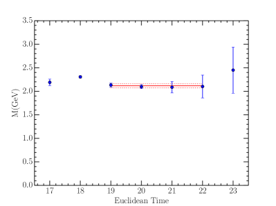
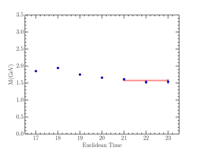
Figure 1: (Colour online). Typical effective mass fits for positive-parity (top) and negative-parity (bottom) nucleon excitations. The top plot shows a fit to the first positive-parity excitation of the $4\times 4$ correlation matrix obtained from basis 1 described in Table 1 of Section V. The fitted mass of 2.11(4) GeV is shown as a green circle for basis 1 in Fig. 4, and provides $\chi^{2}$/dof $=0.17$. The bottom plot shows a fit to the lowest-lying state in the negative-parity sector. It is sourced from the $6\times 6$ correlation matrix obtained from basis 3 described in Table 1 of Section V. The fitted mass of 1.58(3) GeV is shown as a blue square for basis 3 in Fig. 8, and corresponds to $\chi^{2}$/dof $=0.87$. Note, an earlier fit including $t=20$ provides $\chi^{2}$/dof $=1.22$, reflecting the systematic drift in the effective mass at early times.

As we will demonstrate, a careful covariance-matrix based $\chi^{2}$ analysis to fit the single-state ansatz ensures a robust extraction of the eigenstate energies. The physics underpinning this robustness is elucidated in detail in Section VI.

The CSSM lattice collaboration has used this technique in the calculation of the nucleon spectra in both the positive Mahbub et al. (2012) and negative-parity channels Mahbub et al. (2013a) with standard three-quark interpolators. While largely successful at identifying towers of excited states that would be associated with resonances in Nature, it has been shown that with three-quark operators alone it is difficult to detect states near multi-particle scattering energy levels Mahbub et al. (2014). The concern is that the operator basis doesn’t have sufficient overlap with meson-baryon type components, highlighting the need for studies with multi-hadron operators.

III Multi-particle State Contributions

In order to further elucidate the situation, we consider a simple two-component toy model which consists of two QCD energy eigenstates, $|\,a\rangle$ and $|\,b\rangle$. We then suppose that $|\,a\rangle$ and $|\,b\rangle$ are given by

$$\big{|}\,a\big{\rangle} =\;\;\,\cos\theta\,\big{|}\,1\big{\rangle}+\sin\theta\>\big{|}\,2\big{\rangle}\,,$$ (11)

$$\big{|}\,b\big{\rangle} =-\sin\theta\,\big{|}\,1\big{\rangle}+\cos\theta\,\big{|}\,2\big{\rangle}\,,$$ (12)

where $|\,1\rangle$ and $|\,2\rangle$ denote a single-hadron and meson-baryon type component respectively, while $\theta$ is some arbitrary mixing angle. Now imagine performing a spectroscopic calculation with an interpolating field $\chi_{3}$ that only has substantial overlap with $|\,1\rangle$. That is,

$$\big{\langle}\Omega\,\big{|}\,\chi_{3}\,\big{|}\,1\rangle\propto C\,\quad\mbox{and}\qquad\big{\langle}\Omega\,\big{|}\,\chi_{3}\,\big{|}\,2\rangle\ll C\,,$$ (13)

for some constant $C$. When $\overline{\chi}_{3}$ acts on the vacuum we therefore create a state that is superposition of the true energy eigenstates given by

$$\big{|}\,1\big{\rangle}=\cos\theta\,\big{|}\,a\big{\rangle}-\sin\theta\>\big{|}\,b\big{\rangle}\,.$$ (14)

In the absence of an operator that has substantial overlap with $|\,2\rangle$, it becomes impossible to separate out the true QCD eigenstates of interest. This naturally leads to two points of concern. Firstly, one cannot extract states with a significant $|\,2\rangle$ component and secondly there is possibly contamination of the states that are extracted. When performing baryon spectroscopy it therefore becomes desirable to include interpolating fields that we expect to have substantial overlap with multi-particle meson-baryon type states Lang and Verduci (2013). While projecting single-hadron momenta in a multi-hadron operator allows for a clean extraction of states associated with scattering thresholds, the influence of local five-quark operators (without explicit momenta assigned to each hadron) on the spectrum is less intuitive. It is the purpose of this study to examine the role local five-quark operators play in the spectrum, and to thereby test the robustness of our variational method.

Starting with standard $N$ and $\pi$ interpolators we use the Clebsch-Gordan coefficients to project isospin $I=1/2,I_{3}=+1/2$ and write down the general form of our meson-baryon interpolating fields Kiratidis et al. (2012); Kamleh et al. (2014),

$$\chi_{N\pi}(x) =\frac{1}{\sqrt{6}}\,\epsilon^{abc}\,\gamma_{5}\times$$

$$\quad\bigg{\{}2\big{[}u^{Ta}(x)\,\Gamma_{1}\,d^{b}(x)\big{]}\,\Gamma_{2}\,d^{c}(x)\,\big{[}\bar{d}^{e}(x)\,\gamma_{5}\,u^{e}(x)\big{]}$$

$$\quad-\big{[}u^{Ta}(x)\,\Gamma_{1}\,d^{b}(x)\big{]}\,\Gamma_{2}\,u^{c}(x)\,\big{[}\bar{d}^{e}(x)\,\gamma_{5}\,d^{e}(x)\,\big{]}$$

$$\quad+\big{[}u^{Ta}(x)\,\Gamma_{1}\,d^{b}(x)\big{]}\,\Gamma_{2}\,u^{c}(x)\,\big{[}\,\bar{u}(x)^{e}\,\gamma_{5}\,u^{e}(x)\big{]}\bigg{\}},$$ (15)

providing us with two five-quark operators, denoted $\chi_{5}$ and $\chi^{\prime}_{5}$ which correspond to $(\Gamma_{1},\Gamma_{2})=(C\gamma_{5},\textrm{I})$ and $(\Gamma_{1},\Gamma_{2})=(C,\gamma_{5})$ respectively. The square brackets around the diquark contraction denote a Dirac scalar. Under a parity transformation

$$x\rightarrow\tilde{x}=(x_{0},-\vec{x})\,,$$ (16)

and the quark fields $\psi(x)$ and $\bar{\psi}(x)$ transform as

$$\psi(x) \rightarrow\mathcal{P}\,\psi(x)\,\mathcal{P}^{\dagger}=\gamma_{0}\,\psi(\tilde{x})\,,$$

$$\bar{\psi}(x) \rightarrow\mathcal{P}\,\bar{\psi}(x)\,\mathcal{P}^{\dagger}=\bar{\psi}(\tilde{x})\,\gamma_{0}.$$ (17)

Applying a parity transformation to the standard pion interpolator $\chi_{\pi}(x)=\bar{\psi}(x)\gamma_{5}\psi(x)$, and the nucleon interpolators of type $\chi_{N}(x)=\big{[}\psi^{T}(x)(C\gamma_{5})\psi(x)\big{]}\psi(x)$ of Eq. (V) we find

$$\chi_{\pi}(x) \rightarrow-\bar{\psi}(\tilde{x})\,\gamma_{5}\,\psi(\tilde{x})=-\chi_{\pi}(\tilde{x})\,,$$

$$\chi_{N}(x) \rightarrow\big{[}\psi^{T}(\tilde{x})\,(C\gamma_{5})\,\psi(\tilde{x})\big{]}\gamma_{0}\,\psi(\tilde{x})=\gamma_{0}\,\chi_{N}(\tilde{x}).$$ (18)

Thus the pion interpolator transforms negatively under parity. To ensure our five-quark baryon interpolator formed from the product of pion and nucleon interpolators, transforms in the appropriate manner, the prefactor of $\gamma_{5}$ is included in Eq. (III). That is, both our three-quark and five-quark nucleon operators have the same parity transformation properties and hence can be combined in a correlation matrix. This also ensures the standard parity projector of Eq. (2) applies to our five-quark interpolators.

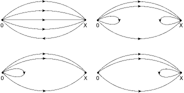
Figure 2: The Feynman diagrams considered following the introduction of five-quark interpolating fields to standard three-quark operators.

The presence of creation quark fields in our annihilation interpolating field and vice versa then leads to the requirement of calculating the more computationally intense loop propagators, in order to compute the diagrams in Fig. 2. The literature contains different ways of dealing with such diagrams such as distillation Peardon et al. (2009), and various schemes such as the Laplacian Heaviside (LapH) smearing method Morningstar et al. (2011). Here we will stochastically estimate inverse matrix elements fully diluting in spin, colour and time as outlined below.

IV Loop Propagator Techniques

As observed in the preceding section, spectroscopic calculations that involve the five-quark operators $\chi_{5}$ and $\chi_{5}^{\prime}$ necessarily involve the determination of loop propagators at $x,$ denoted $S(x,x)$. As $S(x,x)$ requires a source at each lattice point, a different recipe to that of conventional point-to-all propagators is utilised. For this purpose we use stochastic estimation of the matrix inverse Dong and Liu (1994); Foley et al. (2005).

Given a set of random noise vectors $\{\eta\}$ with elements drawn from $\mathbb{Z}_{4}$ such that the average over noise vectors gives

$$\langle\eta_{a\alpha}(x)\,\eta_{b\beta}^{\dagger}(y)\rangle=\delta_{xy}\,\delta_{ab}\,\delta_{\alpha\beta},$$ (19)

with colour indices $a,b$, spin indices $\alpha,\beta$ and space-time indices $x,y$. We define for each noise vector a corresponding solution vector

$$\chi=M^{-1}\,\eta,$$ (20)

where in this case $M$ is the fermion matrix. Then the stochastic estimate of a propagator matrix element is calculated as

$$S_{{ab};\alpha\beta}(x,y)\simeq\langle\chi_{a\alpha}(x)\,\eta_{b\beta}^{\dagger}(y)\rangle.$$ (21)

We perform full dilution in time, spin and colour indices as a means of variance reduction O’Cais et al. (2004). That is, given a set of full noise vectors $\{\eta\},$ we can define a set of diluted noise vectors $\{\eta^{[a^{\prime}\alpha^{\prime}t^{\prime}]}\}$ by

$$\eta^{[a^{\prime}\alpha^{\prime}t^{\prime}]}_{a\alpha}(\vec{x},t)=\delta_{aa^{\prime}}\,\delta_{\alpha\alpha^{\prime}}\,\delta_{tt^{\prime}}\,\eta_{a\alpha}(\vec{x},t),$$ (22)

where the intrinsic quark field indices are specified by colour $a,$ spin $\alpha,$ space $\vec{x}$ and time $t$ respectively and the colour-spin-time diluted noise vectors are enumerated by the corresponding $[a^{\prime}\,\alpha^{\prime}\,t^{\prime}]$ labels. We can similarly enumerate the solution vectors

$$\chi^{[a^{\prime}\alpha^{\prime}t^{\prime}]}=M^{-1}\eta^{[a^{\prime}\alpha^{\prime}t^{\prime}]},$$ (23)

which makes it clear that by diluting we increase the number of inversions required by a factor of $n_{\rm colour}\times n_{\rm spin}\times n_{\rm time}.$ The stochastic estimate of the matrix inverse with dilution is given by

$$S(x,y)\simeq\langle\sum_{a^{\prime},\alpha^{\prime},t^{\prime}}\chi^{[a^{\prime}\alpha^{\prime}t^{\prime}]}(x)\,\eta^{[a^{\prime}\alpha^{\prime}t^{\prime}]\dagger}(y)\,\rangle,$$ (24)

where colour and spin indices are taken to be implicit for clarity. At this point we remark that, while it is computationally infeasible to also fully dilute in the space index $\vec{x},$ in this extreme limit each diluted noise vector would consist of only a single non-zero element, meaning that we are exactly calculating the full matrix $S(x,y)$ and the above relation becomes an equality rather than an estimate. This makes it clear that using dilution provides an improved stochastic estimate to the matrix inverse.

As shown in Fig. 2, our construction of nucleon correlators with five-quark operators combines standard point-to-all propagators $S(x,0)$ and stochastic estimates of the loop propagators $S(x,x).$ In order to access the radial excitations of the nucleon, we make use of multiple levels of Gaussian smearing in our quark fields. Hence, to construct a correlation matrix we need to calculate propagators with differing levels of source and sink smearing.

Let $S^{(m,n)}(x,y)$ denote a propagator with $m$ iterations of smearing applied at the sink and $n$ iterations applied at the source. In the case of point-to-all propagators $S^{(m,n)}(x,0)$ the source point is fixed, $y=0,$ and starting with a point source $\psi^{(0)},$ we apply $n$ iterations of Gaussian smearing pre-inversion to obtain the smeared source $\psi^{(n)}=H^{n}\,\psi^{(0)},$ where

$$H\,\psi(x)=(1-\alpha)\,\psi(x)+\frac{\alpha}{6}\sum_{\mu=1}^{3}\left\{U_{\mu}(x)\,\psi(x+a\hat{\mu})\right.\\ \left.+U^{\dagger}_{\mu}(x-a\hat{\mu})\,\psi(x-a\hat{\mu})\right\},$$ (25)

and $\alpha$ specifies the smearing fraction. Sink smearing is applied to the propagator post-inversion to obtain $S^{(m,n)}(x,0).$

The application of smearing to construct a stochastic estimate for the quark propagator $S^{(m,n)}(x,y)$ is somewhat different. The set of (diluted) noise and solution vectors $\{\eta,\chi\}$ is first constructed, whereby it follows from Eqs. (21) and (25) that an estimate of the smeared propagator is given by

$$S^{(m,n)}(x,y)=\langle\chi^{(m)}(x)\eta^{(n)\dagger}(y)\rangle,$$ (26)

where $\chi^{(m)}=H^{m}\chi$ is the result of $m$ iterations of Gaussian smearing applied to the (diluted) solution vectors, and $\eta^{(n)}=H^{n}\eta$ is similarly constructed from the (diluted) noise vectors. Note that the smearing is applied after (any dilution and) the solution vectors have been calculated. The construction of a smeared loop propagator $S^{(m,m)}(x,x)$ is simply an application of the above formulae in the case $y=x.$

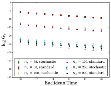
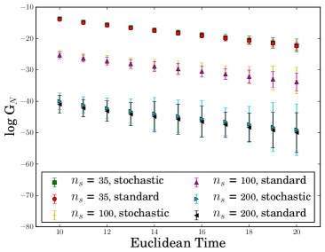
Figure 3: (Colour online). A comparison of correlators calculated with one stochastically estimated propagator (denoted “stochastic”) to those calculated with no stochastic propagators (denoted “standard”). Results are presented for the pion (top) and the ground state nucleon (bottom).

In order to determine how many noise vectors per configuration are sufficient to provide similar statistical errors for our point-to-all and stochastic propagators, correlators are calculated with a stochastic estimate of the point-to-all propagator, and compared to those obtained using point-to-all propagators calculated in the standard way. As each independent quark line in a hadron correlator requires an independent noise source to ensure unbiased estimation Morningstar et al. (2011) we insert one stochastic propagator into the aforementioned correlators. Furthermore, as a test of our smearing technique for stochastic propagators, we perform this comparison using a variety of smearing levels. Note that, as smearing of both the source and solution vectors is performed post-inversion, the stochastic method effectively provides different smearing levels for free.

The comparison is performed on 75 $20^{3}\times 40$ lattice gauge configurations, with the FLIC fermion action Zanotti et al. (2002). The lattice spacing is $0.126\textrm{ fm}$ in both the temporal and spatial direction providing a physical lattice volume of $(2.52\textrm{ fm})^{3}$. Four full noise vectors are used per stochastic propagator, which are then colour-spin-time diluted. As the source timeslice is fixed in this case, each stochastic propagator requires $n_{\rm colour}\times n_{\rm spin}$ inversions per noise vector. Recall standard point-to-all propagators require $n_{\rm colour}\times n_{\rm spin}$ inversions, although source smearing is applied pre-inversion unlike the stochastic case. Three different levels of smearing are used, $n_{s}=35,100,200$ sweeps with $\alpha=0.7.$ Fig. 3 shows good agreement across all smearing levels between those correlators containing a stochastically estimated propagator and those that do not, demonstrating that using four noise vectors per quark line provides a comparable statistical uncertainty to that of a standard propagator. We note here that ultimately we utilise this method to calculate $S(x,x)$ not $S(x,x_{source}),$ meaning we get the added benefit of spatial averaging for our loop propagators.

V Simulation Details

For the baryon spectroscopy results presented herein we use the PACS-CS $2+1$ flavour dynamical-fermion configurations Aoki et al. (2009) made available through the ILDG Beckett et al. (2011). These configurations use the non-perturbatively $\mathcal{O}(a)$-improved Wilson fermion action and the Iwasaki gauge action Iwasaki (1983). The lattice size is $32^{3}\times 64$ with a lattice spacing of $0.0907\textrm{ fm}$ providing a physical volume of $\approx(2.90\textrm{ fm})^{3}$. $\beta=1.90$, the light quark mass is set by the hopping parameter $\kappa_{ud}=0.13770$ which gives a pion mass of $m_{\pi}=293\textrm{ MeV}$, while the strange quark mass is set by $\kappa_{s}=0.13640$. Fixed boundary conditions are employed in the time direction removing backward propagating states Melnitchouk et al. (2003); Mahbub et al. (2009b), and the source is inserted at $t_{src}=n_{t}/4=16$, well away from the boundary. Systematic effects associated with this boundary condition are negligible for $t>16$ slices from the boundary. The main results of our variational analysis is performed at $t_{0}=17$ and $dt=3,$ providing a good balance between systematic and statistical uncertainties. Uncertainties are obtained via single elimination jackknife while a full covariance matrix analysis provides the $\chi^{2}/dof$ which is utilised to select fit regions for the eigenstate-projected correlators.

In addition to the five quark operators $\chi_{5}$ and $\chi_{5}^{\prime}$ presented in Section III we use the conventional three-quark operators

$$\chi_{1} =\epsilon^{abc}[u^{aT}\,(C\gamma_{5})\,d^{b}]\,u^{c}$$

$$\chi_{2} =\epsilon^{abc}[u^{aT}\,(C)\,d^{b}]\,\gamma_{5}\,u^{c}$$ (27)

in order to form the seven bases we study that are outlined in Table 1.

Table 1: Table of the various operators used in each basis.

Basis Number	Operators Used
1	$\chi_{1}$, $\chi_{2}$
2	$\chi_{1}$, $\chi_{2}$, $\chi_{5}$
3	$\chi_{1}$, $\chi_{2}$, $\chi_{5}^{\prime}$
4	$\chi_{1}$, $\chi_{2}$, $\chi_{5}$, $\chi_{5}^{\prime}$
5	$\chi_{1}$, $\chi_{5}$, $\chi_{5}^{\prime}$
6	$\chi_{2}$, $\chi_{5}$, $\chi_{5}^{\prime}$
7	$\chi_{5}$, $\chi_{5}^{\prime}$

Throughout this work we employ Gauge-invariant Gaussian smearing Gusken (1990) at the source and sink to increase the basis size via altering the overlap of our operators with the states of interest. We choose $n_{s}=35$ and $n_{s}=200$ sweeps of smearing providing bases of sizes 4, 6 and 8. Stochastic quark lines are calculated using four random $\mathbb{Z}_{4}$ noise vectors that are fully diluted in colour, spin and time.

VI Results

VI.1 Positive-parity Spectrum

The results for the nucleon spectrum in the positive-parity sector are shown in Fig. 4. Solid horizontal lines are added to guide the eye, with their values set by the states in basis number 4, since this basis contains all the operators studied and has the largest span.

Of particular interest is the robustness of the variational techniques employed. While changing bases may effect whether or not a particular state is seen, the energy of the extracted states is consistent across the different bases, even though they contain qualitatively different operators.

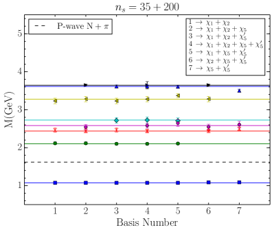
Figure 4: (Colour online). The positive-parity nucleon spectrum with various operator bases constructed with 35 and 200 sweeps of smearing. Horizontal solid lines are present to guide the eye and are drawn from the central value of the states in basis 4, while the dashed line marks the position of the non-interacting P-wave $N\pi$ scattering threshold

.

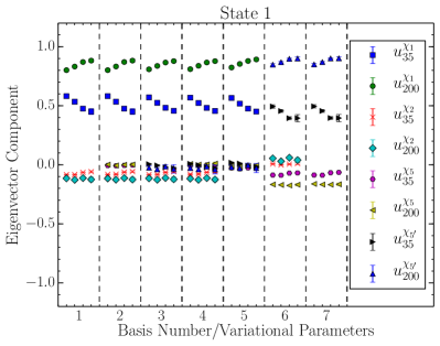
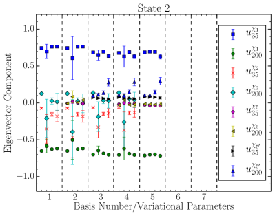
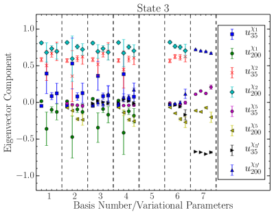
Figure 5: (Colour online). Eigenvector components corresponding to the low-lying positive-parity nucleon states. State 1 corresponds to the ground state, with states 2 and 3 corresponding to the first and second excited states respectively. The column numbers denote basis number while the minor $x$ axis ticks correspond to the values of the variational parameter $dt$ which runs from 1 through to 4. $t_{0}=17$ has been used throughout. The subscripts 35 and 200 in the legend refer to the number of smearing sweeps applied.

Despite the use of 5-quark operators, no state near the non-interacting P-wave $N\pi$ scattering threshold is observed. This is understood by noting that none of our operators have a source of the back-to-back relative momentum between the nucleon and pion necessary to observe an energy level in the region of this scattering state.

The corresponding eigenvector components for the positive-parity states are shown in Fig. 5 as a function of basis and variational parameter $dt,$ with $t_{0}=17$ fixed. The values of $dt$ range from 1 through 4. The upper limit of $dt=4$ was chosen as the largest value for which the variational analysis converged for each of the seven bases.

The ground-state nucleon is observed in every basis regardless of the absence or presence of a particular operator. If $\chi_{1}$ is present then this provides the dominant contribution, with $\chi_{5}^{\prime}$ coupling strongly to the ground state in bases where $\chi_{1}$ is absent. An interesting interplay between 35 and 200 sweep smeared $\chi_{1}$ is observed with the smaller source diminishing in importance as $dt$ is increased. This may be associated with the Euclidean time evolution of highly excited states which are suppressed with increasing $dt$.

Turning our attention to state 2, we see that $\chi_{1}$ plays a critical role in the extraction of the first excited state, which is associated with a radial excitation of the ground state Roberts et al. (2014). Here the 35 and 200 sweep $\chi_{1}$ interpolators enter with similar strength but opposite signs, setting up the node structure of a radial excitation. $\chi_{1}$ dominates the construction of the optimised operator for this state for bases 1 through 5, whereas basis 6 and 7 which lack $\chi_{1}$ do not observe this state.

The eigenvectors for state 3, the second excited state, are dominated by $\chi_{2}$ components with the same sign when this operator is present (bases 1-4,6). This state is not observed in basis 5 (where $\chi_{2}$ is absent). Interestingly, in basis 7 which only contains five-quark operators it appears that it is possible to form this state using $\chi_{5}^{\prime}$ components at two different smearings with opposite sign.

We observe that the overall structure of the eigenvectors for each of the three states is highly consistent across different bases and different values of the variational parameter $dt.$ The structure of the eigenvectors can be considered to be a signature or fingerprint of the extracted state, and this consistency across bases confirms that it is the same state being identified.

It is fascinating to see that for state 1 in bases 6 and 7, where $\chi_{5}^{\prime}$ takes the role of the absent $\chi_{1}$ operator, the values of the two dominant eigenvector components (which indicate the mixture of the two different smearing levels used) are extremely similar to the $\chi_{1}$ components in bases 1-5. Interestingly, at $dt=2$ the error bars for the dominant components of states 2 and 3 blow up. As we shall explain below, this is due to an accidental degeneracy in the eigenmasses for this choice of variational parameters.

In order to further test the robustness of our variational method we conduct a comparison of the masses obtained from fitting the eigenstate-projected correlators as a function of the variational parameters for each basis. These results are presented in Fig. 6. Also shown for comparison are the eigenmasses, $m_{\alpha}$, that result from solving the generalised eigenvalue equation of Eqs. (7) or (8) with $c^{\alpha}=\textrm{e}^{-m_{\alpha}dt}$.

Studying state 1, the nucleon ground state, we observe that the masses obtained from projected correlator fits are approximately invariant across different bases and choices of the variational parameter. In contrast, the eigenmass lies well above the fitted mass, dropping in value as the variational parameter $dt$ is varied from 1 to 4. While the eigenmass is directly related to the principal correlator and thus should approach the ground state mass in the large time limit, it is clear that the values of $dt$ we examine here are insufficient for this to occur. It is worth noting that, in bases 6 and 7 where $\chi_{1}$ is absent we see that the eigenmass value rises significantly. Nevertheless, the fitted mass remains remarkably consistent with the values obtained in bases 1-5. We emphasize how strong the variational parameter dependence of the eigenmass contrasts the more consistent structure of the eigenvectors. Insensitivity of the eigenvectors to the variational parameters is a key component of the invariance of the masses obtained from the projected correlator.

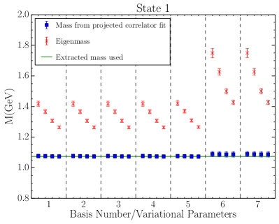
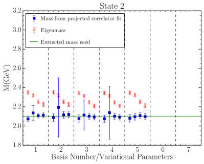
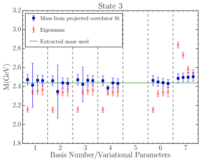
Figure 6: (Colour online). Comparisons of eigenmasses to masses obtained from a projected correlator fit for low-lying states in the positive-parity nucleon channel. The column numbers denote basis number while the minor $x$ axis ticks correspond to the values of the variational parameter $dt=1\ldots 4.$ $t_{0}=17$ has been used throughout. The line denoting the extracted mass is set using basis 4 with $dt=3.$

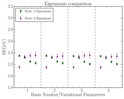
Figure 7: (Colour online). A plot showing the eigenmasses for both states 2 and 3, illustrating the accidental degeneracy at $dt=2$.

Turning to state 2, we see that the eigenmass shows similar behaviour to state 1, lying above the extracted mass and dropping with $dt.$ Interestingly, for state 3 in bases 1-4 and 6 the eigenmass shows constant behaviour for $dt=2-4$ but systematically lies below the extracted mass. In basis 7, the state 3 eigenmass is very different to the previous bases, lying above the extracted mass and showing a similar downward trend to states 1 and 2 as $dt$ varies.

As for state 1, the fitted masses for states 2 and 3 provide highly consistent values and uncertainties across the different bases and values of $dt,$ with the notable exception of $dt=2.$ As observed previously in Fig. 5, we see in Fig. 6 considerably larger error bars at the variational parameter set $(t_{0},dt)=(17,2)$ in both the eigenvector components and projected mass fits for the first and second excited states. To understand this, we turn to Fig. 7, where the eigenmasses for states 2 and 3 are plotted against the variational parameter $dt$ in each basis.

Note that at $(t_{0},dt)=(17,2)$ there is an approximate degeneracy in the eigenmass for states 2 and 3. As a consequence, the corresponding eigenvectors can therefore be arbitrarily rotated within the state 2/state 3 subspace while remaining a solution to the eigenvalue problem. When constructing the jackknife sub-ensembles to calculate the error in the fitted energy, we need to solve for the eigenvectors on each sub-ensemble. Due to the approximate degeneracy, the particular linear combination of state 2 and state 3 that we obtain for each sub-ensemble can vary. Indeed, we observe that the dot-product between the ensemble average and sub-ensemble can drop significantly for $dt=2$ in comparison to other values of $dt.$ This causes a large variation in the sub-ensemble eigenvector components and a correspondingly large error bar. The simplest way to avoid the problem of this accidental degeneracy is to select a different value of the variational parameter.

VI.2 Negative-parity Spectrum

The negative-parity nucleon spectrum is presented in Fig. 8. Solid horizontal lines have been added to guide the eye, with their values set by the states in the largest basis (number 4). Once again, while changing bases effects whether or not we observe a given state, the extracted states display an impressive level of consistency across the different bases.

The dashed line indicating the energy of the non-interacting (infinite-volume) scattering-state threshold is also indicated with the caution that mixing with nearby states in the finite volume can alter the threshold position Hall et al. (2013); Menadue et al. (2012). We note here that all scattering thresholds discussed in this section and the next, refer to the non-interacting threshold. In contrast to the positive-parity results, we do observe a state near the S-wave $N\pi$ scattering threshold in the negative-parity channel (bases 5,6,7), also noting that the P-wave $N\pi\pi$ thresholds lie in the region of state 3 seen in bases 3, 4 and 5. It is important to note that even after the introduction of operators that permit access to a state near the low-lying scattering state, the energies of the higher states in the spectrum are consistent, demonstrating the robustness of the variational techniques employed.

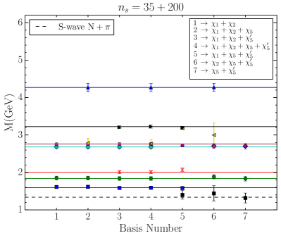
Figure 8: (Colour online). The negative-parity nucleon spectrum with various operator bases using 35 and 200 sweeps of smearing. Solid horizontal lines are present to guide the eye and are drawn from the central value of the states in basis 4, since this basis is the largest. The dashed line marks the position of the non-interacting S-wave $N\pi$ scattering threshold. The variational parameters used herein are $(t_{0},dt)=(17,3)$.

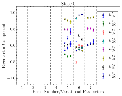
Figure 9: (Colour online). Eigenvector components corresponding to State 0 which is in the region of the non-interacting S-wave $N+\pi$ scattering threshold. The column numbers denote basis number while the minor $x$ axis ticks correspond to the values of the variational parameter $dt$ which runs from 1 through to 3. $t_{0}=17$ has been used throughout. The subscripts 35 and 200 in the legend refer to the number of smearing sweeps applied.

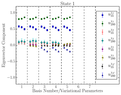
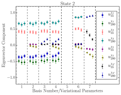
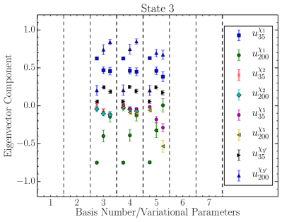
Figure 10: (Colour online). Eigenvector components corresponding to low-lying negative-parity nucleon states. States 1 and 2 correspond to the two lowest-lying resonant states, while state 3 interestingly lies in the region of the P-wave scattering thresholds. The column numbers denote basis number while the minor $x$ axis ticks correspond to the values of the variational parameter $dt$ which runs from 1 through to 3. $t_{0}=17$ has been used throughout. The subscripts 35 and 200 in the legend refer to the number of smearing sweeps applied.

Plots of the corresponding eigenvectors for the low-lying negative-parity states as a function of basis and variational parameter $dt=1\ldots 3$ are presented in Figures  9 and  10. The upper limit of $dt=3$ was chosen as the largest value for which the variational analysis converged for all seven bases. The eigenvector components for state 0 (when it is present) are dominated by the multi-particle operators $\chi_{5}$ and $\chi_{5}^{\prime},$ suggesting that this state should be identified as a scattering state. The extracted energy for this state is in the region of the non-interacting S-wave $N\pi$ scattering threshold (which lies below the first negative-parity resonant state). The uncertainty in bases 6 and 7 are relatively large compared to basis 5, indicating that the presence of $\chi_{1}$ may also be required to cleanly isolate this scattering state. Indeed, we note that in basis 5 there is a significant contribution to state 0 from the $\chi_{1}{(n_{s}=200)}$ operator.

It is also important to note that either $\chi_{5}$ or $\chi_{5}^{\prime}$ can be the dominant interpolator exciting this lowest-lying state. Given that $\chi_{2}$ is predominantly associated with the third state in the positive-parity sector at 2.4 GeV one might naively expect $\chi_{5}^{\prime}$ would be associated with S-wave scattering states near 2.7 GeV. Remarkably it creates a scattering state near 1.35 GeV. Thus one should use caution in predicting the spectral overlap of five-quark operators by examining the spectral overlap of the pion and nucleon components of the five-quark operators separately. In light of the quark field operator contractions required in calculating the full two-point function this result is not surprising.

In accord with previous studies Mahbub et al. (2013a, b), we find that the $\chi_{1}$ interpolating field is crucial for extracting state 1, associated with the lowest-lying negative-parity resonance, as we do not observe this state when $\chi_{1}$ is absent as in bases 6 and 7. As expected, $\chi_{1}$ provides the dominant contribution to state 1, which is associated with the $S_{11}(1535)$ in Nature. Similarly, we see that $\chi_{2}$ has a high overlap with state 2, the next resonant state. Basis 5 does not see state 2 due to the absence of $\chi_{2}$. However, unlike state 1, there is an important mixing of $\chi_{1}$ and $\chi_{2}$ in isolating the eigenstate. It is interesting to note that in basis 7 we are able to form this state by combining $\chi_{5}$ and $\chi_{5}^{\prime}.$

The consistency of the eigenvector structure for the low-lying states 1 and 2 is strong. Despite the appearance of a state near the S-wave $N\pi$ threshold, state 0 in basis 5, the eigenvector components for state 1 are remarkably consistent with those in other bases where this lower-lying state is absent. If we look at basis 6, where state 0 is present but state 1 is absent, the eigenvector components for state 2 are in good agreement with those from other bases where the lower-lying state 0 is not observed. This demonstrates that, with a judiciously chosen variational technique, a reliable analysis of higher states in the spectrum can be performed even if states associated with the low-lying scattering states are not extracted by the correlation matrix analysis.

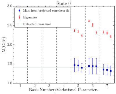
Figure 11: (Colour online). Comparisons of eigenmasses to masses obtained from a projected correlator fit for state 0, which is in the region of the non-interacting S-wave $N\pi$ scattering threshold. The column numbers denote basis number while the minor $x$ axis ticks correspond to the values of the variational parameter $dt=1\ldots 3.$ $t_{0}=17$ has been used throughout. The line denoting the extracted mass used has been set using basis 5 with $dt=3.$

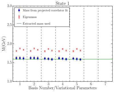
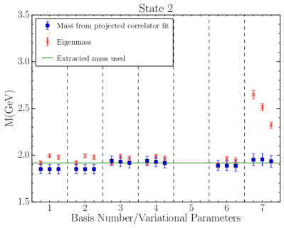
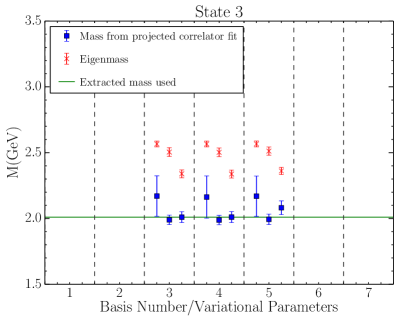
Figure 12: (Colour online). Comparisons of eigenmasses to masses obtained from a projected correlator fit for low lying states in the negative-parity nucleon channel. The column numbers denote basis number while the minor $x$ axis ticks correspond to the values of the variational parameter $dt=1\ldots 3.$ $t_{0}=17$ has been used throughout. The line denoting the extracted mass used has been set using basis 4 with $dt=3.$

State 3, which lies in the region of the non-interacting P-wave $N\pi\pi$ scattering states in the channel, also shows good agreement across bases and variational parameters. The dominant eigenvector components show that this state is formed from a mix of $\chi_{5}^{\prime}$ and $\chi_{1}.$ It is worth noting that very early choices of the variational parameters such as $(t_{0},dt)=(17,1)$ do not allow sufficient Euclidean time evolution to cleanly isolate this state. The correlation matrix has more states participating in the analysis than the dimension of the basis leading to contamination from unwanted states and hence spurious results. The different structure for the state 3 eigenvectors at these early variational parameter sets illustrates the need to allow sufficient Euclidean time evolution to occur.

The comparison of the fitted masses as a function of variational parameter $dt$ across the different bases for the negative-parity sector is shown in Figures 11 and 12. Again, the eigenmasses are plotted for comparison. As before, we observe for all the states the fitted masses are consistent across the different bases and values of $dt$. In contrast, the eigenmasses for the negative-parity states all show some variation with $dt$ to different extents, with the values typically lying well above the extracted energies.

Finally, we observe that whenever $\chi_{5}^{\prime}$ is present, either a state near the S-wave $N\pi$ scattering threshold, or a state lying in the region of the P-wave $N\pi\pi$ scattering thresholds is extracted. This indicates the presence of the vector di-quark in the interpolator may play an important role in scattering state excitation. It is perhaps surprising that basis 4 fails to see a state near the lowest-lying scattering threshold in the sector, despite being the largest basis. We believe this is due to the spectral strength available to the scattering state being relatively low. The overlap of the scattering state with the operators is not high enough to compete with the large spectral strength imparted to the low-lying resonant states when both $\chi_{1}$ and $\chi_{2}$ are present. We note that the only time our local (three-quark or five-quark) operators overlap with a meson-baryon state is when both hadrons are at the origin. The probability of this occurring is proportional to $1/V^{2}.$ After taking into account the spatial sum in Eq. 1, this results in a $1/V$ suppression of multi-particle states in the correlator amplitude $\mathcal{G}(t)$ Luscher (1991). Indeed, it seems to be relatively difficult to extract a state near the S-wave $N\pi$ state with our local five-quark operators, suggesting that scattering state excitation is best achieved by explicitly projecting the momentum of interest onto each hadron present in the scattering state.

VII Conclusions

We have investigated the role of local multi-particle interpolators in calculating the nucleon spectrum by examining a variety of different bases both with and without five-quark operators.

The variational techniques herein employed, demonstrate that fitting a single-state ansatz to optimised eigenstate-projected correlators provides a method to reliably extract energies in both the positive and negative-parity channels. While the selection of states that are observed varied between bases, when a given state is seen the extracted energy agrees across qualitatively different bases.

Furthermore, the structure of the eigenvector components and the corresponding fitted energies for the states observed are shown to be highly consistent across different bases and choices of the variational parameters, despite the markedly different interpolators used in the various bases. We found that an approximate accidental degeneracy in the eigenmass at $(t_{0},dt)=(17,2)$ for states 2 and 3 led to a large increase in the uncertainties for the corresponding energies and eigenvector components.

While we did not observe any positive-parity scattering states, in the negative-parity sector we found that $\chi_{5}^{\prime}$ was crucial to obtaining an energy in the region of the non-interacting S-wave $N\pi$. Even with the use of local five-quark interpolators the uncertainties on this threshold state were relatively large compared to those of higher states. Future studies will include multi-particle operators with explicitly projected single-hadron momenta in the variational basis to facilitate better excitation of scattering states, including those in the positive-parity sector. An interesting feature of our negative-parity results is that the energies of the extracted states are consistent across all bases in which the state is observed, regardless of the presence (or not) of a state in the region of the lower-lying non-interacting scattering threshold. This suggests that by using the techniques described herein, one does not need to have access to the aforementioned low-lying states to reliably extract energies closely related to the resonances of Nature.

References

- Michael (1985) C. Michael, Nucl.Phys. B259, 58 (1985).
- Luscher and Wolff (1990) M. Luscher and U. Wolff, Nucl.Phys. B339, 222 (1990).
- Liu et al. (2014) K.-F. Liu, Y. Chen, M. Gong, R. Sufian, M. Sun, et al., PoS LATTICE2013, 507 (2014), arXiv:1403.6847 [hep-ph] .
- Roberts et al. (2013) D. S. Roberts, W. Kamleh, and D. B. Leinweber, Physics Letters B 725, 164 (2013), arXiv:1304.0325 [hep-lat] .
- Bauer et al. (2012) T. Bauer, J. Gegelia, and S. Scherer, Phys.Lett. B715, 234 (2012), arXiv:1208.2598 [hep-ph] .
- Edwards et al. (2011) R. G. Edwards, J. J. Dudek, D. G. Richards, and S. J. Wallace, Phys.Rev. D84, 074508 (2011), arXiv:1104.5152 [hep-ph] .
- Roberts et al. (2012) C. D. Roberts, I. C. Cloet, L. Chang, and H. L. Roberts, AIP Conf.Proc. 1432, 309 (2012), arXiv:1108.1327 [nucl-th] .
- Mahbub et al. (2012) M. S. Mahbub, W. Kamleh, D. B. Leinweber, P. J. Moran, and A. G. Williams, Phys.Lett. B707, 389 (2012), arXiv:1011.5724 [hep-lat] .
- Isgur and Karl (1977) N. Isgur and G. Karl, Phys.Lett. B72, 109 (1977).
- Isgur and Karl (1979) N. Isgur and G. Karl, Phys.Rev. D19, 2653 (1979).
- Glozman and Riska (1996) L. Y. Glozman and D. Riska, Phys.Rept. 268, 263 (1996), arXiv:hep-ph/9505422 [hep-ph] .
- Speth et al. (2000) J. Speth, O. Krehl, S. Krewald, and C. Hanhart, Nucl.Phys. A680, 328 (2000).
- Burch et al. (2004) T. Burch et al., Phys.Rev. D70, 054502 (2004), arXiv:hep-lat/0405006 [hep-lat] .
- Mahbub et al. (2010) M. Mahbub, A. O. Cais, W. Kamleh, D. B. Leinweber, and A. G. Williams, Phys.Rev. D82, 094504 (2010), arXiv:1004.5455 [hep-lat] .
- Mahbub et al. (2013a) M. S. Mahbub, W. Kamleh, D. B. Leinweber, P. J. Moran, and A. G. Williams, Phys.Rev. D87, 011501 (2013a), arXiv:1209.0240 [hep-lat] .
- Mahbub et al. (2009a) M. Mahbub, A. O. Cais, W. Kamleh, B. G. Lasscock, D. B. Leinweber, et al., Phys.Lett. B679, 418 (2009a), arXiv:0906.5433 [hep-lat] .
- Roberts et al. (2014) D. S. Roberts, W. Kamleh, and D. B. Leinweber, Phys.Rev. D89, 074501 (2014), arXiv:1311.6626 [hep-lat] .
- Bruns et al. (2011) P. C. Bruns, M. Mai, and U. G. Meissner, Phys.Lett. B697, 254 (2011), arXiv:1012.2233 [nucl-th] .
- Lang and Verduci (2013) C. Lang and V. Verduci, Phys.Rev. D87, 054502 (2013), arXiv:1212.5055 .
- Mahbub et al. (2014) M. S. Mahbub, W. Kamleh, D. B. Leinweber, and A. G. Williams, Annals Phys. 342, 270 (2014), arXiv:1310.6803 [hep-lat] .
- Morningstar et al. (2013) C. Morningstar, J. Bulava, B. Fahy, J. Foley, Y. Jhang, et al., Phys.Rev. D88, 014511 (2013), arXiv:1303.6816 [hep-lat] .
- (22) M. S. Mahbub, Excitations of the nucleon in lattice QCD, PhD. Thesis, University of Adelaide .
- Kiratidis et al. (2012) A. L. Kiratidis, W. Kamleh, and D. B. Leinweber, PoS LATTICE2012, 250 (2012), arXiv:1301.3591 [hep-lat] .
- Kamleh et al. (2014) W. Kamleh, A. L. Kiratidis, and D. B. Leinweber, (2014), arXiv:1411.7119 [hep-lat] .
- Peardon et al. (2009) M. Peardon et al. (Hadron Spectrum Collaboration), Phys.Rev. D80, 054506 (2009), arXiv:0905.2160 [hep-lat] .
- Morningstar et al. (2011) C. Morningstar, J. Bulava, J. Foley, K. J. Juge, D. Lenkner, et al., Phys.Rev. D83, 114505 (2011), arXiv:1104.3870 [hep-lat] .
- Dong and Liu (1994) S.-J. Dong and K.-F. Liu, Phys.Lett. B328, 130 (1994), arXiv:hep-lat/9308015 [hep-lat] .
- Foley et al. (2005) J. Foley, K. Jimmy Juge, A. O’Cais, M. Peardon, S. M. Ryan, et al., Comput.Phys.Commun. 172, 145 (2005), arXiv:hep-lat/0505023 [hep-lat] .
- O’Cais et al. (2004) A. O’Cais, K. J. Juge, M. J. Peardon, S. M. Ryan, and J.-I. Skullerud, , 844 (2004), arXiv:hep-lat/0409069 [hep-lat] .
- Zanotti et al. (2002) J. M. Zanotti et al. (CSSM Lattice Collaboration), Phys.Rev. D65, 074507 (2002), arXiv:hep-lat/0110216 [hep-lat] .
- Aoki et al. (2009) S. Aoki et al. (PACS-CS Collaboration), Phys.Rev. D79, 034503 (2009), arXiv:0807.1661 [hep-lat] .
- Beckett et al. (2011) M. G. Beckett, B. Joo, C. M. Maynard, D. Pleiter, O. Tatebe, et al., Comput.Phys.Commun. 182, 1208 (2011), arXiv:0910.1692 [hep-lat] .
- Iwasaki (1983) Y. Iwasaki, (1983).
- Melnitchouk et al. (2003) W. Melnitchouk, S. O. Bilson-Thompson, F. Bonnet, J. Hedditch, F. Lee, et al., Phys.Rev. D67, 114506 (2003), arXiv:hep-lat/0202022 [hep-lat] .
- Mahbub et al. (2009b) M. Mahbub, A. O. Cais, W. Kamleh, B. Lasscock, D. B. Leinweber, et al., Phys.Rev. D80, 054507 (2009b), arXiv:0905.3616 [hep-lat] .
- Gusken (1990) S. Gusken, Nucl.Phys.Proc.Suppl. 17, 361 (1990).
- Hall et al. (2013) J. Hall, A. C. P. Hsu, D. Leinweber, A. Thomas, and R. Young, Phys.Rev. D87, 094510 (2013), arXiv:1303.4157 [hep-lat] .
- Menadue et al. (2012) B. J. Menadue, W. Kamleh, D. B. Leinweber, and M. S. Mahbub, Phys.Rev.Lett. 108, 112001 (2012), arXiv:1109.6716 [hep-lat] .
- Mahbub et al. (2013b) M. S. Mahbub, W. Kamleh, D. B. Leinweber, P. J. Moran, and A. G. Williams, Phys.Rev. D87, 094506 (2013b), arXiv:1302.2987 [hep-lat] .
- Luscher (1991) M. Luscher, Nucl.Phys. B364, 237 (1991).