Optimal strategies of investment in a linear stochastic model of market

Abstract.

We study the continuous time portfolio optimization model on the market where the mean returns of individual securities or asset categories are linearly dependent on underlying economic factors. We introduce the functional $Q_{\gamma}$ featuring the expected earnings yield of portfolio minus a penalty term proportional with a coefficient $\gamma$ to the variance when we keep the value of the factor levels fixed. The coefficient $\gamma$ plays the role of a risk-aversion parameter. We find the optimal trading positions that can be obtained as the solution to a maximization problem for $Q_{\gamma}$ at any moment of time. The single-factor case is analyzed in more details. We present a simple asset allocation example featuring an interest rate which affects a stock index and also serves as a second investment opportunity. We consider two possibilities: the interest rate for the bank account is governed by Vasicek-type and Cox-Ingersoll-Ross dynamics, respectively. Then we compare our results with the theory of Bielecki and Pliska where the authors employ the methods of the risk-sensitive control theory thereby using an infinite horizon objective featuring the long run expected growth rate, the asymptotic variance, and a risk-aversion parameter similar to $\gamma$.

1. Introduction

The art of making decisions about investment mix in order to meet specified investment goals for the benefit of the investors and balancing risk against performance is called the portfolio management (portfolio is a collection of investments all owned by the same individual or organization).

A modern study of portfolio selection begins in works by Markowitz [28], [29]. He showed how to formulate the problem of minimizing a portfolio’s variance subject to the constraint that its expected return equals a prescribed level as a quadratic program. Such an optimal portfolio is said to be variance minimizing and if it also achieves the maximum expected return among all portfolios having the same variance of return then it is said to be efficient [37].

There has been considerable research involving stochastic processes models of assets taking into account optimal investment decisions. Several researchers (e.g. Merton [31], Karatzas [25]) used stochastic control theory to develop continuous time portfolio management model where the assets are modeled bas stochastic processes but financial and economic factors are ignored. At the same time, a number of empirical studies (e.g.[34], [33], [20]) provided evidences that macroeconomic factors such as unemployment rate, inflation rate, dividend yield, change of industrial production, an interest rate, etc, influence on the stock return.

Lucas [27] introduced a discrete time model including stochastic process models as factors. Brennan, Schwartz and Lagnado [7] considered the factors as diffusion processes and assets as correlated Brownian motions, with the drift and diffusion coefficients for the asset pricesses taken to be deterministic functions of the factor levels. Their objective was to maximize expected utility of wealth at a terminal date. A key limitation of the Brennan-Schwartz-Lagnado approach is that one is unlikely to obtain tractable formulas for the optimal strategies.

In the past decades, the applications of risk-sensitive control to asset management is very popular. The risk-sensitive control differs from traditional stochastic control in that it explicitly models the risk-aversion of the decision maker as an integral part of the control framework, rather than importing it in the problem via an externally defined utility function [41]. Risk-sensitive control was first applied to solve financial problems by Lefebvre and Montulet [26] in a corporate finance context and by Fleming [16] in a portfolio selection context.

Bielecki and Pliska [4] were the first to apply the continuous time risk-sensitive control as a practical tool that could be used to solve ”real world” portfolio selection problems. In the series of works by T.Bielecki, S.Pliska et al.([4], [5], etc) was devoted to a infinite-horizon continuous-time risk sensitive portfolio optimization problem. The authors considered a model of market analogous to the Brennan-Schwartz-Lagnado one [7] where the mean returns of individual securities are explicitly affected by underlying economic factors such as dividend yields, a firm’s return on equity, an interest rate, and unemployment rate. The factors are random processes, and the drift coefficients for the securities are linear functions of these factors. The main result of the theory by Bielecki and Pliska is a construction of admissible trading strategies, which have a simple characterization in terms of the factor levels. The results are illustrated on a simple but important example of two asset allocation, having independent interest to financial economists. Here one of assets is a bank account and the unique factor is a Vasicek-type interest rate. The Vasicek model of the interest rate is linear and this gives a possibility to obtain an explicit formulas for the optimal strategy.

The strategy proposed in the works of Bielecki and Pliska refers to the strategic asset allocation. According [7] the primary goal of a strategic asset allocation is to create an asset mix that will provide the optimal balance between expected risk and return for a long-term investment horizon.

In the present paper we propose an alternative method of capital allocation in which an investor takes a more active approach that tries to position a portfolio into those assets, sectors, or individual stocks that show the most potential for gains. The model refers to the tactical asset allocation (e.g. [35]). Our strategy also has a simple characterization in terms of the factor levels, but it is more flexible comparing with the Bielecki-Pliska model and can be actualized within all the time of investment. Moreover, we get explicit formulae not only for the lineal model of factor (in particular, for the Vasicek model of the interest rate), but for more complicated one such that the Cox-Ingersoll-Ross model. This paper summarizes and extends the results of [21], [22], [23].

This paper is organized as follows. In Sec.2 we describe the model of linear market where we are going to consider the allocation of capital. In Sec.3 we give an outline of the Bielecki and Pliska theory and write their explicit optimal strategy. Sec.4 contains auxiliary results: an algorithm of finding the conditional expectation and conditional variance for a couple of stochastic differential equations. To find these values we have to solve a Fokker-Planck equation for the joint probability density of two respective random values. We show that there exist two approaches to solving this problem. The first approach uses an ansatz for the solution, such that the problem is reduced to solving a nonlinear system of ordinary differential equations. The second approach refers to the application of the Fourier analysis. In Sec.5 we formulate the problem of the fixed time portfolio selection and give a general algorithm for its solution.

In Sec.6 we consider the case of linear interest rate (the Vasicek model). First we solve the fixed time optimization problem for the the example of portfolio consisting of two assets mentioned before. Then we find asymptotics of the proportions of capital invested in securities as the time tends to infinity for different initial distribution of factor. We dwell on the case of two and three risky assets and discuss the influence of parameters of the model on the strategy. At last we compare our asset allocation with its analogous for the long-run Bielecki and Pliska strategy.

Sec.7 deals with the Cox-Ingersoll-Ross model of the interest rate, we consider again the case of portfolio consisting of two assets.

In Sec.8 we compare the fixed time optimal strategies for a portfolio consisting of two assets for both model of interest rate and conclude that the Cox-Ingersoll-Ross model is in some sense preferable.

The formulae appearing in this work are sometime very cumbersome and we have no possibility to write them out. To obtain them we used the computer algebra system MAPLE.

2. A stochastic market model

We study a portfolio optimization problem in the frame of the market model of $\,m\geq 2$ assets and $n\geq 1$ factors used by T.Bielecki and S.Pliska (e.g. [4],[5]). Below we describe this model.

Let $(\Omega,\{\mathcal{F}_{t}\}_{t\geq 0},\mathcal{F},\mathbf{P})$ be the underlying probability space. Denoting by $S_{i}$, $i=1,...,m$ the price of the $i$-th security and by $X_{j},$ $j=1,...,n$ the level of the $j$-th factor at time t, we consider the following market model for the dynamics of the security prices and factors:

$$\begin{array}[]{ll}\displaystyle\frac{dS_{i}(t)}{S_{i}(t)}=\displaystyle(A_{i}+\sum_{p=1}^{n}\alpha_{ip}X_{p}(t))dt+\sum_{k=1}^{m+n}\sigma_{ik}dW_{k}(t),\\ S_{i}(0)=s_{i}>0,i=1,...,m,\end{array}$$ (2.1)

$$\begin{array}[]{ll}dX_{j}(t)=\displaystyle(B_{j}+\sum_{p=1}^{n}\beta_{jp}X_{p}(t))dt+\sum_{k=1}^{m+n}\lambda_{jk}dW_{k}(t),\\ X_{j}(0)=x_{j},j=1,...,n,\end{array}$$ (2.2)

where $W(t)$ is a $\mathcal{R}^{m+n}$ – valued standard Brownian motion process with components $W_{k}(t)$; $X(t)$ is the $\mathcal{R}^{n}$ – valued factor process with components $X_{j}(t)$; the market parameters $A:=[A_{i}],$ $B:=[B_{j}],$ $\alpha:=[\alpha_{ip}],$ $\beta:=[\beta_{jp}],$ $\Sigma:=[\sigma_{ik}],$ $\Lambda:=[\lambda_{jk}]$ matrices of appropriate dimensions. According to [24] (chapter 5) a unique, strong solution exists for (2.1), (2.2), and the processes $S_{i}(t)$ are positive with probability 1.

Let $\mathcal{G}_{t}:=\sigma((S(s),X(s)),0\leq s\leq t)$, where $S(t)=(S_{1}(t),...,S_{m}(t))$ is the security price process. Let $h(t)=(h_{1}(t),...,h_{m}(t))$ denote an $\mathcal{R}^{m}$ valued investment process or strategy whose component $h_{i}(t)$ represents the proportion of capital that is invested in security $i$ at time $t$. We define the admissible investment strategy according to [4].

Definition 2.1.

An investment process $h(t)$ is admissible if the following conditions are satisfied:

$$\begin{array}[]{ll}(i)\displaystyle\quad\sum_{i=1}^{m}h_{i}(t)=1;\\ (ii)\quad h(t)$ is measurable, $\mathcal{G}_{t}-$adapted$;\\ (iii)\displaystyle\quad\mathbf{P}[\int_{0}^{t}h^{T}(s)h(s)ds<\infty]=1$ for all finite $t\geq 0.\end{array}$$

The class of admissible investment strategies will be denoted by $\mathcal{H}$.

Let $h(t)$ be an admissible investment process. Then there exists a unique, strong and almost surely positive solution $V(t)$ to the following equation:

$$\begin{array}[]{ll}dV(t)=\displaystyle\sum_{i=1}^{m}h_{i}(t)V(t)\left[(A_{i}+\sum_{p=1}^{n}\alpha_{ip}X_{p}(t))dt+\sum_{k=1}^{m+n}\sigma_{ik}dW_{k}(t)\right],\\ V(0)=v>0.\end{array}$$ (2.3)

The process $V(t)$ represents the investor’s capital at time $t$ where $h_{i}(t)$ represents the proportion of capital that is invested in security $i$.

Remark 2.1.

In [13] the model of the linear market was extended to the case of asset prices represented by SDEs driven by Brownian motion and a Poisson random measure, with drifts that are functions of an auxiliary diffusion factor process.

3. The optimal investment strategy by Bielecki and Pliska [4]

A new kind of portfolio optimization model to the type of asset allocation problems $\eqref{genAssets}$ considering a portfolio of $m\geq 2$ assets affected by $n\geq 1$ financial and economic factors was introduced by Bielecki and Pliska. Namely, they considered the following functional

$$J_{\theta}:=\liminf_{t\rightarrow\infty}\frac{Q_{\theta}(t)}{t},\mbox{\, \,}Q_{\theta}(t):=\frac{-2}{\theta}\ln\mathbf{E}(e^{(-\theta/2)\ln V(t)}),\quad\theta>-2,\quad\theta\neq 0.$$

A Taylor expansion of $Q_{\theta}$ around $\theta=0$ yields

$$Q_{\theta}(t)=\mathbf{E}(\ln V(t))-\frac{\theta}{4}\mathbf{Var}(\ln V(t))+O(\theta^{2}),$$ (3.1)

hence $J_{\theta}$ can be interpreted as the long-run expected growth rate minus a penalty term, with an error that is proportional to $\theta^{2}$. The penalty term is also proportional to $\theta$, so $\theta$ was interpreted as a risk sensitivity parameter or risk aversion parameter, with $\theta>0$ and $\theta<0$ corresponding to risk averse and risk seeking investors, respectively and $\theta=0$ is the risk null case.

Bielecki and Pliska [4] proposed to solve the following family of risk sensitive optimal investment problems, labeled as $(P_{\theta})$:

for $\theta\in(0,\infty)$ maximize the risk sensitized expected growth rate

$$J_{\theta}(v,x;h(\cdot))=\displaystyle\liminf_{t\rightarrow\infty}\frac{-2}{\theta}t^{-1}\ln\mathbf{E}[e^{(-\theta/2)\ln V(t)}|V(0)=v,X(0)=x]$$

over the class of all admissible investment processes $h(\cdot)$, subject to definition 1.3, where $V(t),X(t)$ obey equations (2.3), (2.2).

Authors noticed that $J_{\theta}$ has a large-deviations-type functional for the capital process $V(t)$. Maximizing $J_{\theta}$ for $\theta>0$ protects an investor interested in maximizing the expected growth rate of the capital against large deviations of the actually realized rate from the expectations.

Remark 3.1.

In case of $\theta<0$ the problem $(P_{\theta})$ can be solved similar to the case of $\theta>0$. The case $\theta=0$ is considered separately as a limiting case $\theta\rightarrow 0$.

An algorithm to find optimal investment strategy $H_{\theta}$ together with corresponding maximum value of $\displaystyle J_{\theta}$ labeled as $\rho(\theta)$ was proposed in [4]. In order to present the main results pertaining to these investment problems, authors introduced the following notation for $\theta\geq 0$ and $x\in R^{n}$:

$$\emph{K}_{\theta}(x):=\inf_{h\in\chi,1^{T}h=1}\left[\frac{1}{2}\left(\frac{\theta}{2}+1\right)h^{T}\Sigma\Sigma^{T}h-h^{T}(A+\alpha x)\right],$$ (3.2)

where $(A+\alpha x)$ denotes the vector with components $(A+\alpha x)_{i}=\displaystyle(A_{i}+\sum_{p=1}^{n}\alpha_{ip}x_{p})$.

Also they made the following assumptions:

Assumption 3.1.

$\chi=\mathbb{R}^{n}$

Assumption 3.2.

$\displaystyle\lim_{\|x\|\rightarrow\infty}\emph{K}_{\theta}(x)=-\infty$ for $\theta>0$. Here $\|\cdot\|$ is the norm in $\mathbb{R}^{n}$.

Assumption 3.3.

The matrix $\Lambda\Lambda^{T}$ is positive definite.

Assumption 3.4.

The matrix $\Sigma\Lambda^{T}$ is zero.

Remark 3.2.

(i) Note that if $\Sigma\Sigma^{T}$ is positive definite, then assumption 3.2 is implied by assumption 3.1

(ii) Assumptions 3.1-3.4 are sufficient for the results below, but Assumption 3.2 is not necessary (see [5], Sec. 4).

Following two theorems contain key results concerning the solution of the problem $(P_{\theta})$.

Theorem 3.1.

[4] Assume 3.1-3.4. For a fixed value of $\theta>0$ let $H_{\theta}(x)$ denote a minimizing selector in (3.2), that is

$$\emph{K}_{\theta}(x):=\left[\frac{1}{2}\left(\frac{\theta}{2}+1\right)H_{\theta}(x)^{T}\Sigma\Sigma^{T}H_{\theta}(x)-H_{\theta}(x)^{T}(A+\alpha x)\right].$$

Then the investment process $h_{\theta}$ is optimal for problem $(P_{\theta})$, where $\forall t\geq 0$

$$h_{\theta}(t)=H_{\theta}(X(t)).$$ (3.3)

Theorem 3.2.

[4] Let us assume 3.1-3.3 and consider problem $(P_{\theta})$ for a fixed value of $\theta>0$. Let $h_{\theta}(t)$ satisfy theorem 3.1. Then

1. For all $v>0$ $x\in R^{n}$ we have

   $$\begin{array}[]{rcl}J_{\theta}(v,x;h_{\theta}(\cdot))&=&\displaystyle\lim_{t\rightarrow\infty}\left(\frac{-2}{\theta}\right)t^{-1}\ln\mathbf{E}[e^{(-\theta/2)\ln V(t)}|V(0)=v,X(0)=x]\\ &:=&\rho(\theta).\end{array}$$

2. The constant $\rho(\theta)$ is the unique non-negative constant which is a part of the solution $(\rho(\theta),v(x;\theta))$ to the following equation:

   $$\begin{array}[]{rcl}\rho&=&\displaystyle(B+\beta x)^{T}grad_{x}v(x)-\frac{\theta}{4}\sum_{i,j=1}^{n}\frac{\partial v(x)}{\partial x_{i}}\frac{\partial v(x)}{\partial x_{j}}\sum_{k=1}^{n+m}\lambda_{ik}\lambda_{jk}+\\ &&\displaystyle+\frac{1}{2}\sum_{i,j=1}^{n}\frac{\partial^{2}v(x)}{\partial x_{i}\partial x_{j}}\sum_{k=1}^{n+m}\lambda_{ik}\lambda_{jk}-\emph{K}_{\theta}(x),\\ &&\displaystyle v(x)\in\mathbf{C}^{2}(R^{n}),\quad\lim_{\|x\|\rightarrow\infty}v(x)=\infty,\quad\rho=const.\end{array}$$ (3.4)

It remains to consider the case corresponding to $\theta=0$. This is the classical problem of maximizing the portfolio’s expected growth rate, that is, the growth rate under the log-utility function (see e.g. Karatzas [25]). This problem was labeled $(P_{0})$ and formulated as follows:

maximize the functional

$$J_{0}(v,x;h(\cdot))=\displaystyle\liminf_{t\rightarrow\infty}t^{-1}\ln\mathbf{E}[\ln V(t)|V(0)=v,X(0)=x]$$

over the class of all admissible investment processes $h(\cdot)$ subject to definition 1.3, where $V(t),X(t)$ described by equations (2.3), (2.2).

It turns out that to solve $(P_{0})$ it is necessary to make three additional assumptions:

Assumption 3.5.

For each $\theta\geq 0$ the function $\emph{K}_{\theta}(x)$ defined in (3.2) is of the quadratic form

$$\emph{K}_{\theta}(x)=\frac{1}{2}x^{T}K_{1}(\theta)x+K_{2}(\theta)x+K_{3}(\theta),$$

where $K_{1}(\theta),$ $K_{2}(\theta)$ $K_{3}(\theta)$ are functions of appropriate dimensions depending only on $\theta$.

Assumption 3.6.

For each $\theta\geq 0$ the matrix $K_{1}(\theta)$ is symmetric and negative definite.

Assumption 3.7.

The $n\times n$ matrix $\beta$ with components $\beta_{jp}$ in (2.2) is stable.

Remark 3.3.

(i) Assumption 3.5 is satisfied if, for example, the matrix $\Sigma\Sigma^{T}$ is non-singular and $\chi=R^{n}$.

(ii) According to [3] Assumption 3.5 implies $\,\displaystyle\lim_{\theta\rightarrow 0}K_{i}(\theta)=K_{i}(0)$ for $i=1,2,3$.

In order to establish relationships between the risk-neutral problem $(P_{0})$ and the risk-sensitive problem $(P_{\theta}),$ $\theta>0$ we consider the following equation:

$$\begin{array}[]{rcl}&&\rho(0)=\displaystyle(B+\beta x)^{T}grad_{x}v_{0}(x)+\frac{1}{2}\sum_{i,j=1}^{n}\frac{\partial^{2}v_{0}(x)}{\partial x_{i}\partial x_{j}}\sum_{k=1}^{n+m}\lambda_{ik}\lambda_{jk}-K_{0}(x),\\ &&\displaystyle v_{0}(x)\in C^{2}(R^{n}),\quad\lim_{\parallel x\parallel\rightarrow\infty}v_{0}(x)=\infty,\quad\rho(0)=const.\end{array}$$ (3.5)

The following two results are true:

Theorem 3.3.

[4] Assume 3.3-3.7. Then the optimal strategy for $(P_{0})$ is as in Theorem 3.1 with $\theta=0,$ and the optimal objective value $\rho(0)=\rho(\theta)$ in Theorem 3.2 with $\theta=0.$ Moreover, the optimal objective values $\rho(\theta),\theta>0,$ being the solution of (3.4), converge to the optimal objective value $\rho(0)$ as $\theta\rightarrow 0$.

The next result characterizes the portfolio’s expected growth rate under the optimal investment strategy for the risk aversion level $\theta>0$. We denote this growth rate by $\rho_{\theta}$, which is to be distinguished from the optimal objective value $\rho(\theta)$, as in Theorem 3.1.

Theorem 3.4.

[4] Assume 3.3-3.7. Fix $\theta>0$, let $H_{\theta}(x)$ be as in theorem 3.1 and suppose that $H_{\theta}(x)$ is an affine function and that

$$\lim_{\|x\|\rightarrow\infty}[\frac{1}{2}H_{\theta}(x)^{T}\Sigma\Sigma^{T}H_{\theta}(x)-H_{\theta}(x)^{T}(A+\alpha x)]=-\infty.$$

Consider the equation

$$\begin{array}[]{rcl}\rho_{\theta}=\displaystyle(B+\beta x)^{T}grad_{x}v_{\theta,0}(x)+\frac{1}{2}\sum_{i,j=1}^{n}\frac{\partial^{2}v_{\theta,0}(x)}{\partial x_{i}\partial x_{j}}\sum_{k=1}^{n+m}\lambda_{ik}\lambda_{jk}-\\ \displaystyle-[\frac{1}{2}H_{\theta}(x)^{T}\Sigma\Sigma^{T}H_{\theta}(x)-H_{\theta}(x)^{T}(A+\alpha x)],\\ \displaystyle v_{\theta,0}(x)\in C^{2}(R^{n}),\quad\lim_{\parallel x\parallel\rightarrow\infty}v_{\theta,0}(x)=\infty,\quad\rho_{\theta}=const.\end{array}$$ (3.6)

Then there exists a solution $(\rho_{\theta},v_{\theta,0})$ the preceding equation, the constant $\rho_{\theta}$ is unique, and we have

$$J_{0}(v,x;h_{\theta}(\cdot))=\rho_{\theta}$$

for all $(v,x)\in(0,\infty)\times R^{n},$ where $h_{\theta}(\cdot)$ is defined as in (3.3).

The main result of Bielecki and Pliska is that the optimal investment strategy problem is converted to the problem of solution to PDE (3.4) . Authors solve the problem explicitly for the classical example of portfolio consisting of two assets, where one of them is a bank account, and a linear interest rate as a factor.

Namely, they consider a single risky asset, say a stock index, that is governed by a stochastic differential equation

$$\frac{dS_{1}(t)}{S_{1}(t)}=(A_{1}+\alpha_{1}R(t))dt+\sigma_{1}dW_{1}(t),\quad S_{1}(0)=s>0,$$

where the spot interest rate $R(t)$ is satisfies the classical Vasicek dynamics:

$$dR(t)=(B+\beta R(t))dt+\lambda dW_{2}(t),\quad R(0)=r.$$

Here $A_{1},\alpha_{1},B,\beta,\sigma_{1},\lambda$ are fixed, scalar parameters to be estimated, while $W_{1},W_{2}$ are two independent Brownian motions. Hereafter we assume $B>0,\beta<0$. in all that follows.

The investor can take a long or short position in the stock index as well as borrow or lend money, with continuous compounding, at the prevailing interest rate. It is therefore convenient to follow the common approach and introduce the ”bank account” process $S_{2}$, where

$$\frac{dS_{2}(t)}{S_{2}(t)}=R(t)dt.$$

Thus $S_{2}(t)$ represents the time $t$ value of a savings account when $S_{2}(0)=1$ dollar is deposited at the zero time.

With only two assets it is convenient to describe the investor’s trading strategy in terms of the scalar valued function $H_{\theta}$ which is interpreted as the proportion of capital invested in the stock index, leaving the proportion $1-H_{\theta}$ invested in the bank account.

This enables us to formulate the investor’s problem as $(P_{\theta})$ in the market model (2.1), (2.2) for there are $m=2,$ $n=1,$ and we can set $(h_{1},h_{2})=(H_{\theta},1-H_{\theta}),$ $X(t)=R(t),$ $B=B,$ $\beta=\beta,$ $\Lambda=(0,0,\lambda)^{T},$ $A=(A_{1},0)^{T},$ $\alpha=(\alpha_{1},1)^{T},$

$$\Sigma=\left(\begin{array}[]{ccc}\sigma_{1}&0&0\\ 0&0&0\end{array}\right).$$

According to Theorem 3.1

$$K_{\theta}(R)=\inf_{h\in\mathbb{R}}[(1/2)(\theta/2+1)(h,1-h)\Sigma\Sigma^{T}(h,1-h)^{T}-(h,1-h)(A+\alpha R)],$$

in which case

$$H_{\theta}:=H_{\theta}(R)=\frac{A_{1}+(\alpha_{1}-1)R}{(1+\frac{\theta}{2})\sigma_{1}^{2}},$$ (3.7)

$$K_{\theta}(R)=-R-\frac{(A_{1}+(\alpha_{1}-1))^{2}R^{2}}{(\theta+2)\sigma_{1}^{2}}.$$

Theorem 3.2 implies that $\rho(\theta)$ is the part fo solution $(\rho,v)$ of the equation

$$\rho=\frac{1}{2}\lambda^{2}v^{\prime\prime}(R)+(B+\beta R)v^{\prime}(R)-\frac{\theta}{4}\lambda^{2}(v^{\prime}(R))^{2}-K_{\theta}(R),$$

and, according to [5], equals

$$\rho(\theta)=\lambda^{2}N_{1}+BN_{2}-\frac{\lambda^{2}\theta N_{2}^{2}}{4}+\frac{A_{1}^{2}}{(\theta+2)\sigma_{1}^{2}},$$ (3.8)

where

$$N_{1}=\frac{\beta+\sqrt{\beta^{2}+\frac{\theta\lambda^{2}(\alpha_{1}-1)^{2}}{(\theta+2)\sigma_{1}^{2}}}}{\lambda^{2}\theta},\displaystyle N_{2}=\frac{1-\frac{2A_{1}(\alpha_{1}-1)}{(\theta+2)\sigma_{1}^{2}}+2BN_{1}}{\sqrt{\beta^{2}+\frac{\theta\lambda^{2}(\alpha_{1}-1)^{2}}{(\theta+2)\sigma_{1}^{2}}}}.$$

Theorem 3.4 results that the solution of equation

$$\begin{array}[]{rcl}\rho&=&\frac{1}{2}\lambda^{2}v^{\prime\prime}(R)+(B+\beta R)v^{\prime}(R)-\\ &&-\Big{[}\frac{1}{2}(H_{\theta}(R),1-H_{\theta}(R))\Sigma\Sigma^{T}(H_{\theta}(R),1-H_{\theta}(R))^{T}-\\ &&-(H_{\theta}(R),1-H_{\theta}(R))(A+\alpha R)\Big{]},\end{array}$$

gives

$$\rho_{\theta}=-\frac{B}{\beta}+\frac{2(\theta+1)}{(\theta+2)^{2}\sigma^{2}}\Big{[}[A_{1}-\frac{B}{\beta}(\alpha_{1}-1)]^{2}-\frac{\lambda^{2}(\alpha_{1}-1)^{2}}{2\beta}\Big{]}.$$ (3.9)

We note that Bielecki and Pliska introduced an optimal investment strategy to maximize portfolio return to an infinite time horizon. In this paper we introduce another strategy which can be used by investor to manage portfolio and maximize return at any fixed time moment.

4. Conditional expectation and variance for a couple of SDEs: two approaches to the solution

Let us consider a system of stochastic differential equations

$$\begin{array}[]{ll}dF=A(t,F,X)dt+\sigma(t,F,X)dW_{1},\\ dX=B(t,F,X)dt+\lambda(t,F,X)dW_{2},\\ F(0)=f,X(0)=x,t\geq 0,\,f\in\mathbb{R},x\in\mathbb{R},\end{array}$$ (4.1)

where $W=(W_{1},W_{2})$ ia a two-dimensional Brownian motion with independent components, $A,B,\sigma,\lambda$ are given functions.

The joint distribution density $P(t,f,x)$ of stochastic variables $F$ and $X$ is described by the Fokker-Plank equation (e.g. [39], [36])

$$\begin{array}[]{rcl}\displaystyle\frac{\partial P(t,f,x)}{\partial t}&=&\displaystyle-\frac{\partial A(t,F,X)P(t,f,x)}{\partial f}+\frac{1}{2}\frac{\partial^{2}\sigma^{2}(t,F,X)P(t,f,x)}{\partial f^{2}}\\ &&\displaystyle-\frac{\partial B(t,F,X)P(t,f,x)}{\partial x}+\frac{1}{2}\frac{\partial^{2}\lambda^{2}(t,F,X)P(t,f,x)}{\partial x^{2}}\end{array}$$ (4.2)

with initial data

$$P(0,f,x)=P_{0}(f,x),$$ (4.3)

determined by initial distributions of $F$ and $X$.

Provided $P(t,f,x)$ is known, the conditional expectation of $F$ with given value of $X$ at the moment $t$ can be found by the following formula (see, e.g. [39], [8])

$$\bar{f}(t,x):=\mathbf{E}(F|X=x)=\frac{\int_{\mathbb{R}}fP(t,f,x)df}{\int_{\mathbb{R}}P(t,f,x)df}.$$ (4.4)

If we set $P_{0}(f,x)=\delta(f-f_{0})g(x),$ where $f_{0}\in\mathbb{R}$ and $g(x)$ is an arbitrary function, $\int_{\mathbb{R}}g(x)dx=1$, then $\bar{f}(0,x)=f_{0}.$ Some characteristics of (4.4) are studied in [1], [2].

The conditional variance of a stochastic variable $F$ with given value of $X$ at the moment $t$ is defined as follows:

$$\bar{v}(t,x):=\mathbf{Var}(F|X=x)=\frac{\int_{\mathbb{R}}f^{2}P(t,f,x)df}{\int_{\mathbb{R}}P(t,f,x)df}-\bar{f}^{2}(t,x).$$ (4.5)

The fundamental solution of equation (4.2) can be found by means of the Riccati matrix equations [42], [9]. For some simple but important for application choice of initial data problem (4.2), (4.3) can be solved in terms of elementary functions.

Moreover, sometimes the Fourier transform of $P(t,f,x)$ can be found easier than this function itself. Further we are providing two approaches to the problem.

4.1. Approach 1: a reduction to the system of ODEs

Let us assume that the variables $F$ and $X$ obey the following system of stochastic differential equations:

$$\begin{array}[]{ll}dF(t)=(A+\alpha_{1}X(t)+\alpha_{2}F(t))dt+\sigma_{1}dW_{1}(t)+\sigma_{2}dW_{2}(t),\\ dX(t)=(B+\beta_{1}X(t)+\beta_{2}F(t))dt+\lambda_{1}dW_{1}(t)+\lambda_{2}dW_{2}(t),\\ F(0)=f,X(0)=x,t\geq 0,f,x\in\mathbb{R},\end{array}$$ (4.6)

where $W(t)=(W_{1}(t),W_{2}(t))$ is a two-dimensional Brownian motion; $A,B,\alpha_{i},\beta_{i},\sigma_{i},\lambda_{i}$ are known smooth functions of $t$, $i=1,2$.

Then joint distribution density $P(t,f,x)$ of $F$ and $X$ solves the Fokker-Planck equation

$$\begin{array}[]{rcl}&&\displaystyle\frac{\partial P(t,f,x)}{\partial t}=-(A(t)+\alpha_{1}(t)x)\displaystyle\frac{\partial P(t,f,x)}{\partial f}-\\ &&-\displaystyle\alpha_{2}(t)\Big{(}P(t,f,x)+f\displaystyle\frac{\partial P(t,f,x)}{\partial f}\Big{)}-(B(t)+\beta_{2}(t)f)\displaystyle\frac{\partial P(t,f,x)}{\partial x}-\\ &&-\displaystyle\beta_{1}(t)\Big{(}P(t,f,x)+x\displaystyle\frac{\partial P(t,f,x)}{\partial x}\Big{)}+\frac{1}{2}(\sigma_{1}^{2}(t)+\sigma_{2}^{2}(t))\displaystyle\frac{\partial^{2}P(t,f,x)}{\partial f^{2}}+\\ &&+\displaystyle(\sigma_{1}(t)\lambda_{1}(t)+\sigma_{2}(t)\lambda_{2}(t))\displaystyle\frac{\partial^{2}P(t,f,x)}{\partial f\partial x}+\frac{1}{2}(\lambda_{1}^{2}(t)+\lambda_{2}^{2}(t))\displaystyle\frac{\partial^{2}P(t,f,x)}{\partial x^{2}}\end{array}$$ (4.7)

subject to initial data

$$P(0,f,x)=P_{0}(f,x)=\delta(f-f_{0})\,g(x).$$ (4.8)

We perform the Fourier transform of $P(t,f,x)$ in $f$ of $\eqref{constFPK}$ and $\eqref{constID}$ and get:

$$\begin{array}[]{rcl}&&\displaystyle\frac{\partial\hat{P}(t,\mu,x)}{\partial t}=-(A(t)+\alpha_{1}(t)x)\mu\hat{P}(t,\mu,x)i-\\ &&-\alpha_{2}(t)\left(\hat{P}(t,\mu,x)-\mu\displaystyle\frac{\partial\hat{P}(t,\mu,x)}{\partial\mu}\right)-(B(t)+\beta_{1}(t)x)\displaystyle\frac{\partial\hat{P}(t,\mu,x)}{\partial x}-\\ &&-\beta_{1}(t)\hat{P}(t,\mu,x)-\beta_{2}(t)\displaystyle\frac{\partial^{2}\hat{P}(t,\mu,x)}{\partial x\partial\mu}i-\\ &&-\displaystyle\frac{1}{2}(\sigma_{1}^{2}(t)+\sigma_{2}^{2}(t))\mu^{2}\hat{P}(t,\mu,x)+\displaystyle\frac{1}{2}(\lambda_{1}^{2}(t)+\lambda_{2}^{2}(t))\displaystyle\frac{\partial^{2}\hat{P}(t,\mu,x)}{\partial x^{2}}+\\ &&+(\sigma_{1}(t)\lambda_{1}(t)+\sigma_{2}(t)\lambda_{2}(t))\mu\displaystyle\frac{\partial\hat{P}(t,\mu,x)}{\partial x}i,\end{array}$$ (4.9)

$$\hat{P}(0,\mu,x)=\frac{1}{\sqrt{2\pi}}e^{-i\mu f_{0}}g(x).$$ (4.10)

To obtain explicit formulae we restrict ourselves to the case

$$g(x)=\frac{e^{\frac{-(x-x_{0})^{2}}{2s^{2}}}}{s\sqrt{2\pi}},$$ (4.11)

where $x_{0}\in\mathbb{R},$ $s\in\mathbb{R}_{+}.$ Here $x_{0}$ is the mean of the variable $X$ at the initial time, $s^{2}$ is the variance. Thereafter we seek the solution of the problem (LABEL:FconstFPK), (4.10) using the following ansatz:

$$\hat{P}(t,\mu,x)=\frac{e^{\gamma_{1}(t)+\gamma_{2}(t)\mu+\gamma_{3}(t)x+\gamma_{4}(t)\mu^{2}+\gamma_{5}(t)x\mu+\gamma_{6}(t)x^{2}}}{s\sqrt{2\pi}}.$$ (4.12)

We substitute (4.12) into (LABEL:FconstFPK) and (4.10). Equating coefficients at the powers of $\mu$ and $x$ gives the system for $\gamma_{j}(t),j=1,...,6$:

$$\begin{array}[]{rcl}\displaystyle\frac{\partial\gamma_{1}(t)}{\partial t}&=&\frac{1}{2}\lambda_{1}^{2}(t)\gamma_{3}^{2}(t)+\lambda_{2}^{2}(t)\gamma_{6}(t)+\frac{1}{2}\lambda_{2}^{2}(t)\gamma_{3}^{2}(t)-\alpha_{2}(t)-\beta_{1}(t)-\\ &&-B(t)\gamma_{3}(t)-i\beta_{2}(t)\gamma_{5}(t)+\lambda_{1}^{2}(t)\gamma_{6}(t)-i\beta_{2}(t)\gamma_{2}(t)\gamma_{3}(t),\\ \displaystyle\frac{\partial\gamma_{2}(t)}{\partial t}&=&\left(\lambda_{1}^{2}(t)+\lambda_{2}^{2}(t)\right)\gamma_{3}(t)\gamma_{5}(t)-B(t)\gamma_{5}(t)+\alpha_{2}(t)\gamma_{2}(t)-\\ &&-2i\beta_{2}(t)\gamma_{4}(t)\gamma_{3}(t)+\left(\sigma_{1}(t)\lambda_{1}(t)+\sigma_{2}(t)\lambda_{2}(t)\right)\gamma_{3}(t)i-\\ &&-iA(t)-i\beta_{2}(t)\gamma_{2}(t)\gamma_{5}(t),\\ \displaystyle\frac{\partial\gamma_{3}(t)}{\partial t}&=&-\beta_{1}(t)\gamma_{3}(t)-i\beta_{2}(t)\gamma_{5}(t)\gamma_{3}(t)-2B(t)\gamma_{6}(t)-\\ &&-2i\beta_{2}(t)\gamma_{2}(t)\gamma_{6}(t)+2(\lambda_{1}^{2}(t)+\lambda_{2}^{2}(t))\gamma_{3}(t)\gamma_{6}(t),\\ \displaystyle\frac{\partial\gamma_{4}(t)}{\partial t}&=&\frac{1}{2}(\lambda_{1}^{2}(t)+\lambda_{2}^{2}(t))\gamma_{5}^{2}(t)-2i\beta_{2}(t)\gamma_{4}(t)\gamma_{5}(t)+2\alpha_{2}(t)\gamma_{4}(t)-\\ &&-\frac{1}{2}\sigma_{1}^{2}-\frac{1}{2}\sigma_{2}^{2}(t)+(\sigma_{1}(t)\lambda_{1}(t)+\sigma_{2}(t)\lambda_{2}(t))\gamma_{5}(t)i,\\ \displaystyle\frac{\partial\gamma_{5}(t)}{\partial t}&=&-\beta_{1}(t)\gamma_{5}(t)-i\beta_{2}(t)\gamma_{5}^{2}(t)+\alpha_{2}(t)\gamma_{5}(t)-i\alpha_{1}(t)-\\ &&-4i\beta_{2}(t)\gamma_{4}(t)\gamma_{6}(t)+2(\lambda_{1}^{2}(t)+\lambda_{2}^{2}(t))\gamma_{5}(t)\gamma_{6}(t)+\\ &&+2i(\sigma_{1}(t)\lambda_{1}(t)+\sigma_{2}(t)\lambda_{2}(t))\gamma_{6}(t),\\ \displaystyle\frac{\partial\gamma_{6}(t)}{\partial t}&=&-2\beta_{1}(t)\gamma_{6}(t)-2i\beta_{2}(t)\gamma_{5}(t)\gamma_{6}(t)+2(\lambda_{1}^{2}(t)+\lambda_{2}^{2}(t))\gamma_{6}^{2}(t),\end{array}$$ (4.13)

with initial data

$$\begin{array}[]{rcl}\gamma_{1}(0)&=&\displaystyle-\frac{x_{0}^{2}}{2s^{2}},\quad\gamma_{2}(0)=-if_{0},\quad\gamma_{3}(0)=\displaystyle\frac{x_{0}}{s^{2}},\\ \gamma_{4}(0)&=&0,\quad\gamma_{5}(0)=0,\quad\gamma_{6}(0)=\displaystyle-\frac{1}{2s^{2}}.\end{array}$$ (4.14)

If we succeed to solve the problem (4.13), (4.14) explicitly then we find $\hat{P}(t,\mu,x)$ substituting $\gamma_{j}(t),j=1,...,6,$ into (4.12). Further we apply the inverse Fourier transform to find the function $P(t,f,x)$ and from (4.4) we obtain after integration $\bar{f}(t,x)$ under given initial data (4.11).

Let us we assume that in (4.8)

$$g(x)=\frac{1}{2L}\chi_{[-L,L]}(x)=\frac{1}{2L},\quad x\in[-L,L].$$

This choice corresponds to the initial uniform distribution of the stochastic variable $X$ on the segment $[-L,L].$ Here $\bar{f}(t,x)$ should be read as:

$$\bar{f}(t,x)=\lim_{L\rightarrow+\infty}\frac{\int_{[-L,L]}fP(t,f,x)df}{\int_{[-L,L]}P(t,f,x)df}.$$ (4.15)

Consequently,

$$\bar{v}(t,x)=\lim_{L\rightarrow+\infty}\frac{\int_{[-L,L]}f^{2}P(t,f,x)df}{\int_{[-L,L]}P(t,f,x)df}-\bar{f}^{2}(t,x).$$ (4.16)

Therefore the problem of finding $\hat{P}(t,\mu,x)$ is reduced to the solution of ODE system (4.13) with initial data $\gamma_{1}(0)=0,\,\gamma_{2}(0)=-if_{0},\,\gamma_{3}(0)=0,\gamma_{4}(0)=0,\,\gamma_{5}(0)=0,\,\gamma_{6}(0)=0.$

Below we consider a special cases of system (4.6) arising from economic applications where function $\hat{f}(t,x)$ can be obtained in an explicit form.

4.2. Approach 2: a representation in terms of the Fourier transform

We denote by $\hat{P}(t,\mu,\xi)$ the Fourier transform in variables $(f,x)$ of the function $P(t,f,x)$ being the solution of the problem (4.2), (4.3). Let us assume that $\hat{P}(t,0,\xi)$ and $\partial_{\mu}\hat{P}(t,0,\xi)$ are functions decreasing at infinity with respect to $\xi$ faster then any power of it. Then $\bar{f}(t,x),$ defined in (4.4) can be obtained as follows:

$$\bar{f}(t,x)=\frac{iF^{-1}_{\xi}\,[\partial_{\mu}\hat{P}(t,0,\xi)](t,x)}{F^{-1}_{\xi}\,[\hat{P}(t,0,\xi)](t,x)},\quad t\geq 0,\quad x\in\mathbb{R}.$$ (4.17)

Hereinafter we denote by $F^{-1}_{\mu}$ and $F^{-1}_{\xi}$ the inverse Fourier transforms in variables $\mu$ and $\xi,$ correspondingly, let $(\cdot,\cdot)_{\mu}$ be the action distribution on a trial function of the variable $\mu.$ Here $(e^{i\mu f},1)_{f}$ means $\displaystyle\lim_{L\to\infty}(e^{i\mu f},\omega_{\varepsilon}(f)\ast\chi_{[-L,L]})_{f},$ where $\chi_{\Omega}$ is the indicator of the set $\Omega$ and $\omega_{\varepsilon}(f)$ is the standard mollifier. The proof of (4.17) is an exercise in the harmonic analysis [30].

Namely, the denominator of (4.4) is

$$\int\limits_{\mathbb{R}}P(t,f,x)\,df=\int\limits_{\mathbb{R}}F^{-1}_{\mu}[F^{-1}_{\xi}[\hat{P}(t,\mu,\xi)]]\,df=$$

$$=F^{-1}_{\xi}[\Big{(}F^{-1}_{f}[1](\mu),\hat{P}(t,\mu,\xi)\Big{)}_{\mu}]=\sqrt{2\pi}\,F^{-1}_{\xi}[\Big{(}\delta(\mu),\hat{P}(t,\mu,\xi)\Big{)}_{\mu}]=$$

$$=\sqrt{2\pi}F^{-1}_{\xi}[\hat{P}(t,0,\xi)].$$

Analogously we compute the numerator:

$$\int\limits_{\mathbb{R}}fP(t,f,x)\,df=\int\limits_{\mathbb{R}}fF^{-1}_{\mu}[F^{-1}_{\xi}[\hat{P}(t,\mu,\xi)]]\,df=$$

$$=F^{-1}_{\xi}[\Big{(}F^{-1}_{f}[f](\mu),\hat{P}(t,\mu,\xi)\Big{)}_{\mu}]=-\sqrt{2\pi}i\,F^{-1}_{\xi}[\Big{(}\delta^{\prime}(\mu),\hat{P}(t,\mu,\xi)\Big{)}_{\mu}]=$$

$$=\sqrt{2\pi}i\,F^{-1}_{\xi}[\Big{(}\delta(\mu),\partial_{\mu}\hat{P}(t,\mu,\xi)\Big{)}_{\mu}]=i\sqrt{2\pi}F^{-1}_{\xi}[\partial_{\mu}\hat{P}(t,0,\xi)].$$

The conditional variance of $F$ at a given value of $X$ defined by formula (4.5) can be represented in terms of the Fourier transform of the joint distribution density $P(t,f,x)$ as follows:

$$\bar{v}(t,x)=\frac{(F^{-1}_{\xi}\,[\partial_{\mu}\hat{P}(t,0,\xi)])^{2}-F^{-1}_{\xi}\,[\partial_{\mu}^{2}\hat{P}(t,0,\xi)]F^{-1}_{\xi}\,[\hat{P}(t,0,\xi)]}{(F^{-1}_{\xi}\,[\hat{P}(t,0,\xi)])^{2}}(t,x).$$ (4.18)

We will apply the formulae to the case when the $X$ factor volatility is proportional to the square root of the factor. Such model falls into the category of affine models [14] therefore the Fokker-Planck equation is integrated in quadratures.

Remark 4.1.

Affine models are popular in financial mathematics since many problems can be solved analytically in their frame. In particular, affine models include Merton, Vasicek, Cox-Ingersoll-Ross interest rate models (see [12], [11], [38]).

5. A problem of the portfolio selection at a fixed time

5.1. The problem statement

Let us recall that the optimal strategy by Bielecki and Pliska corresponds to the infinite time horizon. we are going to demonstrate another strategy which can be used by investor to manage portfolio and maximize return at any fixed time moment.

We consider the market model of the security prices and factors $\eqref{genAssets},$ $\eqref{genFactors}$ and investment process $\eqref{genVCapital}$ defined in the Bielecki and Pliska model. Denoting $F(t)=\ln V(t)$ and using $\rm It\hat{o}$ formula [32] we derive following equation from $\eqref{genVCapital}$:

$$\begin{array}[]{rcl}dF(t)&=&\displaystyle\left[\sum_{i=1}^{m}(h_{i}A_{i}-\frac{1}{2}h_{i}^{2}\sum_{k=1}^{m+n}\sigma_{ik}^{2})+\sum_{i=1}^{m}h_{i}\sum_{p=1}^{n}\alpha_{ip}X_{p}(t)\right]dt+\\ &&\displaystyle+\sum_{i=1}^{m}h_{i}\sum_{k}^{m+n}\sigma_{ik}dW_{k}(t),\\ &&F(0)=\ln V(0)=f.\end{array}$$ (5.1)

We define a functional $\bar{Q}_{\gamma}(t,x;h)$ analogous to the first two elements of the Taylor series of $Q_{\theta}(t)$ about $\theta=0$ in the Bielecki and Pliska model, that is

$$\bar{Q}_{\gamma}(t,x;h)=\bar{f}(t,x;h)-\gamma\bar{v}(t,x;h),\quad x=(x_{1},...,x_{n}),$$ (5.2)

where $\gamma=\frac{\theta}{4}\geq 0$ is a risk sensitive parameter analogous to $\theta$ in the Bielecki and Pliska model, $\bar{f}(t,x;h)$ and $\bar{v}(t,x;h)$ are conditional expectation and conditional variance of stochastic variable $F(t)$ with given values of $X_{1}(t)=x_{1},...,X_{n}(t)=x_{n}$. Then we solve the following problem:

to find $\displaystyle\max_{h=(h_{1},...,h_{m})}\bar{Q}_{\gamma}(t,x;h)$, $x=(x_{1},...,x_{n})$, over the class of admissible investment strategies ${h}$ (see Definition 5.1), with given values of the factors $X_{1}(t)=x_{1},...,X_{n}(t)=x_{n}$ at a given moment of time $t$.

Definition 5.1.

A strategy $\bar{H}_{\gamma}$ is called optimal strategy if it gives a maximum of the functional $\bar{Q}_{\gamma}(t,x;h)$ with given values of the factors $X_{1}(t)=x_{1},...,X_{n}(t)=x_{n}$ at a given time $t$.

Once we find the maximum over the class of denoted strategies then we find the strategy which provides the maximum portfolio return with regard to loss of random nature described by the variance. Changing the value of parameter $\gamma$, we can overstate or understate the role of randomness, or do not take into account the randomness at all, setting $\gamma=0$. The model can be interpreted in the following way. Let us assume the investor be going to allocate the initial capital between assets $S_{i}$, $i=1,...,m$, with the prices depending on a set of exogenous economic factor $X_{j}$, $j=1,...,n$. The prices of assets and values of factors obey equations $\eqref{genAssets},$ $\eqref{genFactors}$. The investor solves a dynamic asset management problem featuring a risk sensitive optimality criterion. Let us assume that the investor knows an explicit values of factors in a fixed moment of time. Thus, the investor has to find the optimal portfolio taking into account a new information on the factors, such that the model is flexible and can be actualized within all the time of investment. The model refers to the tactical asset allocation (e.g. [35]).

5.2. The algorithm of solution

Let us give a outline of solution to the optimization problem for a model with one factor, that is we consider system $\eqref{genFCapital},$ $\eqref{genFactors}$ for $n=1$ (here $X_{1}(t)=X(t)$):

$$\begin{array}[]{rcl}dF(t)&=&\displaystyle\left[\sum_{i=1}^{m}(h_{i}A_{i}-\frac{1}{2}h_{i}^{2}\sum_{k=1}^{m+1}\sigma_{ik}^{2})+\sum_{i=1}^{m}h_{i}\alpha_{i}X(t)\right]dt+\\ &&\displaystyle+\sum_{i=1}^{m}h_{i}\sum_{k}^{m+1}\sigma_{ik}dW_{k}(t),\quad F(0)=f,\end{array}$$ (5.3)

$$dX(t)=\displaystyle(B+\beta X(t))dt+\sum_{k=1}^{m+1}\lambda_{k}dW_{k}(t),\quad X(0)=x.$$ (5.4)

We can use formulae $\eqref{genCME},$ $\eqref{genCVar}$, $\eqref{genLCME},$ $\eqref{genLCVar}$ or $\eqref{FurCME},$ $\eqref{FurCVar}$ to find $\bar{f}(t,x;h)$ and $\bar{v}(t,x;h)$.

Then we can write $\bar{Q}_{\gamma}(t,x;h)$ as a quadratic function with respect to $h=(h_{1},...,h_{m})$. Below we will write this function explicitly for several important cases.

To find a conditional extremum of $\bar{Q}_{\gamma}(t,x,h)$ with the constraint $\displaystyle\sum_{i=1}^{m}h_{i}-1=0$ the Lagrange method can be applied. The Lagrange function is

$$\begin{array}[]{rcl}L(h,\xi)&=&\displaystyle\bar{Q}_{\gamma}(t,x;h)+\xi(\sum_{i=1}^{m}h_{i}-1)\\ &=&\displaystyle\sum_{i,j=1}^{m}K_{ij}(t,x)h_{i}h_{j}+\sum_{i=1}^{m}(K_{i}(t,x)+\xi)h_{i}+K_{0}(t,x)-\xi,\end{array}$$

where $K_{ij},K_{i},K_{0}$ are functions of $t,x$ and coefficients $A_{i}$, $\alpha_{i}$, $B$, $\beta$, $\sigma_{ik}$, $\lambda_{k}$, $i=1,...,m,$ $k=1,...,m+1$.

We get a system of $m+1$ equations by equating to zero partial derivatives with respect to $h_{i},\xi$ of the Lagrange function $L(h,\xi)$:

$$\begin{array}[]{rcl}\displaystyle\frac{\partial L(h,\xi)}{\partial h_{i}}&=&\displaystyle\sum_{j=1}^{m}\left(K_{ij}(t,x)+K_{ji}(t,x)\right)h_{j}+K_{i}(t,x)+\xi=0,\\ \displaystyle\frac{\partial L(h,\xi)}{\partial\xi}&=&\displaystyle\sum_{i=1}^{m}h_{i}-1=0.\end{array}$$

This is a nonhomogeneous system of linear algebraic equations with respect to variables $h_{1},...,h_{m},$ $\xi$. The unknown $h_{1},...,h_{m}$, $\xi$ can be found uniquely provided the determinant of the system does not vanish. If $\displaystyle\lim_{|h|\rightarrow\infty}\bar{Q}_{\gamma}(t,x;h)=-\infty$ and $\bar{Q}_{\gamma}(t,x;h)$ is continuous function in $h$, then the point $h_{1},...,h_{m}$ is a unique maximum.

Remark 5.1.

Our considerations hold for $\gamma>\displaystyle-\frac{1}{2}$.

Remark 5.2.

We restrict ourselves by consideration of the model with one factor $X(t)$, since our main goal is a study of influence of such factor as the interest rate. Nevertheless, the results can be extended to the case of vectorial equation with $n$ components for the factor process $X(t)$. Here $\bar{f}(t,x)$ and $\bar{v}(t,x)$ are functions of time and $n$ spatial variables. The factor process can have correlated components.

Further we find an explicit optimal strategy of investment for the case of portfolio consisting of two assets, depending on one market factor, the bank interest rate. For the interest rate we choose first the Vasicek model and then the Cox-Ingersoll-Ross model.

6. The linear interest rate (the Vasicek model)

6.1. An example of portfolio consisting of two assets

Let us write (5.3), (5.4) in a general way:

$$\begin{array}[]{rcl}dF&=&(A+\alpha X)dt+(\sigma,dW),\\ dX&=&(B+\beta X)dt+(\lambda,dW),\\ F(0)&=&f,\quad X(0)=x,\end{array}$$ (6.1)

where

$$\begin{array}[]{rcl}A&=&\displaystyle\sum_{i=1}^{m}(h_{i}A_{i}-\frac{1}{2}h_{i}^{2}\sum_{k=1}^{m+1}\sigma_{ik}^{2}),\qquad\alpha=\displaystyle\sum_{i=1}^{m}h_{i}\alpha_{i},\qquad\lambda=(\lambda_{1},...,\lambda_{m+1}),\\ \sigma&=&\displaystyle(\sum_{i=1}^{m}h_{i}\sigma_{i1},...,\sum_{i=1}^{m}h_{i}\sigma_{i,m+1}),\end{array}$$ (6.2)

$W=(W_{1}(t),...,W_{m+1}(t))$ is a $(m+1)$- dimensional Brownian motion. Recall that $\beta<0$.

Equation (6.1) is a particular case of (4.6). Therefore we can use the result of Sec.4.1.

Equation (LABEL:constFPK) is

$$\begin{array}[]{rcl}\displaystyle\frac{\partial P(t,f,x)}{\partial t}=-(A+\alpha x)\frac{\partial P(t,f,x)}{\partial f}-\beta P(t,f,x)-(B+\beta x)\frac{\partial P(t,f,x)}{\partial x}\\ \displaystyle+\frac{1}{2}\Sigma_{1}\frac{\partial^{2}P(t,f,x)}{\partial f^{2}}+\frac{1}{2}\Sigma_{2}\frac{\partial^{2}P(t,f,x)}{\partial x^{2}}+\Sigma_{3}\frac{\partial^{2}P(t,f,x)}{\partial f\partial x},\end{array}$$ (6.3)

where

$$\begin{array}[]{rcl}\Sigma_{1}&=&\sigma\sigma^{T}=\displaystyle(\sum_{i=1}^{m}h_{i}\sum_{k=1}^{m+1}\sigma_{ik})^{2},\qquad\Sigma_{2}=\lambda\lambda^{T}=\displaystyle\sum_{k=1}^{m+1}\lambda_{k}^{2},\\ \Sigma_{3}&=&\sigma\lambda^{T}=\displaystyle\sum_{k=1}^{m+1}\lambda_{k}\sum_{i=1}^{m}h_{i}\sigma_{ik}.\end{array}$$ (6.4)

The initial conditions are

$$P(0,f,x)=\delta(f-f_{0})\,g(x).$$

To solve this equation we use the first approach from Sec.4, nevertheless, the second approach can be applied, too. We will show how this second approach works in Sec.7 on the example of the Cox-Ingersoll-Ross interest rate.

6.1.1. Gaussian initial distribution of the factor

To get explicit formulae we consider Gaussian initial distribution of the random value $X$, that is $g(x)=\displaystyle\frac{e^{-\frac{(x-x_{0})^{2}}{2s^{2}}}}{\sqrt{2\pi}s},$ where $x_{0}\in\mathbb{R}$ is the mean value of $X$ at initial moment of time, the constant $s^{2},$ $s\in\mathbb{R}_{+}$ is the variance. The limit case $s\rightarrow 0$ corresponds to the factor that equals $x_{0}$ initially. Thus,

$$P(0,f,x)=\displaystyle\delta(f-f_{0})\frac{e^{-\frac{(x-x_{0})^{2}}{2s^{2}}}}{\sqrt{2\pi}s}.$$ (6.5)

The Fourier transform with respect to $f$ maps (6.3), (6.5) into

$$\begin{array}[]{rcl}\displaystyle\frac{\partial\hat{P}(t,\mu,x)}{\partial t}&=&\displaystyle-i\mu(A+\alpha x)\hat{P}(t,\mu,x)-(B+\beta x)\displaystyle\frac{\partial\hat{P}(t,\mu,x)}{\partial x}-\beta\hat{P}(t,\mu,x)-\\ &&-\displaystyle\frac{1}{2}\Sigma_{1}\mu^{2}\hat{P}(t,\mu,x)+\frac{1}{2}\Sigma_{2}\frac{\partial^{2}\hat{P}(t,\mu,x)}{\partial x^{2}}+i\mu\Sigma_{3}\frac{\partial\hat{P}(t,\mu,x)}{\partial x},\\ \end{array}$$ (6.6)

$$\hat{P}(0,\mu,x)=\frac{e^{-i\mu f_{0}}e^{-\frac{(x-x_{0})^{2}}{2s^{2}}}}{\sqrt{2\pi}s}.$$ (6.7)

The anzats for the solution to (6.6),(6.7) is

$$\hat{P}(t,\mu,x)=\frac{e^{\gamma_{1}(t)+\gamma_{2}(t)\mu+\gamma_{3}(t)x+\gamma_{4}(t)\mu^{2}+\gamma_{5}(t)x\mu+\gamma_{6}(t)x^{2}}}{\sqrt{2\pi}s}.$$ (6.8)

We substitute (6.8) into (6.6), (6.7), then equating the coefficients at the same powers of $\mu$ and $x$, we get a system for $\gamma_{j}(t),\,$ $j=1,...,6$, a particular case of (4.13)

$$\begin{array}[]{rcl}\displaystyle\frac{\partial\gamma_{1}(t)}{\partial t}&=&\Sigma_{2}\gamma_{6}(t)+\frac{1}{2}\Sigma_{2}\gamma_{3}^{2}(t)-\beta-B\gamma_{3}(t),\\ \displaystyle\frac{\partial\gamma_{2}(t)}{\partial t}&=&\Sigma_{2}\gamma_{3}(t)\gamma_{5}(t)-B\gamma_{5}(t)-iA+i\Sigma_{3}\gamma_{3}(t),\\ \displaystyle\frac{\partial\gamma_{3}(t)}{\partial t}&=&2\Sigma_{2}\gamma_{3}(t)\gamma_{6}(t)-2B\gamma_{6}(t)-\beta\gamma_{3}(t),\\ \displaystyle\frac{\partial\gamma_{4}(t)}{\partial t}&=&-\frac{1}{2}\Sigma_{1}+i\Sigma_{3}\gamma_{5}(t)+\frac{1}{2}\Sigma_{2}\gamma_{5}^{2}(t),\\ \displaystyle\frac{\partial\gamma_{5}(t)}{\partial t}&=&2i\Sigma_{3}\gamma_{6}(t)-i\alpha+2\Sigma_{2}\gamma_{5}(t)\gamma_{6}(t)-\beta\gamma_{5}(t),\\ \displaystyle\frac{\partial\gamma_{6}(t)}{\partial t}&=&-2\beta\gamma_{6}(t)+2\Sigma_{2}\gamma_{6}^{2}(t),\end{array}$$ (6.9)

subject to initial data

$$\begin{array}[]{rcl}\gamma_{1}(0)&=&-\frac{x_{0}^{2}}{2s^{2}},\gamma_{2}(0)=-if_{0},\gamma_{3}(0)=\frac{x_{0}}{s^{2}},\\ \gamma_{4}(0)&=&0,\gamma_{5}(0)=0,\gamma_{6}(0)=-\frac{1}{2s^{2}}.\end{array}$$ (6.10)

Solving problem (6.9), (6.10), we get $\gamma_{j}(t),j=1,...,6,$ explicitly:

$$\begin{array}[]{rcl}\gamma_{1}(t)&=&\displaystyle-\frac{2B^{2}+\beta\Sigma_{2}\ln\left(\frac{2\beta s^{2}}{-\Sigma_{2}+2e^{2\beta t}\beta s^{2}+e^{2\beta t}\Sigma_{2}}\right)}{2\beta(-\Sigma_{2}+2e^{2\beta t}\beta s^{2}+e^{2\beta t}\Sigma_{2})}+\\ &&\displaystyle+\frac{(\Sigma_{2}+2\beta s^{2})\ln\left(\frac{-\Sigma_{2}+2e^{2\beta t}\beta s^{2}+e^{2\beta t}\Sigma_{2}}{2\beta s^{2}}\right)e^{2\beta t}}{2(-\Sigma_{2}+2e^{2\beta t}\beta s^{2}+e^{2\beta t}\Sigma_{2})}+\\ &&\displaystyle+\frac{2B(B+x_{0}\beta)e^{\beta t}+(B+x_{0}\beta)^{2}e^{2\beta t}}{\beta(-\Sigma_{2}+2e^{2\beta t}\beta s^{2}+e^{2\beta t}\Sigma_{2})},\\ \gamma_{2}(t)&=&\displaystyle-if_{0}-i\frac{(2B\alpha+x_{0}\beta\alpha+\beta B\alpha t-\beta^{2}At)\Sigma_{2}-2B\Sigma_{3}\beta}{(2\beta s^{2}+\Sigma_{2})\beta^{2}e^{2\beta t}-\Sigma_{2}\beta^{2}}-\\ &&\displaystyle-i\frac{e^{\beta t}((-4B\alpha-2x_{0}\beta\alpha)\Sigma_{2}+(4B\beta+2\beta^{2}x_{0})\Sigma_{3}-2s^{2}\beta B\alpha)}{(2\beta s^{2}+\Sigma_{2})\beta^{2}e^{2\beta t}-\Sigma_{2}\beta^{2}}-\\ &&\displaystyle-i\frac{e^{2\beta t}((B\alpha(2-\beta t)+\beta^{2}At+x_{0}\beta\alpha)\Sigma_{2}-2\beta(B+\beta x_{0})\Sigma_{3})}{(2\beta s^{2}+\Sigma_{2})\beta^{2}e^{2\beta t}-\Sigma_{2}\beta^{2}}-\\ &&\displaystyle-i\frac{e^{2\beta t}(-2B\beta^{2}s^{2}\alpha t+2s^{2}\beta B\alpha+2s^{2}\beta^{3}At)}{(2\beta s^{2}+\Sigma_{2})\beta^{2}e^{2\beta t}-\Sigma_{2}\beta^{2}},\\ \gamma_{3}(t)&=&\displaystyle\frac{2(-B+e^{\beta t}x_{0}\beta+e^{\beta t}B)}{-\Sigma_{2}+2e^{2\beta t}\beta s^{2}+e^{2\beta t}\Sigma_{2}},\\ \gamma_{4}(t)&=&\displaystyle\frac{\Sigma_{1}t}{2}+\frac{-2(\Sigma_{2}\alpha-\Sigma_{3}\beta)^{2}+\Sigma_{2}\alpha\beta(2\Sigma_{3}\beta t-\alpha s^{2}-\Sigma_{2}\alpha t)}{(2\beta s^{2}+\Sigma_{2})\beta^{3}e^{2\beta t}-\Sigma_{2}\beta^{3}}+\\ &&\displaystyle+\frac{4e^{\beta t}(\Sigma_{2}\alpha-\Sigma_{3}\beta)(\Sigma_{2}\alpha-\Sigma_{3}\beta+\alpha\beta s^{2})}{(2\beta s^{2}+\Sigma_{2})\beta^{3}e^{2\beta t}-\Sigma_{2}\beta^{3}}+\\ &&\displaystyle+\frac{e^{2\beta t}\left((2s^{2}\beta^{2}t+(\Sigma_{2}t-3s^{2})\beta-2\Sigma_{2})\Sigma_{2}\alpha^{2}\right)}{(2\beta s^{2}+\Sigma_{2})\beta^{3}e^{2\beta t}-\Sigma_{2}\beta^{3}}+\\ &&\displaystyle+\frac{e^{2\beta t}2\left((-2s^{2}\beta^{2}t+(2s^{2}-\Sigma_{2}t)\beta+2\Sigma_{2})\Sigma_{3}\alpha-2\Sigma_{3}^{2}\beta\right)}{(2\beta s^{2}+\Sigma_{2})\beta^{2}e^{2\beta t}-\Sigma_{2}\beta^{2}},\\ \gamma_{5}(t)&=&\displaystyle\frac{2i(\alpha\beta s^{2}+\alpha\Sigma_{2}-\Sigma_{3}\beta)e^{\beta t}-i\alpha(\Sigma_{2}+2\beta s^{2})e^{2\beta t}-2\Sigma_{3}\beta+\alpha\Sigma_{2}}{((2\beta s^{2}+\Sigma_{2})e^{2\beta t}-\Sigma_{2})\beta},\\ \gamma_{6}(t)&=&\displaystyle-\frac{\beta}{-\Sigma_{2}+2e^{2\beta t}\beta s^{2}+e^{2\beta t}\Sigma_{2}}.\end{array}$$ (6.11)

We substitute the expressions for $\gamma_{j}(t),j=1,...,6$, in (6.8) and find $\hat{P}(t,\mu,x)$ explicitly. This expression is cumbersome, we do not write this. The inverse Fourier transform gives

$$P(t,f,x)=\displaystyle\frac{1}{\sqrt{2\pi}}\int_{-\infty}^{\infty}\hat{P}(t,\mu,x)e^{if\mu}d\mu=$$

$$\frac{\beta^{2}e^{\mathcal{C}_{1}(t,f,x)}}{\sqrt{\pi s}\mathcal{C}_{2}(t)},$$

with

$$\begin{array}[]{rcl}\mathcal{C}_{2}(t)&=&\Big{(}2\beta^{4}\Sigma_{1}ts^{2}+(8\Sigma_{3}\alpha ts^{2}+\Sigma_{1}t\Sigma_{2})\beta^{3}+\\ &&+(-4s^{2}\Sigma_{2}\alpha^{2}t+4\Sigma_{3}^{2}-8s^{2}\alpha\Sigma_{3}+4\alpha\Sigma_{3}t\Sigma_{2})\beta^{2}+\\ &&+(-8\alpha\Sigma_{2}\Sigma_{3}-2\alpha^{2}\Sigma_{2}^{2}t+6\alpha^{2}s^{2}\Sigma_{2})\beta+4\alpha^{2}\Sigma_{2}^{2}\Big{)}e^{2\beta t}+\\ &&+\Big{(}(-8\Sigma_{3}^{2}+8s^{2}\alpha\Sigma_{3})\beta^{2}+(16\alpha\Sigma_{2}\Sigma_{3}-8\alpha^{2}s^{2}\Sigma_{2})\beta-8\alpha^{2}\Sigma 2^{2}\Big{)}e^{\beta t}-\\ &&-\Sigma_{1}t\Sigma_{2}\beta^{3}+(-4\alpha\Sigma_{3}t\Sigma_{2}+4\Sigma_{3}^{2})\beta^{2}+\\ &&+(2\alpha^{2}\Sigma_{2}^{2}t-8\alpha\Sigma_{2}\Sigma_{3}+2\alpha^{2}s^{2}\Sigma_{2})\beta+4\alpha^{2}\Sigma_{2}^{2},\end{array}$$

$\mathcal{C}_{1}(t,f,x)$ is a function of variables $t,f,x$ and parameters $f_{0},$ $x_{0},$ $s,$ $A,$ $\alpha,$ $B,$ $\beta,$ $\Sigma_{1},$ $\Sigma_{2},$ $\Sigma_{3}$. The multiple integration by parts was performed by means of the computer algebra system MAPLE.

The integral converges under condition

$$\begin{array}[]{rcl}&&U:=\Big{(}\Big{[}-4\alpha^{2}\Sigma_{2}^{2}-4\Sigma_{3}^{2}\beta^{2}+8s^{2}\alpha\Sigma_{3}\beta^{2}-6\alpha^{2}s^{2}\Sigma_{2}\beta+8\alpha\Sigma_{2}\Sigma_{3}\beta+\\ &&\qquad+(\Sigma_{2}+2\beta s^{2})(2\alpha^{2}\Sigma_{2}-4\alpha\beta\Sigma_{3}-\beta^{2}\Sigma_{1})\beta t\Big{]}e^{2\beta t}+\\ &&\qquad+8\Big{[}(\Sigma_{3}\beta-\Sigma_{2}\alpha)^{2}-s^{2}\alpha\beta(\Sigma_{3}\beta-\Sigma_{2}\alpha)\Big{]}e^{\beta t}+\\ &&\qquad+(\Sigma_{1}\beta^{2}-2\alpha^{2}\Sigma_{2}+4\alpha\Sigma_{3}\beta)\Sigma_{2}\beta t-4\Sigma_{3}^{2}\beta^{2}-4(\Sigma_{3}\beta-\Sigma_{2}\alpha)^{2}-\\ &&\qquad-2\alpha^{2}s^{2}\Sigma_{2}\beta\Big{)}\Big{(}(2\beta s^{2}+\Sigma_{2})e^{2\beta t}-\Sigma_{2}\Big{)}^{-1}>0.\end{array}$$ (6.12)

Since $U_{t}^{\prime}|_{t=0}=-\Sigma_{1}\beta^{3}>0,$ then there exists $\,t_{*}>0$, such that for all $t\in(0,t_{*})$ this condition holds. Nevertheless, $\displaystyle\lim_{t\rightarrow\infty}U=\infty$, the sign of the infinity is equal to the sign of $(-\Sigma_{1}\beta^{3}-4\alpha\Sigma_{3}\beta^{2}+2\Sigma_{2}\alpha^{2}\beta),$ therefore the condition (LABEL:1FactorUsl) can be not satisfied for large $t$.

Let us denote

$$\begin{array}[]{rcl}U_{s_{\infty}}&:=&\displaystyle\lim_{s\rightarrow\infty}U=\\ &&=4\alpha\Sigma_{3}\beta-3\Sigma_{2}\alpha^{2}+(2\beta\Sigma_{2}\alpha^{2}-\Sigma_{1}\beta^{3}-4\beta^{2}\Sigma_{3}\alpha)t+\\ &&+(-4\alpha\Sigma_{3}\beta+4\Sigma_{2}\alpha^{2})e^{-\beta t}-\alpha^{2}\Sigma_{2}e^{-2\beta t},\\ U_{s_{0}}&:=&\displaystyle\lim_{s\rightarrow 0}U=\\ &&\displaystyle=\frac{-4\Sigma_{3}^{2}\beta^{2}+8\Sigma_{2}\alpha\beta\Sigma_{3}-4\alpha^{2}\Sigma_{2}^{2}}{(e^{2\beta t}-1)\Sigma_{2}}+\frac{(\Sigma_{1}\Sigma_{2}\beta^{3}+4\alpha\Sigma_{3}\Sigma_{2}\beta^{2}-2\alpha^{2}\Sigma_{2}^{2}\beta)t}{(e^{2\beta t}-1)\Sigma_{2}}+\\ &&\displaystyle-\frac{4(\Sigma_{3}^{2}\beta^{2}-2\Sigma_{2}\alpha\beta\Sigma_{3}+\alpha^{2}\Sigma_{2}^{2})e^{2\beta t}}{(e^{2\beta t}-1)\Sigma_{2}}+\frac{(2\alpha^{2}\Sigma_{2}\beta-\Sigma_{1}\beta^{3}-4\alpha\Sigma_{3}\beta^{2})e^{2\beta t}t}{(e^{2\beta t}-1)}+\\ &&\displaystyle+\frac{(8\Sigma_{3}^{2}\beta^{2}-16\Sigma_{2}\alpha\beta\Sigma_{3}+8\alpha^{2}\Sigma_{2}^{2})e^{\beta t}}{(-1+e^{2\beta t})\Sigma_{2}}.\end{array}$$

Therefore for large $s$ condition (LABEL:1FactorUsl) is not satisfied as $t\rightarrow\infty$, since $\displaystyle\lim_{t\rightarrow\infty}U_{s_{\infty}}=-\infty.$ For small $s$ the condition (LABEL:1FactorUsl) is not satisfied for all $t>0$ if $-\Sigma_{1}\beta^{3}-4\beta^{2}\Sigma_{3}\alpha+2\alpha^{2}\Sigma_{2}\beta<0.$

Then we substitute $P(t,f,x)$ in (4.4),(4.5), integrate and get the expectation and dispersion:

$$\begin{array}[]{rcl}&&\bar{f}(t,x)=-\Big{(}\Big{[}(2\beta^{2}x\alpha+2B\alpha\beta)e^{\beta t}+\\ &&\quad+(-2\beta^{2}x\alpha+(-2At-2f_{0})\beta^{3}+2\beta^{2}B\alpha t-2B\alpha\beta)e^{2\beta t}\Big{]}s^{2}+\\ &&\quad+2\Big{[}(\Sigma_{2}\alpha-\Sigma_{3}\beta)\beta x-\beta^{2}x_{0}\Sigma_{3}+(\Sigma_{2}x_{0}\alpha-2B\Sigma_{3})\beta+2\Sigma_{2}B\alpha\Big{]}e^{\beta t}+\\ &&\quad\Big{[}-\beta x\alpha\Sigma_{2}+(2x_{0}\Sigma_{3}-At\Sigma_{2}-f_{0}\Sigma_{2})\beta^{2}+\\ &&\quad+((Bt\Sigma_{2}-\Sigma_{2}x_{0})\alpha+2B\Sigma_{3})\beta-2\Sigma_{2}B\alpha\Big{]}e^{2\beta t}+\\ &&\quad+(-\Sigma_{2}\beta\alpha+2\Sigma_{3}\beta^{2})x+(At\Sigma_{2}+f_{0}\Sigma_{2})\beta^{2}+\\ &&\quad+((-\Sigma_{2}x_{0}-Bt\Sigma_{2})\alpha+2B\Sigma_{3})\beta-2\Sigma_{2}B\alpha\Big{)}\times\\ &&\quad\times\Big{(}\beta^{2}(-\Sigma_{2}+2e^{2\beta t}\beta s^{2}+e^{2\beta t}\Sigma_{2})\Big{)}^{-1},\end{array}$$ (6.13)

$$\begin{array}[]{rcl}&&\bar{v}(t,x)=\Big{(}\Big{[}8(\beta^{2}\Sigma_{3}\alpha-\Sigma_{2}\alpha^{2}\beta)e^{\beta t}+2\Sigma_{2}\alpha^{2}\beta+\\ &&\quad+(2\Sigma_{1}t\beta^{4}+8\Sigma_{3}\beta^{3}\alpha t-4(2\Sigma_{3}\alpha+\Sigma_{2}\alpha^{2}t)\beta^{2}+6\Sigma_{2}\alpha^{2}\beta)e^{2\beta t}\Big{]}s^{2}+\\ &&\quad+8\Big{[}2\Sigma_{2}\alpha\Sigma_{3}\beta-\Sigma_{2}^{2}\alpha^{2}-\Sigma_{3}^{2}\beta^{2}\Big{]}e^{\beta t}+\Big{[}4(\Sigma_{3}\alpha t\Sigma_{2}+\Sigma_{3}^{2})\beta^{2}-\\ &&\quad-2(4\alpha\Sigma_{3}\Sigma_{2}+\Sigma_{2}^{2}\alpha^{2}t)\beta+4\Sigma_{2}^{2}\alpha^{2}+\Sigma_{1}t\beta^{3}\Sigma_{2}\Big{]}e^{2\beta t}+\\ &&\quad-4(\Sigma_{3}\alpha t\Sigma_{2}-\Sigma_{3}^{2})\beta^{2}-2(4\alpha\Sigma_{3}\Sigma_{2}-\Sigma_{2}^{2}\alpha^{2}t)\beta+\\ &&\quad+4\Sigma_{2}^{2}\alpha^{2}-\Sigma_{1}t\beta^{3}\Sigma_{2}\Big{)}\Big{(}\beta^{3}(-\Sigma_{2}+2e^{2\beta t}\beta s^{2}+e^{2\beta t}\Sigma_{2})\Big{)}^{-1}.\end{array}$$ (6.14)

From (LABEL:1FactorCME), (LABEL:1FactorCVar), (6.2), (6.4) we get an explicit formula for $\bar{Q}_{\gamma}(t,x;h)$.

Let us consider the optimal strategy on the example of two assets, depending on one market factor, the linear interest rate. It this case it is convenient to write the strategy in the following way:$(h_{1},h_{2})=(h,1-h)$. Then from (LABEL:1FactorCME), (LABEL:1FactorCVar), (6.2) and (6.4), where $m=2,$ $h_{1}=h,$ $h_{2}=1-h,$ we get:

$$\bar{Q}_{\gamma}(t,x;h)=K_{2}h^{2}+K_{1}h+K_{0},$$ (6.15)

where

$$\begin{array}[]{rcl}&&K_{2}=\Big{(}8\Big{[}(\beta\Sigma_{2}s^{2}+\Sigma_{2}^{2})(\alpha_{1}-\alpha_{2})^{2}-(\beta^{2}s^{2}+2\beta\Sigma_{2})S_{2}(\alpha_{1}-\alpha_{2})+S_{2}^{2}\beta^{2}\Big{]}\gamma e^{\beta t}+\\ &&\qquad+\Big{[}((-4+2\beta t)\Sigma_{2}^{2}+(-6\beta+4\beta^{2}t)s^{2}\Sigma_{2})(\alpha_{1}-\alpha_{2})^{2}-\beta^{3}t(\Sigma_{2}+2\beta s^{2})S_{3}+\\ &&\qquad+4\left((2-\beta t)\beta\Sigma_{2}+2(1-\beta t)\beta^{2}s^{2}\right)S_{2}(\alpha_{1}-\alpha_{2})-4S_{2}^{2}\beta^{2}\Big{]}\gamma e^{2\beta t}+\\ &&\qquad+\Big{[}\beta^{3}t(\Sigma_{2}+2\beta s^{2})S_{1}\Big{]}e^{2\beta t}+\Big{[}-2((2+\beta t)\Sigma_{2}^{2}+\beta\Sigma_{2}s^{2})(\alpha_{1}-\alpha_{2})^{2}+\\ &&\qquad+4(\beta^{2}t+2\beta)S_{2}\Sigma_{2}(\alpha_{1}-\alpha_{2})-4S_{2}^{2}\beta^{2}+\beta^{3}tS_{3}\Sigma_{2}\Big{]}\gamma-\beta^{3}tS_{1}\Sigma_{2}\Big{)}\times\\ &&\qquad\times\Big{(}\beta^{3}(2e^{2\beta t}\beta s^{2}+(-1+e^{2\beta t})\Sigma_{2})\Big{)}^{-1},\\ \end{array}$$ (6.16)

$$\begin{array}[]{rcl}&&K_{1}=\Big{(}-8\beta^{2}(1-e^{\beta t})^{2}\gamma S_{5}S_{2}+\Big{[}-8\beta\alpha_{2}(2\Sigma_{2}+\beta s^{2})e^{\beta t}+\\ &&\qquad+\left(4\beta\alpha_{2}(2-\beta t)\Sigma_{2}+8\beta^{2}\alpha_{2}(1-\beta t)s^{2}\right)e^{2\beta t}+4\beta\alpha_{2}(2+\beta t)\Sigma_{2}\Big{]}\gamma S_{2}+\\ &&\qquad+\Big{[}2((x_{0}+x)\beta+2B)\beta^{2}e^{\beta t}-2(\beta x_{0}+B)\beta^{2}e^{2\beta t}-2\beta^{2}(\beta x+B)\Big{]}S_{2}+\\ &&\qquad+\Big{[}(2\beta^{4}s^{2}t+\beta^{3}t\Sigma_{2})e^{2\beta t}-\beta^{3}t\Sigma_{2}\Big{]}S_{4}+\Big{[}-8(\beta s^{2}+2\Sigma_{2})\beta e^{\beta t}+\\ &&\qquad+(4\beta(-\beta t+2)\Sigma_{2}+8\beta^{2}(1-\beta t)s^{2})e^{2\beta t}+4(\beta t+2)\beta\Sigma_{2}\Big{]}(\alpha_{1}-\alpha_{2})\gamma S_{5}+\\ &&\qquad+\Big{[}(-2\beta^{3}t\Sigma_{2}-4\beta^{4}s^{2}t)e^{2\beta t}+2\beta^{3}t\Sigma_{2}\Big{]}\gamma S_{6}+4\alpha_{2}\Sigma_{2}\Big{[}4(\Sigma_{2}+\beta s^{2})e^{\beta t}+\\ &&\qquad+((\beta t-2)\Sigma_{2}+\beta(2\beta t-3)s^{2})e^{2\beta t}-\Sigma_{2}(2+\beta t)-\beta s^{2}\Big{]}(\alpha_{1}-\alpha_{2})\gamma-\\ &&\qquad-2\left((\beta(x+x_{0})+2B)\beta\Sigma_{2}+(\beta x+B)\beta^{2}s^{2}\right)(\alpha_{1}-\alpha_{2})e^{\beta t}+\\ &&\qquad+\left((2B-B\beta t+(x+x_{0})\beta)\beta\Sigma_{2}+2(B-B\beta t+\beta x)\beta^{2}s^{2}\right)(\alpha_{1}-\alpha_{2})e^{2\beta t}+\\ &&\qquad+(B\beta t+(x+x_{0})\beta+2B)\beta\Sigma_{2}(\alpha_{1}-\alpha_{2})+(A_{1}-A_{2})(\Sigma_{2}(e^{2\beta t}-1)+2\beta s^{2})\Big{)}\times\\ &&\qquad\times\Big{(}\beta^{3}((\Sigma_{2}(e^{2\beta t}-1)+2\beta s^{2})\Big{)}^{-1},\\ \end{array}$$ (6.17)

$$\begin{array}[]{rcl}&&K_{0}=\Big{(}2\Sigma_{2}B\alpha_{2}+(-2S_{5}B+\alpha_{2}\Sigma_{2}(x_{0}+x+Bt))\beta+\\ &&\quad+(-2S_{5}x_{0}+\Sigma_{2}(f_{0}-\frac{t}{2}S_{4}+\frac{A_{2}t}{2})+2s^{2}\alpha_{2}(x-Bt))\beta^{2}e^{2\beta t}-\\ &&\quad-2(\alpha_{2}\Sigma_{2}(x_{0}+x)+B\alpha_{2}s^{2}-2BS_{5})\beta e^{\beta t}+\\ &&\quad+2(S_{5}(x_{0}+x)-s^{2}x\alpha_{2})\beta^{2}e^{\beta t}+2s^{2}(f_{0}+\frac{A_{2}t}{2}-\frac{t}{2}S_{4})e^{2\beta t}\beta^{3}+\\ &&\quad+(\Sigma_{2}(\frac{t}{2}\sum_{k=1}^{3}\sigma_{2k}^{2}-\frac{A_{2}t}{2}-f_{0})-2xS_{5})\beta^{2}+\\ &&\quad+(\alpha_{2}\Sigma_{2}(-Bt+x_{0}+x)+2B\alpha_{2}s^{2}-2BS_{5})e^{2\beta t}\beta+\\ &&\quad+2B\alpha_{2}\Sigma_{2}(e^{2\beta t}-e^{\beta t})\Big{)}\Big{(}(2e^{2\beta t}\beta s^{2}+\Sigma_{2}(e^{2\beta t}-1))\beta^{2}\Big{)}^{-1},\end{array}$$ (6.18)

$$\begin{array}[]{rcl}&&S_{1}=-\frac{1}{2}\sum_{i=1}^{3}\sigma_{1i}^{2}+\sigma_{2i}^{2},\quad S_{2}=\sum_{i=1}^{3}(\sigma_{1i}-\sigma_{2i})\lambda_{i},\quad S_{3}=\sum_{i=1}^{3}(\sigma_{1i}-\sigma_{2i})^{2},\\ &&S_{4}=\sum_{i=1}^{3}\sigma_{2i}^{2},\quad S_{5}=\sum_{i=1}^{3}\sigma_{2i}\lambda_{i},\quad S_{6}=\sum_{i=1}^{3}\sigma_{2i}(\sigma_{1i}-\sigma_{2i}).\end{array}$$

Since $K_{2}=0$ at $t=0$ and $\frac{\partial K_{2}}{\partial t}|_{t=0}=-\gamma\sum_{i=1}^{3}(\sigma_{1i}-\sigma_{2i})^{2}-\frac{1}{2}\sum_{i=1}^{3}(\sigma_{1i}^{2}+\sigma_{2i}^{2})<0$, then there exists $\,t_{*}>0$ such that for $\forall t\in(0,t_{*})$ a unique point of extremum $\bar{H}_{\gamma}=\frac{-K_{1}}{2K_{2}}$ is a maximum point of $\bar{Q}_{\gamma}(t,x;h)$ with respect to $h$.

Thus, knowing the value of the interest rate at any moment of time $t\in(0,t_{*})$ we can maximize the income investing a part $\bar{H}_{\gamma}$ in the first asset and the rest $(1-\bar{H}_{\gamma})$ in the second one.

In the limit cases $s\rightarrow 0$ and $s\rightarrow\infty$ the expression $\bar{Q}_{\gamma}(t,x;h)$ becomes simpler:

$$\begin{array}[]{rcl}\displaystyle\lim_{s\rightarrow\infty}\bar{Q}_{\gamma}(t,x;h)&=&\displaystyle f_{0}+tA-\gamma t\Sigma_{1}-\frac{(3+e^{-2\beta t}-2\beta t-4e^{-\beta t})\Sigma_{2}\gamma\alpha^{2}}{\beta^{3}}-\\ &&\displaystyle-\frac{4(\beta t-1+e^{-\beta t})\gamma\Sigma_{3}\alpha}{\beta^{2}}-\frac{((\beta x+B)(e^{-\beta t}-1)+\beta Bt)\alpha}{\beta^{2}},\end{array}$$

$$\begin{array}[]{rcl}\displaystyle\lim_{s\rightarrow 0}\bar{Q}_{\gamma}(t,x;h)&=&\displaystyle At+f_{0}-\gamma t\Sigma_{1}+\frac{(2(\beta t-2)e^{\beta t}+\beta t+2)\Sigma_{2}\gamma\alpha^{2}}{\beta^{3}(e^{\beta t}+1)}-\\ &&\displaystyle-4\frac{((\beta t-2)e^{\beta t}+\beta t+2)\Sigma_{3}\gamma\alpha}{\beta^{2}(e^{\beta t}+1)}+\\ &&\displaystyle+\frac{(((-Bt+x_{0}+x)\beta+2B)e^{\beta t}-(x_{0}+Bt+x)\beta-2B)\alpha}{\beta^{2}(e^{\beta t}+1)}-\\ &&\displaystyle+\frac{4(1-e^{\beta t})\gamma\Sigma_{3}^{2}}{\beta(e^{\beta t}+1)\Sigma_{2}}+\frac{2(-(B+\beta x_{0})e^{\beta t}+\beta x+B)\Sigma_{3}}{\beta(e^{\beta t}+1)\Sigma_{2}},\end{array}$$

where $A,\alpha$ and $\Sigma_{1},\Sigma_{2},\Sigma_{3}$ are given by (6.2) and (6.4), respectively.

6.1.2. Uniform initial distribution of factor

We consider a random value $X$ distributed uniformly on the segment $[-L,L]$, that is $g(x)=\frac{1}{2L}\chi_{[-L,L]}(x)$. Then

$$P(0,f,x)=\frac{\delta(f-f_{0})\chi_{[-L,L]}(x)}{2L}=\frac{\delta(f-f_{0})}{2L},\quad x\in[-L,L].$$ (6.19)

After the Fourier transform with respect to $f$ the equation (6.19) takes the form

$$\hat{P}(0,\mu,x)=\frac{e^{-i\mu f_{0}}}{2L\sqrt{2\pi}},\quad x\in[-L,L].$$ (6.20)

For the solution of problem (6.3), (6.20) we use the anzats:

$$\hat{P}(t,\mu,x)=\frac{e^{\gamma_{1}(t)+\gamma_{2}(t)\mu+\gamma_{3}(t)x+\gamma_{4}(t)\mu^{2}+\gamma_{5}(t)x\mu+\gamma_{6}(t)x^{2}}}{2L\sqrt{2\pi}}.$$ (6.21)

We have to solve (6.9) with initial conditions $\gamma_{1}(0)=0,\gamma_{2}(0)=-if_{0},\gamma_{3}(0)=0,\gamma_{4}(0)=0,\gamma_{5}(0)=0,\gamma_{6}(0)=0.$ Thus, $\gamma_{j}(t),j=1,...,6,$ can be found explicitly:

$$\gamma_{1}(t)=-\beta t,\quad\gamma_{2}(t)=\frac{\alpha Bit}{\beta}+\frac{\alpha Bie^{-\beta t}}{\beta^{2}}-\frac{\alpha Bi}{\beta^{2}}-Ati-f_{0}i,\quad\gamma_{3}(t)=0,$$

$$\begin{array}[]{rcl}\gamma_{4}(t)=\frac{(-4\Sigma_{2}\alpha^{2}+4\alpha\Sigma_{3}\beta)}{4\beta^{3}exp(-\beta t)}+\frac{\alpha^{2}\Sigma_{2}exp(-2\beta t)}{4\beta^{3}}+\frac{(4\alpha t\Sigma_{3}\beta^{2}-2\Sigma_{1}t\beta^{3}+3\Sigma_{2}\alpha^{2}-2\alpha^{2}t\Sigma_{2}\beta-4\alpha\Sigma_{3}\beta)}{4\beta^{3}},\end{array}$$

$$\gamma_{5}(t)=\frac{\alpha i}{\beta}(e^{-\beta t}-1),\quad\gamma_{6}(t)=0.$$

We substitute these expressions to (6.21) and find $\hat{P}(t,\mu,x)$. The inverse Fourier transform gives us $P(t,f,x)$.

The following restrictions have to be imposed to guarantee the convergence of integrals for $t>0$:

$$\begin{array}[]{rcl}&&-\frac{1}{4\beta^{3}}\,\Big{(}\alpha^{2}\Sigma_{2}e^{-2\beta t}-4(\alpha^{2}\Sigma_{2}-\alpha\beta\Sigma_{3})e^{-\beta t}-\\ &&-2\beta^{3}\Sigma_{1}t-\alpha^{2}\Sigma_{2}(2\beta t-3)-4\alpha\beta\Sigma_{3}(1-\beta t)\Big{)}>0,\end{array}$$ (6.22)

$$\begin{array}[]{rcl}&&-\Big{(}(2\beta^{3}\Sigma_{1}-4\alpha\beta^{2}\Sigma_{3}+2\alpha^{2}\beta\Sigma_{2})t+4\alpha\Sigma_{3}\beta-\\ &&-3\alpha^{2}\Sigma_{2}\Big{)}e^{2\beta t}-(-4\alpha\beta\Sigma_{3}+4\alpha^{2}\Sigma_{2})e^{\beta t}+\alpha^{2}\Sigma_{2}\geq 0.\end{array}$$ (6.23)

One can show that inequality (6.22) takes place for any parameters, whereas for (6.23) is true only for $\beta<0$.

Thus from (4.15), (4.16) we get the following values for the conditional expectation and variance:

$$\bar{f}(t,x)=-\frac{(\beta x+B)\alpha e^{-\beta t}}{\beta^{2}}-\frac{(B\alpha-A\beta)t}{\beta}+\frac{(\beta x+B)\alpha}{\beta^{2}}+f_{0},$$ (6.24)

$$\begin{array}[]{rcl}\bar{v}(t,x)&=&\displaystyle-\frac{(-4\Sigma_{2}\alpha^{2}+4\alpha\Sigma_{3}\beta)e^{-\beta t}}{2\beta^{3}}-\frac{\Sigma_{2}\alpha^{2}e^{-2\beta t}}{2\beta^{3}}-\\ &&\displaystyle-\frac{(4\alpha\beta^{2}t\Sigma_{3}-2\Sigma_{1}t\beta^{3}+3\Sigma_{2}\alpha^{2}-2\alpha^{2}\beta t\Sigma_{2}-4\alpha\Sigma_{3}\beta)}{2\beta^{3}},\end{array}$$ (6.25)

where $A,\alpha,\Sigma_{1},\Sigma_{2},\Sigma_{3}$ are given in (6.2), (6.4).

For the case of two assets depending on one factor we get

$$Q_{\gamma}(t,x;h)=K_{2}h^{2}+K_{1}h+K_{0},$$

where $h$ and $(1-h)$ are the proportions of capital invested in the first and second assets, respectively , where $K_{2},K_{1},K_{0}$ are functions, which expressions are cumbersome, nevertheless, the dependence on time is only exponential or polynomial. Since $K_{2}=-\frac{1}{2}\sum_{i=1}^{3}(\sigma_{1i}^{2}+\sigma_{2i}^{2})-\gamma\bar{v}(t,x;h)<0$, then the optimal strategy in the sense of Definition 5.1 is $H_{\gamma}=-\frac{K_{1}}{2K_{2}}$. In the next section we find the explicit optimal strategy for the classical example of portfolio containing of two assets one of which is a bank account.

Remark 6.1.

We performed a series of numerical experiments and showed that for a real market parameters the difference in optimal strategies depends very weakly on initial distribution of the factor. Namely, for the Gaussian distribution with $s>0.001$ the result is very similar to the limiting case of uniform initial distribution.

6.2. Comparing with the Bielecki and Pliska strategy

T.Bielecki and S.Pliska in their works considered a classical example of portfolio consisting of two assets, where one asset is a bank account and a factor is the interest rate. The formula for the Bielecki and Pliska optimal strategy $H_{\theta}$ and the maximal value of the functional $\rho(\theta)$ is written out in Sec.3. To compare our strategy with the Bielecki-Pliska one we also consider this classical example.

Thus, let the assets of the portfolio obey SDEs:

$$\frac{dS_{1}(t)}{S_{1}(t)}=(A_{1}+\alpha_{1}R(t))dt+\sigma_{1}dW_{1}(t),\quad S_{1}(0)=s>0,$$

$$\frac{dS_{2}(t)}{S_{2}(t)}=R(t)dt,\quad S_{2}(0)=1,$$

the dynamics of the interest rate $R$ is

$$dR(t)=(B+\beta R(t))dt+\lambda dW_{2}(t),\quad R(0)=r$$

(the Vasicek model). Here $A_{1},\alpha_{1},B,\beta,\sigma_{1},\lambda$ are given constants, moreover $B>0,\beta<0$, and $W_{1},W_{2}$ are independent Brownian motions.

The equation for the capital of investor is the following:

$$\frac{dV(t)}{V(t)}=\left[h_{1}A_{1}+(h_{1}\alpha_{1}+h_{2})R(t)\right]dt+h_{1}\sigma_{1}dW_{1}(t),\quad V(t)=v>0.$$

Since we consider the portfolio consisting of two asset, the we denote $h_{1}=h$ the proportion of capital invested in the risky asset and $h_{2}=1-h$ the share invested in the bank account.

If $\ln V(t)=F(t)$, then

$$dF(t)=\left[hA_{1}-\frac{h^{2}\sigma_{1}^{2}}{2}+(h\alpha_{1}+1-h)R(t)\right]dt+h\sigma_{1}dW_{1}(t).$$

We consider the case of uniform initial distribution of the interest rate $R$. Here $\eqref{1FactorRanvCME}$ $\eqref{1FactorRanvCVar}$ have the form

$$\bar{f}(t,r)=M_{2}h^{2}(t)+M_{1}h(t)+M_{0},\qquad\bar{v}(t,r)=L_{2}h^{2}(t)+L_{1}h(t)+L_{0},$$ (6.26)

where

$$\begin{array}[]{rcl}M_{2}&=&\displaystyle-\frac{\sigma_{1}^{2}t}{2},\quad M_{1}=\displaystyle\frac{(\alpha_{1}-1)(\beta r+B)(1-e^{-\beta t})}{\beta^{2}}-\frac{(B(\alpha_{1}-1)-\beta A_{1})t}{\beta},\\ M_{0}&=&\displaystyle\frac{(\beta r+B)(1-e^{-\beta t})}{\beta^{2}}-\frac{Bt}{\beta}+f_{0},\quad L_{2}=\displaystyle-\frac{\lambda^{2}}{2\beta^{3}}(\alpha_{1}-1)^{2}\phi(t)+\sigma_{1}^{2}t,\\ L_{1}&=&\displaystyle-\frac{\lambda^{2}}{\beta^{3}}(\alpha_{1}-1)\phi(t),\quad L_{0}=\displaystyle-\frac{\lambda^{2}}{2\beta^{3}}\phi(t),\phi(t)=(e^{-2\beta t}-4e^{-\beta t}-2\beta t+3).\end{array}$$

Then

$$\bar{Q}_{\gamma}(t,r;h)=(M_{2}-\gamma L_{2})h^{2}(t)+(M_{1}-\gamma L_{1})h(t)+M_{0}-\gamma L_{0}.$$ (6.27)

Since $L_{2}(0)=0$, $\frac{\partial L_{2}(t)}{\partial t}=\displaystyle\frac{\lambda^{2}(\alpha_{1}-1)^{2}(e^{-\beta t}-1)^{2}}{\beta^{2}}+\sigma_{1}^{2}>0,$ then the coefficient of the leading term of the quadratic with respect to $h$ function $\bar{Q}_{\gamma}(t,r)$ is negative and the unique point of maximum is

$$\bar{H}_{\gamma}=\frac{M_{1}-\gamma L_{1}}{\sigma_{1}^{2}t+2\gamma L_{2}}.$$ (6.28)

Thus, at any moment of time the investor, knowing a current interest rate, can maximize his income investing a proportion $\bar{H}_{\gamma}$ of capital to the risky asset and the rest $1-\bar{H}_{\gamma}$ to the bank account.

It follows from $\eqref{linCME_CVar}$ that as $t\rightarrow\infty$ the conditional expectation $\bar{f}(t,r)$ and the conditional variance $\bar{v}(t,r)$ increase as $\displaystyle e^{-\beta t}$ and $\displaystyle e^{-2\beta t}$, respectively (we recall that $\beta<0$). Introducing the risk coefficient, we describe the subjective influence of randomness to the expected mean income of portfolio.

Fig.1 shows the dependence $\bar{f}(t,r;\bar{H}_{\gamma})$ on $\bar{v}(t,r;\bar{H}_{\gamma})$ (the effective frontier) at different moments of time for different values of the parameter of risk $\gamma$ and given other parameters of model $A_{1}=0.15,\alpha_{1}=-1,\sigma_{1}=0.2,B=0.05,\beta=-1,\lambda=0.02,r=0.01,f_{0}=1$ (the values of parameters are chosen as in example from [5]).

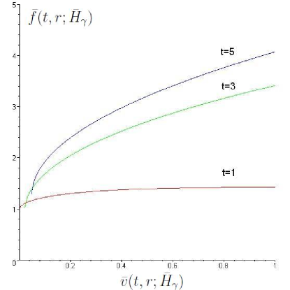
Figure 1. $\bar{f}(t,r;\bar{H}_{\gamma})$ as a function of $\bar{v}(t,r;\bar{H}_{\gamma})$ at fixed moment of time and different $\gamma$.

Let us compare the conditional expectation of the portfolio at a fixed value of factor for two strategies under consideration. We substitute (6.28) and (3.7) in the formula (6.26) for $\bar{f}(t,r)$ and after computations we get the following proposition.

Proposition 6.1.

For $\gamma=0,\theta=0$, $t>0$ the following inequality holds:

$$(\bar{f}(t,r;\bar{H}_{\gamma})-\bar{f}(t,r;H_{\theta}))|_{\gamma=0,\theta=0}=\frac{(\alpha_{1}-1)^{2}(r+\frac{B}{\beta})^{2}t(\frac{e^{-\beta t}-1}{t\beta}+1)^{2}}{2\sigma_{1}^{2}}>0.$$

Proposition 6.2.

There exists $t_{*}>0$ such that for all $t\in(0,t_{*})$ the following statement hold:

1. if $\alpha_{1}\neq 1$ and the factor satisfies the condition

   $$(r+\frac{B}{\beta})(r+\frac{A_{1}}{(\alpha_{1}-1)})>0,$$ (6.29)

   then there exists $\gamma_{*}>0$ such that for all $\gamma\in(0,\gamma_{*})$

   $$\bar{f}(t,r;\bar{H}_{\gamma})-\bar{f}(t,r;H_{\theta})>0;$$

2. if $\alpha_{1}=1$ and $A_{1}>0$, then $\bar{f}(t,r;\bar{H}_{\gamma})-\bar{f}(t,r;H_{\theta})>0$ for all $\gamma>0.$

Proof. We consider the difference $\bar{f}(t,r;\bar{H}_{\gamma})-\bar{f}(t,r;H_{\theta})$ as a function of $t$ at other parameters fixed. We denote this difference as $q(t)$. The computations show that $q^{\prime}(0)=0$ and

$$\begin{array}[]{rcl}q^{\prime\prime}(0)&=&(8r^{2}\gamma^{2}\lambda(\alpha_{1}-1)^{3}-2((1+2\gamma)\gamma\beta\sigma_{1}r^{2}+\\ &&+((1+2\gamma)\gamma B\sigma_{1}-8\gamma^{2}\lambda A_{1})r)(\alpha_{1}-1)^{2}-\\ &&-2\Big{(}(-2(2\gamma+1)\gamma^{2}\lambda\sigma_{1}^{2}+(1+2\gamma)\gamma A_{1}\beta\sigma_{1})r+\\ &&+(1+2\gamma)\gamma A_{1}B\sigma_{1}-4\gamma^{2}\lambda A_{1}^{2}\Big{)}(\alpha_{1}-1)+\\ &&+4(2\gamma+1)\gamma^{2}\lambda\sigma_{1}^{2}A_{1})(\sigma_{1}^{3}(1+6\gamma+12\gamma^{2}+8\gamma^{3}))^{-1}.\end{array}$$

The denominator of this expression is positive. One can see that if $\alpha_{1}=1$ and $A_{1}>0$, then $q^{\prime\prime}(0)>0$. This proves the second part of the proposition.

If $\alpha_{1}\neq 1$, than we expand the numerator $q^{\prime\prime}(0)=q^{\prime\prime}(0,\gamma)$ in series with respect to $\gamma$ about zero:

$$q^{\prime\prime}(0,\gamma)=-2\beta\sigma_{1}(\alpha_{1}-1)^{2}(r+\frac{B}{\beta})(r+\frac{A_{1}}{(\alpha_{1}-1)})\gamma+O(\gamma^{2}).$$

This expression is positive if the condition (6.29) holds. $\Box$

Fig.2 shows the graphs of conditional expectations for two strategies for the same parameters of model as in Fig.1. Here $4\gamma=\theta=0.1$. This example shows that our strategy for realistic values of parameter gives greater expectation of portfolio’s long-run expected growth rate till the moment $t^{*}$ and this situation can hold within several years.

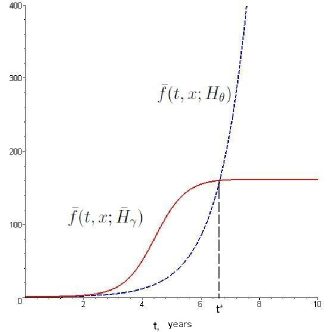
Figure 2. The conditional expectation of portfolio’s long-run expected growth rate $\bar{f}(t,r;h)$ for our strategy $\bar{H}_{\gamma}$ (solid line) and in the case of the strategy of Bielecki and Pliska $H_{\theta}$ (dashed line).

Taking into account the principle of constructing the function $\bar{Q}_{\gamma}(t,r;h)$ it makes sense to compare two strategies for $\gamma=\theta/4$ and small $\theta$. First we compare the results as $t\rightarrow\infty.$ At any fixed $x$ we get $\displaystyle\lim_{t\rightarrow\infty}\bar{H}_{\gamma}(t)=-\frac{1}{\alpha_{1}-1}$ in the case $\alpha_{1}\neq 1$ and $\displaystyle\lim_{t\rightarrow\infty}\bar{H}_{\gamma}(t)=\frac{A_{1}}{\sigma^{2}_{1}}$ in the case $\alpha_{1}=1.$ Thus, the limit $\bar{H}_{\gamma}(t)$ is discontinuous as a function of $\alpha_{1}$. We introduce the following denotation:

$$\bar{\rho}(\gamma):=\lim_{t\rightarrow\infty}\frac{\bar{Q}_{\gamma}(t,r;\bar{H}_{\gamma})}{t}.$$

Computations show that

$$\begin{array}[]{rcl}\bar{\rho}(\gamma)&=&\frac{A_{1}}{1-\alpha_{1}}-(\gamma+\frac{1}{2})\frac{\sigma_{1}^{2}}{(\alpha_{1}-1)^{2}},\quad\alpha_{1}\neq 1,\\ \bar{\rho}(\gamma)&=&\frac{A_{1}^{2}}{2\sigma_{1}^{2}}-\frac{B}{\beta},\quad\alpha_{1}=1.\end{array}$$

The value $\bar{\rho}(\gamma)$ corresponds to the expected rate of growth of capital at infinity, it is analogous to $\rho(\theta)$ in the model of Bielecki and Pliska, see(3.8). Fig.3 shows this function at the same values of parameter as at Fig.1, $\theta$ varies from $0$ to $1$, $\gamma=\frac{\theta}{4}.$

After the limit pass as $\theta\rightarrow 0$ we get from (3.9)

$$\lim_{\theta\rightarrow 0}\rho_{\theta}=-\frac{B}{\beta}+\frac{1}{2\sigma_{1}^{2}}(A_{1}-\frac{B}{\beta}(\alpha_{1}-1))^{2}-\frac{\lambda^{2}(\alpha_{1}-1)^{2}}{4\sigma^{2}\beta}.$$ (6.30)

If we set directly $\gamma=0$ in $\frac{\bar{Q}_{\gamma}(t,x;\bar{H}_{\gamma})}{t}$, and then perform the limit pass as $t\rightarrow\infty$, we get (6.30) without the last term, containing $\lambda$.

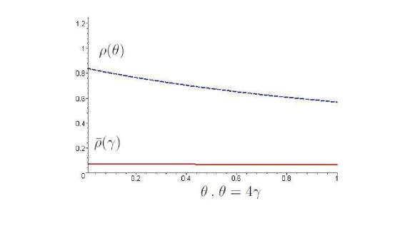
Figure 3. The expected rate of growth of capital at infinity: $\bar{\rho}(\gamma)$ for our strategy, $\rho(\theta)$ for the Bielecki and Pliska strategy, $\theta=4\gamma$.

6.3. Asymptotics of the proportions of capitals

In this section we study the asymptotics of proportions of the portfolio capital as times goes to infinity for the cases of two and three assets depending on one factor with uniform initial distribution. We recall that for the Gaussian initial distribution basically there arises a restriction on application of strategy for large $t$, therefore the computation of asymptotics is impossible.

For the case of two assets depending on one factor we have the system $\eqref{1FactorFCapital},$ $\eqref{1Factor}$ for $m=2$. The functions corresponding to the proportions of capital are found in Sec.6.1.2:

$$H_{1}(t)=-\frac{K_{1}}{2K_{2}},$$ (6.31)

$$H_{2}(t)=1+\frac{K_{1}}{2K_{2}}.$$ (6.32)

We denote the asymptotic limits of the proportions of capitals as follows:

$$H_{1(2)}^{\infty}:=\lim_{t\to\infty}(H_{1}(t)),\quad H_{2(2)}^{\infty}:=\lim_{t\to\infty}(H_{2}(t)).$$

The computation shows that the following proposition holds:

Proposition 6.3.

Let $H_{1}(t)$ and $H_{2}(t)$ be defined as $\eqref{H12}$, $\eqref{H22}$, then

1. if $\alpha_{1}\neq\alpha_{2}$, then $H_{1(2)}^{\infty}=\displaystyle-\frac{\alpha_{2}}{\alpha_{1}-\alpha_{2}},\quad H_{2(2)}^{\infty}=1-H_{1(2)}^{\infty};$

2. if $\alpha_{1}=\alpha_{2}$, then $H_{1(2)}^{\infty}=\mathcal{K}_{1}\cdot\infty,$

   $\mathcal{K}_{1}=\displaystyle\frac{\gamma\alpha_{1}((\sigma_{11}-\sigma_{12})\lambda_{1}+(\sigma_{21}-\sigma_{22})\lambda_{2}+(\sigma_{31}-\sigma_{32})\lambda_{3})}{(\sigma_{11}^{2}+\sigma_{12}^{2}+\sigma_{13}^{2}+\sigma_{21}^{2}+\sigma_{22}^{2}+\sigma_{23}^{2})(2\beta\gamma-1)};$

3. if $\mathcal{K}_{1}=0$, then $H_{1}(t)\equiv H_{1(2)}^{\infty}=\displaystyle\frac{(2\beta\gamma-1)\sigma_{2}^{2}+A_{2}-A_{1}}{(\sigma_{1}^{2}+\sigma_{2}^{2})(2\beta\gamma-1)}.$

Thus, the limit values of proportions at infinity in the case of two assets depends only on parameters $\alpha_{1}$ and $\alpha_{2}$, if $\alpha_{1}\neq\alpha_{2}$. In the case $\alpha_{1}=\alpha_{2}$ the limit value depends on other parameters, too. For large $t$ it worth to invest to an asset that is less depending on the factor (the respective $\alpha_{i}$ is the smallest my modulus), despite of trends and volatilies.

In the case of three assets depending on one factor ($m=3,$ $n=1$) the proportions of the capital can be also found according to Sec.4. Let us introduce the denotation of limits of proportions of the capital $H_{i}(t),i=1,2,3$ as the time tends to infinity:

$$H_{1(3)}^{\infty}:=\lim_{t\to\infty}(H_{1}(t)),H_{2(3)}^{\infty}:=\lim_{t\to\infty}(H_{2}(t)),H_{3(3)}^{\infty}:=\lim_{t\to\infty}(H_{3}(t)).$$

The explicit formulas for asymptotic limits are the following:

$$H_{1(3)}^{\infty}=(2\beta(U_{3}(\alpha_{2}^{2}-\alpha_{1}\alpha_{2})+U_{2}(\alpha_{3}^{2}-\alpha_{1}\alpha_{3}))\gamma+(-A_{1}+A_{3}-U_{3})\alpha_{2}^{2}+$$

$$+(-A_{1}+A_{2}-U_{2})\alpha_{3}^{2}+(2A_{1}-A_{2}-A_{3})\alpha_{2}\alpha_{3}+(A_{2}-A_{3}+U_{3})\alpha_{1}\alpha_{2}+(-A_{2}+A_{3}+U_{2})\alpha_{1}\alpha_{3})/$$

$$(2\beta((U_{2}+U_{3})\alpha_{1}^{2}+(U_{1}+U_{3})\alpha_{2}^{2}+(U_{1}+U_{2})\alpha_{3}^{2})+4\beta(-U_{3}\alpha_{1}\alpha_{2}-U_{2}\alpha_{1}\alpha_{3}-U_{1}\alpha_{2}\alpha_{3}))\gamma+$$

$$+(-U_{2}-U_{3})\alpha_{1}^{2}+(-U_{1}-U_{3})\alpha_{2}^{2}+(-U_{1}-U_{2})\alpha_{3}^{2}+2(U_{3}\alpha_{1}\alpha_{2}+U_{2}\alpha_{1}\alpha_{3}+U_{1}\alpha_{2}\alpha_{3})),$$

$$H_{2(3)}^{\infty}=(2\beta(U_{3}(\alpha_{1}^{2}-\alpha_{1}\alpha_{2})+U_{1}(\alpha_{3}^{2}-\alpha_{2}\alpha_{3}))\gamma+(-A_{2}+A_{3}-U_{3})\alpha_{1}^{2}+$$

$$+(A_{1}-A_{2}-U_{1})\alpha_{3}^{2}+(-A_{1}+2A_{2}-A_{3})\alpha_{1}\alpha_{3}+(A_{1}-A_{3}+U_{3})\alpha_{1}\alpha_{2}+(-A_{1}+A_{3}+U_{1})\alpha_{2}\alpha_{3})/$$

$$(2\beta((U_{2}+U_{3})\alpha_{1}^{2}+(U_{1}+U_{2})\alpha_{2}^{2}+(U_{1}+U_{2})\alpha_{3}^{2})+4\beta(-U_{3}\alpha_{1}\alpha_{2}-U_{2}\alpha_{1}\alpha_{3}-U_{1}\alpha_{2}\alpha_{3}))\gamma+$$

$$+(-U_{2}-U_{3})\alpha_{1}^{2}+(-U_{1}-U_{3})\alpha_{2}^{2}+(-U_{1}-U_{2})\alpha_{3}^{2}+2(U_{3}\alpha_{1}\alpha_{2}+U_{2}\alpha_{1}\alpha_{3}+U_{1}\alpha_{2}\alpha_{3})),$$

$$H_{3(3)}^{\infty}=(2\beta(U_{2}(\alpha_{1}^{2}-\alpha_{1}\alpha_{3})+U_{1}(\alpha_{2}^{2}-\alpha_{2}\alpha_{3}))\gamma+(A_{2}-A_{3}-U_{2})\alpha_{1}^{2}+$$

$$+(A_{1}-A_{3}-U_{1})\alpha_{2}^{2}+(-A_{1}-A_{2}+2A_{3})\alpha_{1}\alpha_{2}+(A_{1}-A_{2}+U_{2})\alpha_{1}\alpha_{3}+(-A_{1}+A_{2}+U_{1})\alpha_{2}\alpha_{3})/$$

$$(2\beta((U_{2}+U_{3})\alpha_{1}^{2}+(U_{1}+U_{2})\alpha_{2}^{2}+(U_{1}+U_{2})\alpha_{3}^{2})+4\beta(-U_{3}\alpha_{1}\alpha_{2}-U_{2}\alpha_{1}\alpha_{3}-U_{1}\alpha_{2}\alpha_{3}))\gamma+$$

$$+(-U_{2}-U_{3})\alpha_{1}^{2}+(-U_{1}-U_{3})\alpha_{2}^{2}+(-U_{1}-U_{2})\alpha_{3}^{2}+2(U_{3}\alpha_{1}\alpha_{2}+U_{2}\alpha_{1}\alpha_{3}+U_{1}\alpha_{2}\alpha_{3})),$$

where

$$U_{1}=\sigma_{11}^{2}+\sigma_{12}^{2}+\sigma_{13}^{2}+\sigma_{14}^{2},$$

$$U_{2}=\sigma_{21}^{2}+\sigma_{22}^{2}+\sigma_{23}^{2}+\sigma_{24}^{2},$$

$$U_{3}=\sigma_{31}^{2}+\sigma_{32}^{2}+\sigma_{33}^{2}+\sigma_{34}^{2}.$$

Let us note that the limit behavior depends in general case on all parameters of the model and this difference from the case of two assets seems strange. Nevertheless, if parameters $\alpha_{i}$ for a pair of assets coincide, then the situation is analogous to the case of two assets. For example, if $\alpha_{2}=\alpha_{3}$, then for any values of other parameters $H_{1(3)}^{\infty}=\displaystyle\frac{\alpha_{2}}{\alpha_{2}-\alpha_{1}}$. Moreover, $H_{2(3)}^{\infty}$ and $H_{3(3)}^{\infty}$ depend on other parameters of the model, too. The case where all $\alpha_{i}$ are equal, is degenerate, as above:

$$H_{1(3)}^{\infty}=\mathcal{K}_{1}\cdot\infty,\quad\mathcal{K}_{1}=\displaystyle\frac{\gamma\alpha_{1}(\sum_{l=1}^{4}\lambda_{l}\sum_{i,j,k}(-1)^{i+j-1}\sigma_{k}^{2}(\sigma_{il}-\sigma_{jl})}{(2\beta\gamma-1)\sum_{i\neq j,i,j=1}^{3}\sigma^{2}_{i}\sigma_{j}^{2})},$$

where $\displaystyle\sigma_{i}^{2}=\sum_{k=1}^{4}\sigma^{2}_{ik},\,i=1,2,3,$ where $i,j,k$ are all even combinations of indices $(1,2,3)$. If $\mathcal{K}_{1}=0$, then

$$H_{1}(t)\equiv H_{1(3)}^{\infty}=\displaystyle\frac{(2\beta\gamma-1)\sigma_{2}^{2}\sigma_{3}^{2}+(A_{2}-A_{1})\sigma_{3}^{2}+(A_{3}-A_{1})\sigma_{2}^{2}}{(2\beta\gamma-1)\sum_{i\neq j,i,j=1}^{3}\sigma^{2}_{i}\sigma_{j}^{2}}.$$

6.4. Influence of different parameters of model on the optimal strategy of investment for small time

It is interesting to note that for small time the strategy of investment depends on all parameters and differs significantly on the limit behavior as $t\to\infty$. We show the results of computations for the case of two and three assets (the values of parameters are given in the tables 1 and 2, respectively).

As we have seen for the case of two assets ($n=2$) the limit behavior of the proportions depends only on parameters $\alpha_{1},\alpha_{2}$. For small times the strategy is different:

• Fig. 4 presents graphs for the proportions of capital for different $\beta$. For greater $\beta$ the function reaches its asymptotical value quicker;

• Fig. 5 presents graphs for the proportions of capital in dependence on parameter $\sigma_{11}$. For small $t$ an increasing of $\sigma_{11}$ results to a decreasing of the proportion of corresponding asset in the portfolio;

• Parameter $A_{1}$ influences very weakly at large times, nevertheless, for small $t$ its influence is significant (see Fig. 6).

To study the strategy of optimal investment in the case of three assets ($n=3$), we analyze functions $H_{i}(t),i=1,2,3,$ changing the values of parameters $\beta,\sigma_{ij},A_{i},$ $i=1,2,3;j=1,2,3,4$:

• First we set the parameters $\alpha_{i}$ very close and study the influence of $\beta$, $\beta<0$, other parameters are fixed. Fig.7 illustrates the dependence of $H_{i}(t)$ n $\beta$.

• Then we fix the parameter $\beta$ ($\beta=-2$) and change $\sigma_{11}$, the volatility of the first asset, other parameters are as in Fig.7. Fig.8 the dependence of $H_{i}(t)$ on $\sigma_{11}$. Since

  $$H_{1(3)}^{\infty}=\lim_{t\to\infty}H_{1}(t)=\frac{\Psi_{1}}{\Psi_{2}\sigma_{11}^{2}+\Psi_{3}},$$

  where $\Psi_{1},\Psi_{2},\Psi_{3}$ do not depend of $\sigma_{11}$, if $\sigma_{11}$ increases, then the limit value $H_{1}(t)$ becomes smaller. Thus, the asset with a small volotility is preferable.

• Then we fixe $\beta$ and $\sigma_{11}$ and study the influence of $A_{1}$. First of all we group the expression $H_{1(3)}^{\infty}$ with respect to $A_{1}$ and get

  $$H_{1(3)}^{\infty}=\frac{(\alpha_{2}-\alpha_{3})^{2}A_{1}}{\Phi_{1}}+\Phi_{2},$$

  where $\Phi_{1},\Phi_{2}$ do not depend of $A_{1}$. Thus, the parameter $A_{i}$ influences on the strategy for small $t$, whereas for large $t$ this dependence is very weak provided $\alpha_{i}$ are close (see Fig.9).

• The influence of an increasing of the risk parameter $\gamma$ analogous to an increasing of $\beta$ by modulus.

Let us summarize the influence of parameters on the character of the optimal strategy, analogous in the case of two and three assets:

1. an increasing of parameters $\beta$ and $\gamma$ (by modulus) results a quicker attainment of the limit value as $t\to\infty$;

2. for small time a decreasing of volatility of $i$-th asset (the values of $\sigma_{ik}$) results an increasing of the proportion of this asset in the portfolio;

3. despite the fact that the trend $A_{i}$ does not influence on the limit behavior as $t\to\infty$, for small time the influence of this parameter if significant (increasing of $A_{i}$ results the increasing of proportion of the corresponding asset).

Remark 6.2.

Let us note that for our strategy any moment of time can be taken as the initial one. Therefore, we can reasonably find the moment of time $T$ for actualization of parameters of the model, i.e. for setting the time to zero. For every set of parameters of the model there exists its own ”infinity”, that is the time of achievement of the asymptotical value. For real data this time has an order of several years. It is natural to take this time as a time $\,T$ for actualization. As it follows from our considerations, if the risk parameter $\gamma$ increases, then $T$ becomes smaller, therefore, we have to actualize the model more frequently.

Table 1. Values of parameters for the case of two assets

	Fig.4	Fig.5	Fig.6
$\beta$	-1;-5	-1	-1
$\alpha_{1}$	0.5	0.5	0.5
$\alpha_{2}$	0.1	0.1	0.1
$\gamma$	1	1	1
$A_{1}$	0.1	0.1	0.1;0.5
$A_{2}$	0.1	0.1	0.1
$B$	1	1	1
$\sigma_{11}$	0.1	0.1;0.5	0.1
$\sigma_{21}$	0.1	0.1	0.1
$\sigma_{12}$	0.1	0.1	0.1
$\sigma_{22}$	0.1	0.1	0.1
$\sigma_{13}$	0.1	0.1	0.1
$\sigma_{23}$	0.1	0.1	0.1
$\lambda_{1}$	0.1	0.1	0.1
$\lambda_{2}$	0.1	0.1	0.1
$\lambda_{3}$	0.1	0.1	0.1

Table 2. Values of parameters for the case of three assets

	Fig.7	Fig.8	Fig.9
$\beta$	-0.9;-2;-5	-2	-2
$\alpha_{1}$	0.13	0.13	0.13
$\alpha_{2}$	0.12	0.12	0.12
$\alpha_{3}$	0.11	0.11	0.11
$\gamma$	1	1	1
$A_{1}$	0.1	0.1	0.5;2;5
$A_{2}$	0.1	0.1	0.1
$A_{3}$	0.1	0.1	0.1
$B$	1	1	1
$\sigma_{11}$	0.1	0.3;1.5;3	0.3
$\sigma_{21}$	0.1	0.1	0.1
$\sigma_{31}$	0.1	0.1	0.1
$\sigma_{12},\sigma_{22},\sigma_{32}$	0.1	0.1	0.1
$\sigma_{13},\sigma_{23},\sigma_{33}$	0.1	0.1	0.1
$\lambda_{1},\lambda_{2},\lambda_{3},\lambda_{4}$	0.1	0.1	0.1

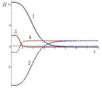
Figure 4. Influence of parameter $\beta$ on the strategy $H=(H_{1},H_{2})$: 1. $H_{1},$ for $\beta=-1$;   2. $H_{2},$ for $\beta=-1$;   3. $H_{1},$ for $\beta=-5$;   4. $H_{2},$ for $\beta=-5$.

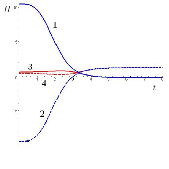
Figure 5. Influence of parameter $\sigma_{11}$ on the strategy $H=(H_{1},H_{2})$: 1. $H_{1},$ for $\sigma_{11}=0.1$;   2. $H_{2},$ for $\sigma_{11}=0.1$;   3. $H_{1},$ for $\sigma_{11}=0.5$;   4. $H_{2},$ for $\sigma_{11}=0.5$.

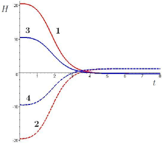
Figure 6. Influence of parameter $A_{1}$ on the strategy $H=(H_{1},H_{2})$: 1. $H_{1},$ for $A_{1}=0.1$;   2. $H_{2},$ for $A_{1}=0.1$;   3. $H_{1},$ for $A_{1}=0.5$;   4. $H_{2},$ for $A_{1}=0.5$.

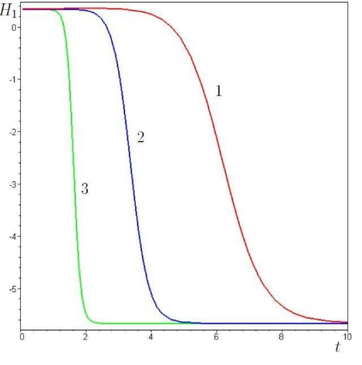
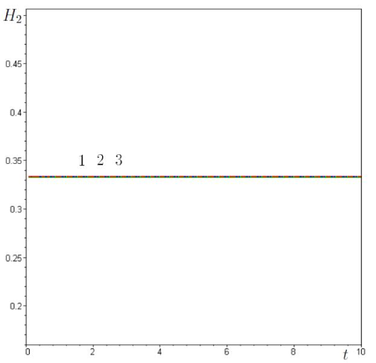
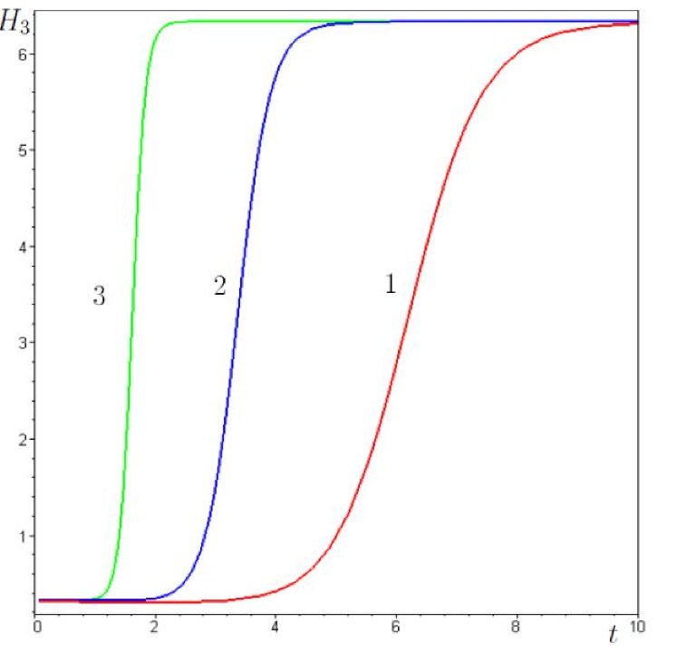
Figure 7. Influence of parameter $\beta$ on the strategy $\qquad(H_{1},H_{2},H_{3})$: 1. $\beta=-0.9$;   2. $\beta=-2$;   3. $\beta=-5$.

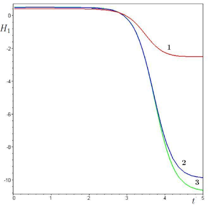
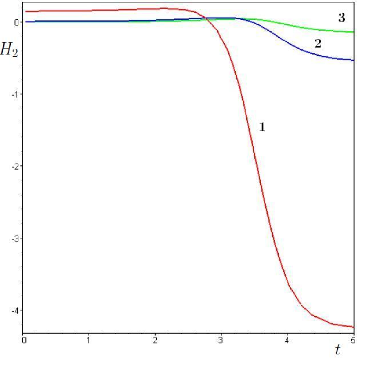
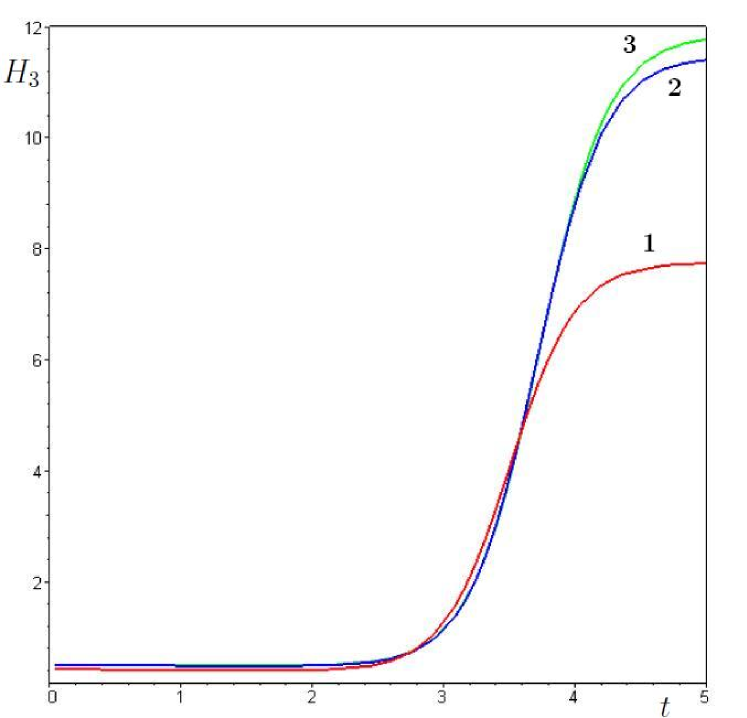
Figure 8. Influence of parameter $\sigma_{11}$ on the strategy $(H_{1},H_{2},H_{3})$: 1. $\sigma_{11}=0.3$;   2. $\sigma_{11}=1.5$;   3. $\sigma_{11}=3$.

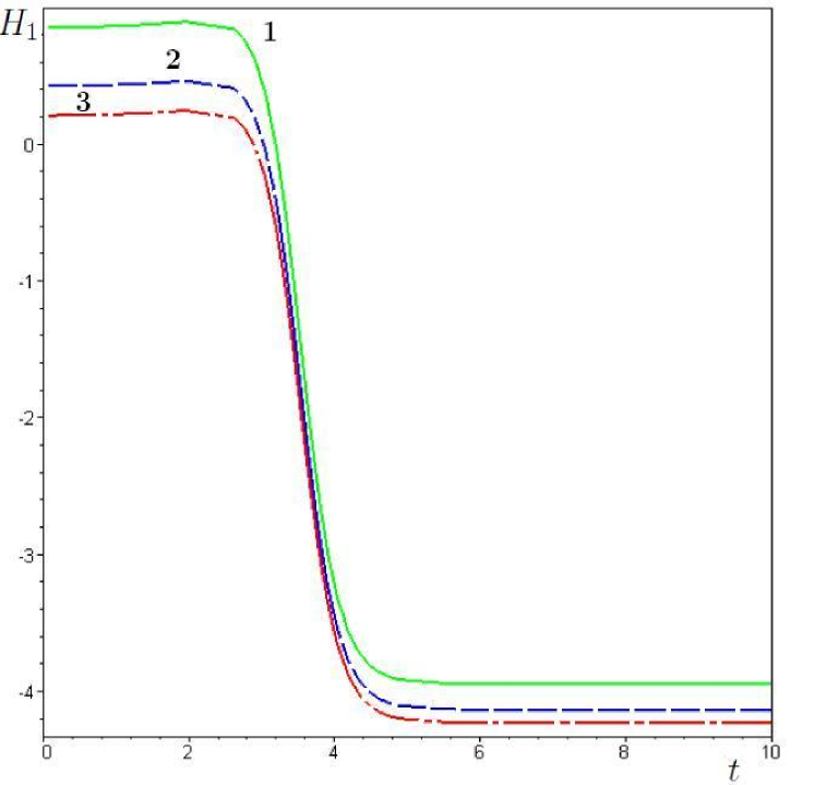
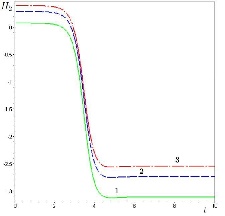
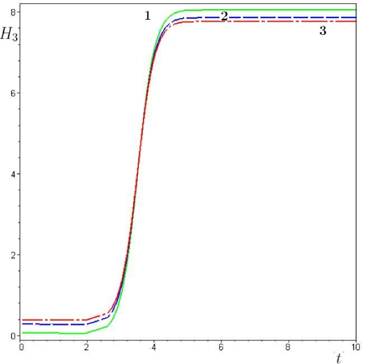
Figure 9. Influence of parameter $A_{1}$ on the strategy $(H_{1},H_{2},H_{3})$: 1. $A_{1}=5$;   2. $A_{1}=2$;   3. $A_{1}=0.5$.

7. A nonlinear interest rate (the Cox-Ingersoll-Ross model)

7.1. An auxiliary problem: the conditional expectation and variance

The strict theory by Bielecki and Pliska is restricted to the case of the factor with a constant volatility. The reason is that for this model the Hamilton-Jacobi-Bellman is reduced to a very special parabolic second order PDE where a sum of the order of derivatives and the order of polynomial in the coefficients at these derivatives is equal to two. In this section we consider another model of the interest rate where the volatility is proportional to the square root of the rate itself. The solution to problem can be found in this case for a special initial distribution of the interest rate.

We consider a particular case of system (4.1):

$$dF=(A+\alpha R)dt+\sigma dW_{1},$$ (7.1)

$$dR=(B+\beta R)dt+\lambda\sqrt{R}dW_{2}.$$ (7.2)

Here $B>0,\beta<0,\sigma>0,\lambda>0,A,\alpha$ are constants.

The first equation describes the return $F$ of asset with the trend that linearly depends on the interest rate $R,$ that obeys the Cox-Ingersoll-Ross model [10]. The inequality $-2\beta B>\lambda^{2}$ implies a positivity of the random process describing the interest rate [15]. The interest rate of the form (7.2) as a factor was considered, in particular, in the work [6], a step toward to the finding the optimal strategy in the sense of Bielecki-Pliska [4]. Nevertheless the authors obtain only partial results.

Let us assume that initially the interest rate $R$ is distributed uniformly on the interval $(0,L),L>0.$

Remark 7.1.

For the Vasicek model we obtain explicit formulae for initial Gaussian distribution including limiting cases. Nevertheless, for the Cox-Ingersoll-Ross we can get an explicit formula only for uniform initial distribution.

The Fokker-Planck equation for the join distribution of random values $F$ and $R$ given by system (7.1), (7.2), is

$$\begin{array}[]{rcl}&&\displaystyle\frac{\partial P(t,f,r)}{\partial t}+(A+\alpha r)\frac{\partial P(t,f,r)}{\partial f}+\beta P(t,f,r)+\\ &&\displaystyle+(B+\beta r-\lambda^{2})\frac{\partial P(t,f,r)}{\partial r}-\displaystyle\frac{1}{2}\sigma^{2}\frac{\partial^{2}P(t,f,r)}{\partial f^{2}}-\frac{1}{2}\lambda^{2}r\frac{\partial^{2}P(t,f,r)}{\partial r^{2}}=0,\end{array}$$ (7.3)

subject to initial conditions

$$P\left(0,f,r\right)=\delta\left(f-f_{0}\right){\chi_{(0,L)}(r)}.$$ (7.4)

Rigourously speaking, to define a probability density function $P\left(0,f,r\right)$ we have to divide the expression (7.4) by $L$. Nevertheless, as follows from the linearity of equation (7.3) and definitions (4.17), (4.18) this multiplier does no influence on the result of computations.

The Fourier transform with respect to $(f,r),$ the function $\hat{P}\left(t,\mu,\xi\right),$ obeys the equation

$$\begin{array}[]{rcl}\displaystyle{\frac{\partial}{\partial t}}\hat{P}\left(t,\mu,\xi\right)-\left(\alpha\,\mu+\beta\,\xi-i\frac{1}{2}{\lambda}^{2}{\xi}^{2}\right){\frac{\partial}{\partial{\xi}}}\hat{P}\left(t,\mu,\xi\right)+\\ +\displaystyle\left(\frac{1}{2}\,{\sigma}^{2}{\mu}^{2}+A\mu i+B\xi i\right)\hat{P}\left(t,\mu,\xi\right)=0,\end{array}$$ (7.5)

with initial conditions

$$\hat{P}(0,\mu,\xi)=\frac{1}{2\pi}\,e^{-i\mu\,f_{0}}\,\frac{e^{-i\xi L}-1}{i\xi}\rightarrow\frac{1}{2\pi}\,e^{-i\mu\,f_{0}}\,\delta(\xi)\,\mbox{\quad as \quad}\,L\to\infty.$$ (7.6)

Equation (7.5) has the first order and can be integrated. The solution to the problem (7.5),(7.6) in the limit case $L\to\infty$ can be found by a standard way:

$$\hat{P}(t,\mu,\xi)={e^{-{\frac{2\,if_{0}\mu\,\lambda^{2}+2\,t\,A\mu\,{\lambda}^{2}\,i+2\,t\,B\,{\beta}+t\,{\sigma}^{2}{\mu}^{2}{{\lambda}}^{2}}{2\,{{\lambda}}^{2}}}}}{\delta}\left(s(t,\mu,\xi)\right)\times$$

$$\times\left(\frac{{{\lambda}}^{2}(2\,i{\alpha}\,\mu+2\,i{\beta}\,{\xi}+{{\lambda}}^{2}{{\xi}}^{2})\cosh\left(\frac{t\sqrt{2\,i{\alpha}\,\mu\,{{\lambda}}^{2}+{{\beta}}^{2}}}{2}+i\arctan({\frac{{{\lambda}}^{2}{\xi}+i{\beta}}{\sqrt{2\,i{\alpha}\,\mu\,{{\lambda}}^{2}+{{\beta}}^{2}}}})\right)^{2}}{2\,i{\alpha}\,\mu\,{{\lambda}}^{2}+{{\beta}}^{2}}\right)^{-{\frac{B}{{{\lambda}}^{2}}}},$$

where

$$\begin{array}[]{rcl}s(t,\mu,\xi)=-{\frac{\left(\left({\beta}-\sqrt{2\,i{\alpha}\,\mu\,{{\lambda}}^{2}+{{\beta}}^{2}}\right){\xi}+2\,{\alpha}\,\mu\right){e^{-t\sqrt{2\,i{\alpha}\,\mu\,{{\lambda}}^{2}+{{\beta}}^{2}}}}+\left(-{\beta}-\sqrt{2\,i{\alpha}\,\mu\,{{\lambda}}^{2}+{{\beta}}^{2}}\right){\xi}-2\,{\alpha}\,\mu}{\sqrt{2\,i{\alpha}\,\mu\,{{\lambda}}^{2}+{{\beta}}^{2}}+i{{\lambda}}^{2}{\xi}-{\beta}+\left(\sqrt{2\,i{\alpha}\,\mu\,{{\lambda}}^{2}+{{\beta}}^{2}}-i{{\lambda}}^{2}{\xi}+{\beta}\right){e^{-t\sqrt{2\,i{\alpha}\,\mu\,{{\lambda}}^{2}+{{\beta}}^{2}}}}}}.\end{array}$$

We apply (4.17) and (4.18):

$$\hat{P}(t,0,\xi)=\theta(t,\xi){\delta}\left(s(t,0,\xi)\right),$$ (7.7)

$$\partial_{\mu}\hat{P}(t,0,\xi)=\phi(t,\xi)\,\delta(s(t,0,\xi))+\psi(t,\xi)\,\delta^{\prime}_{\mu}(s(t,0,\xi)),$$ (7.8)

$$\partial^{2}_{\mu}\hat{P}(t,0,\xi)=q_{1}(t,\xi)\,\delta(s(t,0,\xi))+q_{2}(t,\xi)\,\delta^{\prime}_{\mu}(s(t,0,\xi))+q_{3}(t,\xi)\delta^{\prime\prime}_{\mu}(s(t,0,\xi)),$$ (7.9)

where

$$s(t,0,\xi)=\frac{2\beta\xi}{i\xi\lambda^{2}+(2\beta-i\xi\lambda^{2})e^{-\beta t}},$$

$$\theta(t,\xi)=\left(\frac{-i\lambda^{2}(i\xi^{2}\lambda^{2}-2\beta\xi)\cosh\left(\frac{\beta t}{2}+i\arctan(\frac{\lambda^{2}\xi+i\beta}{\beta})\right)^{2}e^{\beta t}}{\beta^{2}}\right)^{\frac{-B}{\lambda^{2}}},$$

$$\phi(t,\xi)=\theta(t,\xi)\left(L_{1}-i(At+f_{0})\right),\quad\psi(t,\xi)=\theta(t,\xi)L_{2},$$

$$L_{1}=\frac{B\alpha\left((4\beta\lambda^{4}\xi^{2}-i\lambda^{6}\xi^{3}+4i\beta^{2}\lambda^{2}\xi)t+(4\beta^{2}-2\lambda^{4}\xi^{2}-6i\beta\lambda^{2}\xi)\right)}{\beta\lambda^{2}\xi(\lambda^{2}\xi+2i\beta)^{2}}\times$$

$$\times\frac{\sinh\left(\frac{\beta t}{2}+i\arctan(\frac{\lambda^{2}\xi+i\beta}{\beta})\right)}{\cosh\left(\frac{\beta t}{2}+i\arctan(\frac{\lambda^{2}\xi+i\beta}{\beta})\right)}+\frac{2\alpha B(i\lambda^{2}\xi(\lambda^{4}\xi^{2}-5\beta^{2})-4\beta\lambda^{4}\xi^{2})+2\beta^{3}}{\beta^{2}\lambda^{2}\xi(\lambda^{2}\xi+2i\beta)^{2}},$$

$$L_{2}=\frac{-\alpha\xi^{2}\lambda^{4}e^{2\beta t}+2((\lambda^{2}\xi+2i\beta)\lambda^{2}\xi t-2i\lambda^{2}\xi+2\beta)\alpha\beta e^{\beta t}+4i\alpha\beta\lambda^{2}\xi+\alpha\lambda^{2}\xi-4\alpha\beta^{2}}{i\beta\lambda^{2}\xi(e^{\beta t}-1)+2\beta^{2}}.$$

We do not write here the explicit values of $q_{i}(t,\xi),i=1,2,3$, since they are very long.

We substitute (7.7),(7.8),(7.9) in (4.17) and (4.18) and after cumbersome but standard computations get

$$\begin{array}[]{rcl}&&\bar{f}(t,r)=\displaystyle f_{0}+\left(A-\frac{\alpha}{\beta}\right)t+\frac{(1-e^{\beta t})\alpha r}{\beta}-{\frac{\left(2+{\lambda}^{2}\right)\alpha\,e^{2\beta\,t}}{{\beta}^{2}}}+\\ &&+\left({\frac{\left(1+{\lambda}^{2}\right)\alpha\,t}{\beta}}+{\frac{\left(2+{\lambda}^{2}\right)\alpha}{{\beta}^{2}}}\right){e^{\beta\,t}},\end{array}$$ (7.10)

$$\begin{array}[]{rcl}&&\bar{v}(t,r)=\displaystyle t\sigma^{2}+\left(-\frac{2e^{3\beta t}}{\beta^{3}}+\frac{(2\beta t+3)e^{2\beta t}}{\beta^{3}}-\frac{2e^{\beta t}}{\beta^{3}}+\frac{1}{\beta^{3}}\right)\alpha^{2}\lambda^{2}r+\\ &&\displaystyle+\left({4e^{4\beta t}}-\frac{3(4\beta t+5)e^{3\beta t}}{2}+(\beta^{2}t^{2}+4\beta t+6)e^{2\beta t}+\frac{(2\beta^{2}t^{2}-2\beta t-5)e^{\beta t}}{2}\right)\frac{\alpha^{2}\lambda^{4}}{\beta^{4}}+\\ &&\displaystyle+\left(\frac{5Be^{4\beta t}}{2}-{2B(\beta t+3)e^{3\beta t}}+\frac{15Be^{2\beta t}}{2}-{4Be^{\beta t}}-{B{\beta}t}\right)\frac{\alpha^{2}\lambda^{2}}{\beta^{4}}.\end{array}$$ (7.11)

7.2. Example of portfolio consisting of two assets

We consider a simple asset allocation example, featuring an interest rate which affects a stock index and also serves as a second investment opportunity, illustrates how factors which are commonly used for forecasting returns can be explicitly incorporated in a portfolio optimization model. This example was systematically considered in the works by T.Bielecki and S.Pliska (see [4], [5], [6]). The dynamics of the security prices is

$$\frac{dS_{1}(t)}{S_{1}(t)}=(A_{1}+\alpha_{1}R(t))dt+\sigma_{1}dW_{1}(t),$$

$$\frac{dS_{2}(t)}{S_{2}(t)}=R(t)dt,$$

where $R(t)$ is the Cox-Ingersoll-Ross interest rate (7.2).

The capital of portfolio obeys the equation $\displaystyle\frac{dV}{V}=h\frac{dS_{1}}{S_{1}}+(1-h)\frac{dS_{2}}{S_{2}}$, where the scalar valued function $h$ is interpreted as the proportion of capital invested in the risky asset, leaving the proportion $1-h$ invested in the bank account.

Remark 7.2.

We can consider a portfolio consisting of any number of assets, as it was done for the case of the Vasicek-type interest rate.

Let us denote $\ln V=F$. Then

$${dF}=\left(A_{1}h-\frac{1}{2}\sigma_{1}^{2}h^{2}+\Big{(}(h-1)\,\alpha_{1}+1\Big{)}\,R\right)dt+\sigma_{1}hdW_{1}.$$ (7.12)

For the system (7.12), (7.2) we apply the formulae for conditional mathematical expectation and variance (LABEL:nonlinFurCME), (LABEL:nonlinFurCVar) after substitution

$$A=A_{1}h-\frac{1}{2}\sigma_{1}^{2}h^{2},\quad\alpha=(\alpha_{1}-1)h+1,\quad\sigma=\sigma_{1}h.$$ (7.13)

We consider again the functional (5.2):

$$\bar{Q}_{\gamma}(t,r;h)=\bar{f}(t,r;h)-\gamma\bar{v}(t,r;h),$$

where $\gamma$ is the risk aversion coefficient, and find the optimal strategy in the sense of Definition 5.1.

According to (LABEL:nonlinFurCME), (LABEL:nonlinFurCVar) and (7.13) we get

$$\bar{Q}_{\gamma}(t,r;h)=K_{2}h^{2}+K_{1}h+K_{0},$$

where $K_{i}$ and smooth functions of $t,r$ and coefficients $A_{1},\alpha_{1},\sigma_{1},B,\beta,\lambda,\gamma$. These functions can be expressed through elementary functions, nevertheless, these expressions are cumbersome and we do not write them. Since $\bar{Q}_{\gamma}(t,r;h)$ is quadratic with respect $h$, and

$$K_{2}=-\frac{t\sigma_{1}^{2}h^{2}}{2}-\gamma\bar{v}(t,r;h)|_{(\alpha=\alpha_{1}-1,\,\sigma=\sigma_{1})}<0,$$

then $\bar{Q}_{\gamma}(t,r;h)$ has a unique point of maximum (analogous to the linear case, see Sec.6), the respective optimal strategy in the sense of definition 5.1 is the following:

$$\bar{H}_{\gamma}=\frac{-K_{1}}{2K_{2}}=$$

$$=\frac{(1-\alpha_{1})(M_{4}e^{4\beta t}+M_{3}e^{3\beta t}+M_{2}e^{2\beta t}+M_{1}e^{\beta t}+M_{0})+A_{1}\beta^{4}t}{(1-\alpha_{1})^{2}(M_{4}e^{4\beta t}+M_{3}e^{3\beta t}+N_{2}e^{2\beta t}+N_{1}e^{\beta t}+N_{0})+(2\gamma+1)\sigma_{1}^{2}\beta^{4}t},$$

where

$$M_{4}=\gamma\lambda^{2}(8\lambda^{2}+5B),\quad M_{3}=-\gamma\lambda^{2}\left((3\lambda^{2}+B)4\beta t+15\lambda^{2}+4r\beta+12B\right),$$

$$M_{2}=2\gamma\lambda^{4}\beta^{2}t^{2}+(2\lambda^{2}+\beta r)4\gamma\beta\lambda^{2}t+12\gamma\lambda^{4}+(5B+2\beta r)3\gamma\lambda^{2}-(\lambda^{2}+B)\beta^{2},$$

$$M_{1}=2\gamma\lambda^{4}\beta^{2}t^{2}+(\beta^{2}-2\gamma\lambda^{2})\beta\lambda^{2}t-5\gamma\lambda^{4}+(\beta^{2}-4\gamma\beta r-8\gamma B)\lambda^{2}+\beta^{3}r+\beta^{2}B,$$

$$M_{0}=(\beta^{2}-2\gamma\lambda^{2})\beta Bt+2\gamma\lambda^{2}\beta r-\beta^{3}r,\quad N_{1}=\gamma\lambda^{2}(2\beta^{2}\lambda^{2}t^{2}-2\beta\lambda^{2}t-5\lambda^{2}-4\beta r-8B),$$

$$N_{2}=\gamma\lambda^{2}(2\lambda^{2}\beta^{2}t^{2}+(2\lambda^{2}+\beta r)4\beta t+12\lambda^{2}+6\beta r+15B),\quad N_{0}=2\gamma\beta\lambda^{2}(-Bt+r).$$

We get

$$\lim_{t\rightarrow\infty}\bar{H}_{\gamma}=\lim_{t\rightarrow\infty}\bar{H}_{\gamma}(t)=\frac{(\alpha_{1}-1)(\beta^{2}B-2\gamma\lambda^{2}B)-A_{1}\beta^{3}}{(\alpha_{1}-1)^{2}2\gamma\lambda^{2}B+(2\gamma+1)\sigma_{1}^{2}\beta^{3}}.$$ (7.14)

As was shown in Sec.6, in the case of a linear interest rate model

$$\lim_{t\rightarrow\infty}\bar{H}_{\gamma}(t)=\frac{-1}{\alpha_{1}-1},\quad\alpha_{1}\neq 1.$$

This expression can be obtained by a limit pass in (7.14) as $\gamma\rightarrow\infty$ and $\sigma_{1}\rightarrow 0$.

8. Comparing the optimal strategies for linear and nonlinear models of the interest rate

We set the inferest rate $r=0.05,$ the initial capital of portfolio $f_{0}=0.08,$ the risk aversion coefficient $\gamma=0.1,$ the parameters $B=0.05,$ $\beta=-1,$ $\lambda=0.04,$ $A_{1}=0.15,$ $\alpha_{1}=-1,$ $\sigma_{1}=0.2$ are taken from [5].

Fig. 10 illustrates the corresponding optimal strategies of investment for the case of linear (solid line) and nonlinear (dashed line) interest rate for their uniform initial distribution. We see that these strategies are very different. To approach the optimal strategy for the nonlinear case to the strategy for the linear case we should choose A larger risk sensitive parameter $\gamma$.

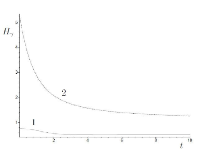
Figure 10. Comparing the optimal strategies for different models of the interest rate: 1. Vasicek-type interest rate   2. Cox-Ingersoll-Ross interest rate.

As we have seen, in the case of the Vasicek-type interest rate the asset less dependent on the factor is preferable for the investment for a large time. As follows from different combination of parameters, for the Cox-Ingersoll-Ross interest rate the properties of the factor are taken into account more effectively.

Remark 8.1.

If we assume additionally that the variance of the return of the risky asset satisfying (7.1) is proportional to the interest rate, we fall in the situation of the Heston model [19], one of the most popular models of stochastic volatility. In [30] we analyze the value of mean dispersion, and formula (4.17) turns useful there, too.

Remark 8.2.

Papers [17] and [18] extend the work [6], they deal with the problem of long-run optimal investment in the frame if the Cox-Ingersoll-Ross model.

Remark 8.3.

As follows from [2], the behavior of strategy of investment should depend on the speed of decay at infinity the initial distribution of the interest rate.

Remark 8.4.

Equations (7.1), (7.2) refer to the so called “affine” model [14], therefore the respective Fokker-Planck equation can be solved explicitly.

References

- [1] S. Albeverio and O. Rozanova. The non-viscous burgers equation associated with random positions in coordinate space: a threshold for blow up behavior. Mathematical Models and Methods in Applied Sciences, 19(5):1–19, 2009.
- [2] S. Albeverio and O. Rozanova. Suppression of unbounded gradients in a sde associated with the burgers equation. Proc. Amer. Math. Soc., 138(1):241–251, 2010.
- [3] B. Bank, J. Guddat, D. Klatte, B. Kummer, and K. Tammer. Non-Linear Parametric Optimization. Birkhäuser-Verlag, Basel, 1983.
- [4] T. Bielecki and S. Pliska. Risk sensitive dynamic asset management. J. Appl. Math. and Optimiz., 37:337–360, 1999.
- [5] T. Bielecki, S. Pliska, and M. Sherris. Risk sensitive asset allocation. J. Econ. Dynamics and Contr., 24:1145–1177, 2000.
- [6] T. Bielecki, S. Pliska, and S-J. Sheu. Risk sensitive portfolio management with Cox-Ingersoll-Ross interest rates: the hjb equation. SIAM J. Cont. Optim., 44:1811–1843, 2005.
- [7] M.J. Brennan, E.S. Schwartz, and R. Lagnado. Strategic asset allocation. J. Economic Dynamics and Control, 21:1377-1403, 1997.
- [8] A.J. Chorin and O.H. Hald. Stochastic Tools in Mathematics and Science. Springer, NY, 2006.
- [9] R. Cordero-Soto, R.M. Lopez, E. Suazo, and S.K. Suslov. Propagator of a charged particle with a spin in uniform magnetic and perpendicular electric fields. Lett. Math. Phys., 84(2-3):159–178, 2008.
- [10] J.C. Cox, J.E. Ingersoll, and S.A. Ross. A theory of the term structure of interest rates. Econometrica, 53:385-407, 1985.
- [11] M. Grasselli and C. Tebaldi. Solvable affine term structure models. Math. Finance, 18:135-153, 2008.
- [12] Q. Dai and K. Singleton. Specification analysis of affine term structure models. J. Finance, 55:1943–1978, 2000.
- [13] M.Davis and S.Lleo, Jump-Diffusion Risk-Sensitive Asset Management I: Diffusion Factor Model, SIAM J. Finan. Math., 2(1), 22-54, 2011.
- [14] D. Duffie, D. Filipovi, and W. Schachermayer. Affine processes and applications in finance. The Annals of Applied Probability, 13(3):984–1053, 2003.
- [15] W. Feller. Two singular diffusion problems. Annals of Mathematics, 54:173–182, 1951.
- [16] W.H. Fleming. Optimal investment models and risk sensitive stochastic control. Math and Applic., IMA Volumes(65):75–88, 1995.
- [17] H. Hata and J. Sekine. Solving long term optimal investment problems with Cox-Ingersoll-Ross interest rates. Advances in Math. Economics, 8(1):231–255, 2006.
- [18] H. Hata. Down-side risk probability minimization problem with Cox-Ingersoll-Ross’s interest rates. Asia-Pacific Financial Markets, 2011.
- [19] S. L. Heston. A closed-form solution for options with stochastic volatility with applications to bond and currency options. The Review of Financial Studies, 6(2):327–343, 1993.
- [20] A. Ilmanen. Forecasting U.S. bond returns. The Journal of Fixed Income, pages 22–37, 1997.
- [21] G. S. Kambarbaeva, Some explicit formulas for calculation of conditional mathematical expectations of random variables and their applications, Moscow University Mathematics Bulletin, 2010, Vol. 65, No. 5, pp. 186–190.
- [22] G. S. Kambarbaeva, Composition of an efficient portfolio in the Bielecki and Pliska market model, Moscow University Mathematics Bulletin, 2011, Vol. 66, No. 5, pp. 197–203.
- [23] G. S. Kambarbaeva, O.S.Rozanova, On an efficient portfolio dependent on the Cox-Ingersoll-Ross interest rates, Moscow University Mathematics Bulletin, 2013, Vol. 68, No.1.
- [24] I. Karatzas and S.E. Shreve. Brownian Motion and Stochastic Calculus. Springer-Verlag, NY, 1988.
- [25] I. Karatzas. Lectures on the mathematics of finance. American Mathematical Society, Providence, RI, 8, 1996.
- [26] M. Lefebvre and P. Montulet. Risk sensitive optimal investment policy. Int. J. Systems Sci., 22:183–192, 1994.
- [27] R.E. Lucas. Asset prices in an exchange economy. Econometrica, 46:1429–1445, 1978.
- [28] H.M. Markowitz. Portfolio selection. Journal of Finance, 7(1):77–91, 1952.
- [29] H.M. Markowitz. Portfolio Selection: Efficient Diversification of Investments. John Wiley & Sons, New York, 1959.
- [30] M.A. Martynov and O.S. Rozanova. On dependence of the implied volatility on returns for stochastic volatility models. Stochastics: An International Journal of Probability and Stochastic Processes, 85: 917-927, 2013.
- [31] R.C. Merton. Optimum consumption and portfolio rules in a continuous time model. J. Econ. Th., 3:373–413, 1971.
- [32] B.K.Økscndal. Stochastic differential equations: an introduction with applications, 6th ed. Springer-Verlag Berlin Heidelberg New York, 2003.
- [33] A.D. Patelis. Stock return predictability and the role of monetary policy. The Journal of Finance, LII:1951–1972, 1997.
- [34] M.N. Pesaran and A. Timmermann. Predictability of stock returns: robustness and economic significance. J. Finance, 50:1201–1228, 1995.
- [35] D. Rey. Current research topics – stock market predictability: Is it there? Financial Markets and Portfolio Management, 17:379–387, 2003.
- [36] H. Risken. The Fokker–Planck Equation. Methods of Solution and Applications. Springer, NY, 1989.
- [37] W.F. Sharpe. Portfolio Theory and Capital Markets. McGraw-Hill Book Company, New York, 1970.
- [38] A. Singleton. Estimation of affine asset pricing models using the empirical characteristic function. J. Econometrics, 102:111–141, 2001.
- [39] A.N.Shiriaev Probability, 2nd ed., Graduate Texts in Mathematics, vol. 95, Springer-Verlag, New York, 1996.
- [40] O. Vasicek. An equilibrium characterisation of the term structure. Journal of Financial Economics, 5(2):177-188, 1977.
- [41] P. Whittle. Risk Sensitive Optimal Control. John Wiley and Sons, New York, 1990.
- [42] S. Yau. Computation of Fokker-Planck equation. Quart. Appl. Math., 62(4):643–650, 2004.