Parallel versions of FORM and more

Abstract

We review the status of the parallel versions of the computer algebra system FORM. In particular, we provide a brief overview about the historical developments, discuss the strengths of ParFORM and TFORM, and mention typical applications. Furthermore, we briefly discuss the programs FIRE and FIESTA, which have also been developed with the Collaborative Research Center/TR 9 (CRC/TR 9).

1 Introduction

The symbolic manipulation of complicated formulae has a long tradition in particle physics. Computer algebra systems (CAS) have been used already quite early in order to evaluate, e.g., traces over $\gamma$ matrices. Among the first CAS there are REDUCE [1] by A. Hearn, SCHOONSCHIP [2, 3, 4], designed by M. Veltman, ASHMEDAI [5] by M. Levine, and Macsyma [6] developed at MIT. Afterwards Mathematica [7], Maple [8] and others have been developed which are still in use nowadays. However, their field of application is limited to small and medium sized problems since it is not possible to work with very large intermediate expressions. On the other hand, there are quite a number of problems which produce intermediate expressions of the order of a few hundred giga bytes up to tera bytes to be manipulated by the CAS. The only CAS currently available in order to cope with such tasks is FORM [9, 10].

FORM is a program for the symbolic manipulation of algebraic expressions. It is specialized to handle very large algebraic expressions of billions of terms in an efficient and reliable way. That is why it is widely used, in particular in the framework of perturbative Quantum Field Theory, where often several thousands of Feynman diagrams have to be computed. However, the abilities of FORM are also quite useful in other fields of science where the manipulation of huge expressions is necessary.

FORM is constructed in such a way that the size of the expressions is not restricted by the main memory of the computer but only by the space available on hard disk. In addition its data representation is very dense when compared to other general purpose systems. Actually in modern applications in particle physics it happens quite often that the size of intermediate expressions for each Feynman diagram may become huge. As a consequence, even with FORM such calculations require a CPU time of several years despite the steady advancement of the hardware and the continuous improvement of the algorithms. Furthermore the resources as far as CPU speed, memory and disk space are concerned are often not sufficient.

One of the most efficient ways to increase the performance is based on parallelization which makes simultaneously available the resources of several computers and thereby significantly reduces the wall clock time. In fact, the project to obtain a parallel version of FORM has been started at the end of the nineties. In the recent years ParFORM [11] and TFORM [12] have become reliable tools which shall be described in this contribution.

There is a number of calculations performed within project A1 of the CRC/TR 9 where ParFORM and TFORM were essential for the successful completion [13, 14, 15, 16, 17, 18, 19, 20, 21, 22, 23, 24, 25, 26, 27]. In all these cases the single-core CPU time was estimated to several years. Parallelization could reduce the wall clock time to weeks and months at most.

As a further application we want to mention Ref. [28] where FORM was used to solved exceptionally large systems of equations to create mathematical tables for general use in mathematics and physics.

The calculation of three-loop helicity-dependent splitting functions in QCD [29, 30] also could only be completed thanks to FORM because expressions of one tera byte or more were no exception and at one point more than 6 tera bytes of diskspace was needed for a single diagram.

Within the CRC/TR 9 two concepts for parallel versions of FORM have been successfully developed and implemented: ParFORM, essentially based on MPI (message passing interface), and TFORM which uses threads for the parallelization. Both programs run stable, show a good speedup and are complete in the sense that all programs written for the serial version of FORM can now be used with ParFORM and TFORM. In Sections 4 and 5 details to the parallel versions are provided.

In this project of the CRC/TR 9 also programs concerned with the reduction of families of Feynman integrals to a small set of basis elements (master integrals) and their numerical evaluation have been developed. These two topics are covered in two program packages, FIRE and FIESTA, which are discussed in Section 6

We continue this review in Section 2 with some historical remarks concerning the first steps towards parallelization of FORM and describe in Section 3 the basic features of FORM.

2 Historical remarks

The first initiatives of parallizing FORM go back to early 1991, when version 1 of FORM was made to run on a computer at the Fermi National Accelerator Laboratory (FNAL) which was designed for lattice calculations and had 257 processors. Due to limitations in accessibility this project was discontinued, but the further development of FORM took this experience into account.

The first systematic study of a parallel version of FORM has been performed within the DFG-funded Research Unit “Quantenfeldtheorie, Computeralgebra und Monte-Carlo Simulation” which ran from 1996 to 2002 and thus can be considered as a precursor to the CRC/TR 9. In Ref. [31] a first parallel prototype of FORM has been presented and results for several studies like the runtime for the parallel sorting on different architectures are shown.

One year later, in July 2000, the first “working parallel FORM prototype, ParFORM”, has been introduced in Ref. [32]. It was based on the syntax of a preliminary version of FORM 3 which at that time was not published yet. In [32] the parallelization on clusters has been discussed based on the following hardware:

• Digital workstation cluster (TTP Karlsruhe) running DEC UNIX 4.0D 8 nodes with 600 MHz Alpha 21164A (EV56) processors and 512 MB RAM,

• PC cluster (TTP Karlsruhe) running Linux 2.2.13 4 nodes with 500 MHz Intel Pentium III processors and 256 MB RAM,

• IBM SP2 (Computing Center Karlsruhe) running AIX 4.2.1 160 thin P2SC nodes with 120 MHz processors and 512 MB RAM (256 nodes in total).

Next to several feasibility studies also results for the speedup of a MINCER [33] job is shown. A reasonable speedup of 2.5 with four nodes on the PC cluster, a factor of 4.5 with eight nodes on the Alpha cluster and a factor of 6 with twelve nodes on the IBM SP2 has been reported. As a first physical application of ParFORM higher moments of deep inelastic structure functions at next-to-next-to-leading order of perturbative QCD have been computed in Ref. [34].

Figure 1: Speedup for the program BAICER on Compaq-AlphaServer with 8 Alpha (EV67) processors with 700 MHz.

At a later stage of the Research Unit ParFORM was further developed and one could run parallel FORM jobs on symmetric multiprocessing (SMP) computers (not only on clusters). In Fig. 1 the speedup is shown for the test program BAICER, a FORM program developed to compute massless four-loop two-point integrals within the project A1 of the CRC/TR 9, running on a

• Compaq-AlphaServer GS60e, 8 Alpha (EV67) processors (700 MHz).

A speedup of about 4.5 could be achieved using eight processors.

Two years after the start of the CRC/TR 9 a first version of ParFORM operating on Cluster- and SMP-architectures was discussed in Ref. [11]. It could run arbitrary FORM programs in parallel and was based on FORM 3 version 3.1 [9]. At that time there were already a number of applications which would not have been possible without ParFORM [34, 13, 14, 16].

Figure 2: Computing time and speedup for the test program BAICER on the SGI Altix 3700 server with 32x Itanium-2 processors (1.3 GHz).

For the calculations and for the development of ParFORM a 32-core computer was available

• SGI Altix 3700 Server 32x 1.3 GHz/3 MB-SC Itanium-2 CPUs 64 GB DDR/116 MHz mem, 2.4 TB SCSI hard disks.

The results for the test program BAICER are shown in Fig. 2. The speedup is almost linear up to twelve processors. Afterwards it flattens but is still considerable. An achieved speedup of 12 means that a FORM job that would need one year of computing time can be run as ParFORM job in about one month. This leads to a qualitatively new level, because it would practically be impossible to run jobs for years whereas months are feasible nowadays. Fig. 2 shows that with 16 processors a speedup of 10 could be reached. This means that one can run on a 32-processor computer two jobs simultaneously, having the speedup of 10 for each of them.

In the paper [35] the functionality of FORM and ParFORM was extended and facilities were introduced to communicate with external resources. This mechanism enables the user to include into the FORM programs other pieces of software which are used as black box in order to take over certain tasks. As a typical example we want to mention is fermat [36], which can compute the greatest common divisor of multi-variable polynomials efficiently.

In February 2007 TFORM [12] based on POSIX threads has been released, a further major step in the development of parallel FORM versions. For later developments and further comparisons between ParFORM and TFORM we refer to the proceedings contributions [37, 38, 39, 40] and to Sections 4 and 5.

The more recent developments concern the release of FORM 4.0 [10] and the inclusion of tools to generate optimized code [41] which is used as input in FORTRAN or C programs for numerical integrations.

3 Sequential version of FORM

This article is not intended as an introduction to FORM or even a reference manual. Nevertheless we want to describe the basic features which are important in the context of parallelization.

A FORM program is in general divided into so-called modules which are terminated by a “dot”-instruction. During the execution of the program, which is only possible in batch-mode, each module is processed separately one after the other which essentially occurs in three steps

• Compilation: The input is translated into an internal representation.

• Generating: For each term of the input expressions the statements of the module are executed. This in general generates a lot of terms.

• Sorting: All the output terms that have been generated are sorted and equivalent terms are summed up.

This is illustrated in Fig. 3.

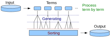
Figure 3: Graphical representation of the processing of an input expression in FORM.

The fundamental objects which are manipulated by FORM commands are expressions which are viewed as sums of individual terms (see also Fig. 3). Next to a sophisticated pattern matcher, it is the strength of FORM that only local operations on single terms are allowed, like replacing parts of a term by some other expressions. Non-local operations like replacing a sum of two terms are not allowed. For example, the command identify (short: id) identifies the left-hand side with the right-hand side and can be used as

  id a = b + c;

On the other hand, the usage

  id a + b = c;

would lead to an error message.

Non-local operations are allowed only implicitly, e.g., in the sorting procedure at the end of the modules, where equivalent terms are combined. At first sight this seems to be a strong limitation for the formulation of general and efficient algorithms. It is usually possible to get around this limitation by designing algorithms in clever and non-standard ways.

Due to the locality of the operations it is possible to handle expressions as “streams” of terms that can be read sequentially from the memory or a file and processed independently. This enables FORM to deal with expressions that are larger than the available main memory.

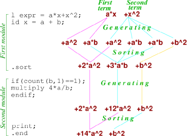
Figure 4: Example for the generation and sorting of data in FORM.

An example illustrating the principle operating mode of a FORM program is shown in Fig. 4. It corresponds to the simple program

  l expr = a*x + x^2;
  id x = a + b;
  .sort
  if (count(b,1)==1);
    multiply 4*a/b;
  endif;
  print;
  .end

4 ParFORM

4.1 The concept of ParFORM

As mentioned above, the locality principle enables FORM on the one hand to deal with expressions that are larger than the available main memory, on the other hand it also allows for parallelization. The concept implemented in ParFORM is straightforward and indicated in Fig. 5: in a first step the master process splits the expression into pieces, so-called chunks. Each chunk is sent to one of the workers where an independent FORM process runs, i.e. the module to be executed is compiled, the terms are generated, sorted and sent back to the master. Once all worker processes have finished their jobs the master performs the final sorting.

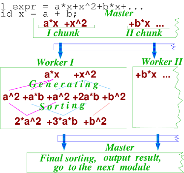
Figure 5: General conception of ParFORM.

The communication between master and workers is based on the message passing interface (MPI) standard [42] which provides a library for the data transfer between processes. Message passing permits to parallelize FORM on computer architectures both with shared memory, i.e. SMP computers and on computer clusters. The way the master communicates with the workers is sketched in Fig. 6.

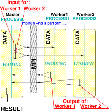
Figure 6: Visualization of the mode of operation of ParFORM based on MPI.

It is worth mentioning that the parallelization does not require any additional efforts from the user. It is possible to run the programs written for the sequential version using ParFORM and adding a specification concerning the number of processors. It is clear that different codes show a different performance and efficiency in the parallel version. In particular, modules in which the outcome depends on the order in which the terms are processed cannot be parallelized and are executed in sequential mode. This concerns mostly the use of the dollar variables which were introduced in version 3. In the case that FORM would switch to sequential mode, while actually this is not needed, the user can add an extra statement to overrule such a decision and tell FORM how to deal with the ‘dubious’ case.

4.2 ParFORM on a NUMA architecture

The SGI Altix computer is realized with a so-called NUMA architecture where NUMA stands for non-uniform memory access. This means that the individual processors have a faster access to some parts of the main memory than to others. A specialized version of ParFORM has been developed which exploits the feature and, at the same time, does not use MPI and the overhead connected to it. The corresponding scheme of operation is illustrated in Fig. 7.

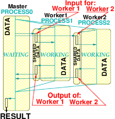
Figure 7: Mode of operation implemented into ParFORM for a NUMA architecture.

Using the specialized version of ParFORM in connection with the 32-core SGI Altix a considerable improvement of the speedup could be obtained, as can be seen in Fig. 8. In fact, for 16 processors the speedup improved from 8 to 10, for 32 processors from 10 to 13 (see also the discusion in the next subsection).

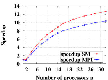
Figure 8: Runtime and speedup for the test program BAICER running on a SGI Altix 3700 server with 32 Itanium-2 processors (1.3 GHz). The lower curve corresponds to the MPI version and the upper one to the shared memory version of ParFORM.

4.3 ParFORM on clusters and multi-core nodes

At present, there are a number of calculations of physical quantities which would not have been possible without the gain in performance and speedup provided by ParFORM (see, e.g., Refs. [34, 14]). Most of the applications are connected to the evaluation of four-loop Feynman integrals which occur in the context of perturbative quantum field theory. In particular, there are algorithms which transform the mathematical complexity of the original problem to the need of simple manipulations of rather large polynomial expressions which have billions or even more terms. Manipulations of this type constitute the basis of the speedup curves which are discussed in the following.

The results for the test program running on a SGI Altix 3700 server with 32 Itanium-2 processors are shown in Fig. 8 where both the runtime and the speedup (as compared to the sequential version) is shown as a function of the number of processors, $p$, involved in the calculation. The almost horizontal line between $p=1$ and $p=2$ is due to the fact that for $p=2$ one of the processors takes over the role of the master and the other one of the worker. Thus a real reduction of the CPU time only starts from $p=3$. It is interesting to note that the speedup is almost linear up to twelve processors. Furthermore, for 16 processors the program is faster by an order of magnitude. As a consequence instead of years one only has to wait a few months in order to obtain the results of a calculation. This provides the possibility to consider qualitatively new kinds of problems, since in practice it is impossible to run a job for years whereas a few months are feasible nowadays. Beyond $p=16$ the curve becomes more flat, however, the speedup is still considerable up to 32 processors.

The latest speedup plot for (the MPI version of) ParFORM is shown in Fig. 9 where BAICER is running on the cluster ttpmoon which has the following configuration:

• Computer cluster (TTP Karlsruhe) running Linux, 8 nodes with 2 Hexa-Core Intel Xeon X5675 (3.07 GHz), 96 GB RAM, and 3.6 TB local hard disk (Raid 0 with 6 stripes), interconnected by QDR InfiniBand.

The top plot shows the used time in minutes as a function of the involved CPUs (including the master) and on the bottom the speedup as compared to the serial version is plotted. It is interesting to note that a speedup of about 10 is reached in case 16 CPUs are used, a value obtained in Fig. 8 for the shared memory version which avoids the use of MPI, cf. Subsection 4.2. For higher number of CPUs the curve flattens but nevertheless reaches a speeup above 20 for 96 CPUs.

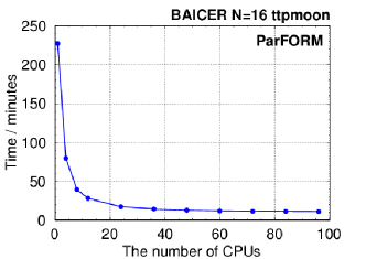
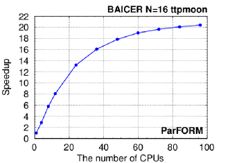
Figure 9: Timing and speedup plot for the ParFORM benchmark job BAICER running of ttpmoon.

4.4 ParFORM on “low-level” clusters

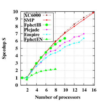
Figure 10: The speedup for the test program on different clusters in comparison to the SMP computer (cf. Fig. 8).

ParFORM has been successfully installed on several clusters. In Fig. 10 the corresponding speedup curves are shown and compared to the curve from Fig. 8 obtained on the SMP computer. The cluster XC6000 is a Hewlett Packard Itanium-2 QsNet interconnected cluster. This is the only tested cluster which demonstrates a better behaviour than the SMP computer, however, it is also significantly more expensive. Fphctl is a cluster consisting of 32-bit Xeon nodes. This cluster has been tested both with an Infiniband (FphctlIB) and a simple Fast Ethernet (FphctlEN) interconnection. Whereas the latter is not of interest in practice the former shows a quite reasonable behaviour following closely the SMP curve for a smaller number of processors. Plejade and Empire are both dual Opteron clusters. However, Plejade is interconnected using InfiniBand whereas Empire uses Gigabit Ethernet. Both clusters show a reasonable behaviour leading to a speedup of about six for ten processors.

We want to mention that the SMP curves shown in Fig. 10 are based on the shared-memory model mentioned above. On the other hand, for the clusters one has to rely on the MPI library which for our applications has a significant overhead.

5 TFORM

In the last decade multi-core processing has become a key technology in the computing industry as system performance improvement through increasing clock rates of single-core processors is hindered by physical limits. From laptops to supercomputers multi-core processing is prevalently used and the modern operating systems allow one to easily use them as SMP computers. Although ParFORM works on such SMP computers, interprocess communications among the master and the workers via MPI can have a significant overhead when gigantic expressions are transfered.

This overhead problem can be overcome on SMP architectures with the help of another model for the communication. In this approach the master explicitly allocates shared memory buffers which can be accessed both by the master and the workers. In these memory segments the master prepares the chunks for the workers, they are doing their job and the master collects the results again from the shared buffers. Thus, copying huge amounts of data is not necessary any more. The use of the shared-memory model on SMP machines led to an increase in the speedup of 20-25% (cf. Fig. 8). This concept is taken even further in TFORM [12], a multithreaded version of FORM.

In TFORM the implementation uses the POSIX threads library, which is available on all modern UNIX systems and therefore portable. The way the master communicates with the workers is sketched in Fig. 11. TFORM starts with one master thread and $N$ worker threads in a so-called thread pool. The workers sleep until the master assigns tasks, and hence do not spend any CPU time. When the master has some task to be distributed over the workers, the master wakes up one of the sleeping workers and assigns the task to it. Terms in expressions, grouped as chunks for reducing the overheads, are distributed in this way. After distributing all terms, the master waits for all the workers to finish the tasks, and then the master merges the results of the workers in a final sorting operation. The data transfer among the threads is done via the shared memory buffers and by using memory locks for synchronization between the master and the workers (see Fig. 11).

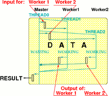
Figure 11: Mode of operation for TFORM.

Due to the model for the communications, some features improving the performance are relatively easy to implement in TFORM, whereas their implementations are difficult in ParFORM. One of them is a load balancing system. If there is a single worker that is assigned terms requiring much CPU time, for the final sorting the master may have to wait for this worker even after the other workers finish their tasks and become idle. To avoid such inefficiency, after distributing all terms to be processed, the master looks for idle workers. If such workers are found, terms are stolen back from the chuncks of workers that are still busy and redistributed over idle workers. Experiments with an even more fine-grained load balancing were unsuccessful, because they resulted in too much overhead.

Another feature in TFORM concerns the parallel sorting. In the final sorting, TFORM used to adopt the simple model in which the master merges the outputs from all the workers simultaneously. Therefore it often happens that the master is busy while the workers are waiting for the master to accept their next chunks of the results. It becomes a bottleneck, especially when the number of the workers is large. To alleviate this bottleneck, an improved model of the final sorting has been implemented in TFORM. In this model, each two workers send their results to a special worker thread, called a sortbot, which merges the results. Then each two sortbots send their results to another sortbot. This continues until the last two sortbots send their results to the master, which merges the final two results and writes the result to disk. This is illustrated in Fig. 12. Because also this method still involves much waiting, a run with $N$ workers will rarely use more than the CPU time provided by $N$ cores, even when the computer has many more cores. The total wall clock execution time improves measurably by this method, although it does go at the cost of extra memory needed for the buffers of the sortbots.

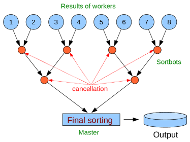
Figure 12: Illustration of the mode of operation of sortbots.

Fig. 13 shows up-to-date timing and speedup plots for ParFORM and TFORM running on ttpmoon. Note that the cluster ttpmoon consists of 12-core nodes which explains the end point of the TFORM curves where a speedup better than 9 is reached. ParFORM reaches for 12 CPUs, which means 1 master and 11 workers, a speedup of 8.

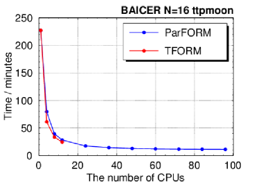
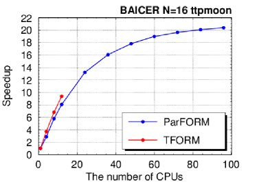
Figure 13: Comparison of timing and speedup for ParFORM and TFORM running on ttpmoon.

6 Further developments within CRC/TR 9

6.1 Reduction to master integrals with FIRE

Nowadays the vast majority of calculations of higher order quantum corrections involve a huge number (sometimes exceeding several millions) of different contributing integrals. The standard way to reduce their number to a manageable amount is based on the so-called “Laporta algorithm” which is described in Ref. [43]. There are many different implementations of this algorithm, some of them are publicly available like AIR [44] or Reduze [45, 46], others are private like crusher [47] which has been developed in the context of project A1 of the CRC/TR 9. Within project A2 the program FIRE [48, 49, 50, 51] has been developed.

FIRE stands for Feynman Integral REduction and implements a special version of the Gauss elimination method to solve the system of linear equations, which is generated by the application of the integration-by-parts relations [52], for the master integrals. It uses several external programs like Snappy [53] for data compression, KyotoCabinet [54] as database to store data on disk, Fermat [36] for algebraic simplifications, and LiteRed [55] to retrieve additional rules among integrals.

The operation of FIRE is divided into two parts: in a first step the input for the reduction step is prepared within Mathematica. This includes the generation of all integration-by-parts relations, the generation of symmetry relations, the identification of the sectors of indices where integrals vanish, i.e. the so-called boundary conditions, and the preparation of a list of integrals which shall be reduced. The second step is significantly more time consuming. In the latest version, FIRE5 [50], this part is written in C++. Here the systematic reduction to master integrals is performed. The output is a table for the list of integrals provided in part one.

Figure 14: Integral family with three massive (double lines), three massless lines and an irreducible numerator (not shown). It it evaluated in forward-scattering kinematics, i.e., there is one external momentum, $p_{1}$, flowing through the upper massless line and another, $p_{2}$, through the lower massive lines.

To demonstrate the use of FIRE let us, for example, consider the integral family of Fig. 14 which has three massive internal lines (with mass $m$). For the external momenta we have $p_{4}=p_{1}$, $p_{3}=p_{2}$ with $p_{1}^{2}=p_{2}^{2}=0$. Integrals of that type contribute to the next-to-leading order corrections to double-Higgs boson production. In fact, the imaginary part, which is a function of $x=m^{2}/s$ (with $s=(p_{1}+p_{2})^{2}$), is related to the total cross section via the optical theorem. The input for the Mathematica part of FIRE contains the following elements (for a detailed description of the commands we refer to Ref. [50]):

(* load FIRE: *)
Get["FIRE5.m"];

(* define integral family: *)
Propagators = {m^2 - (v1-v2)^2,
  m^2 - (p2-v1)^2, m^2 - (p2-v2)^2,
  -v2^2, -v1^2, -(p1+v1)^2, -(p1+v2)^2};
Internal = {v1,v2};
External = {p1,p2};

(* IBP relations: *)
PrepareIBP[];
kinset = {p1^2 -> 0, p2^2 -> 0,
          p1*p2 -> s/2};
set1 = Internal;
set2 = Join[Internal,External];
ncount = 0;
startinglist = {};
For[ii=1,ii<=Length[set1],ii++,
    For[jj=1,jj<=Length[set2],jj++,
        ncount = ncount + 1;
        ff[ncount] =
          IBP[set1[[ii]], set2[[jj]]
            ] /. kinset;
        startinglist =
          Join[startinglist,{ff[ncount]}];
        ];
];

(* boundary conditions: only contributions
   with cuts through at least 2 Higgs
   lines are kept: *)
(RESTRICTIONS = { {0,-1,0,0,0,-1,0},
  {0,0,-1,0,0,0,-1},{0,0,0,0,0,-1,-1},
  {-1,0,0,0,0,0,0},{-1,-1,0,0,0,0,0},
  {-1,0,-1,0,0,0,0},{0,-1,-1,0,0,0,0} });
SYMMETRIES = { {1,3,2,5,4,7,6} };
Prepare[];

(* save data to top2l2h1a.start: *)
SaveStart["top2l2h1a"];

The last command writes all generated information into the so-called “start” file which, together with the list of integrals, serves as input for the reduction step. The steering file, top2l2h1a.config, for the latter has the following form

#threads    4
#variables  d,s,m
#start
#problem    1|7|top2l2h1a.start
#integrals  top2l2h1a.ind
#output     top2l2h1a.tab

where we refer to Ref. [50] for the precise meaning of the individual commands. The integrals which shall be reduced can be found in the file top2l2h1a.ind which might have the form

{{1, {1, 1, 1, 2, 2, 2, 2}},
 {1, {1, 1, 1, 1, 1, 1, 2}},
 {1, {1, 1, 1, 1, 1, 1, -1}}}

Here the individual entries are lists where the integer in the first entry numbers the family and the second entry contains seven integers specifying the indices of the propagators as specified above (see “Propagators”). The reduction is initiated with the help of ./FIRE5 -c top2l2h1a. After the job is completed the reduction table can be found in the file top2l2h1a.tab which can be read using again a Mathematica session of FIRE.

There are several benchmark calculations which have been performed with the help of FIRE. Among them is the reduction of all three-loop integrals needed for the static potential [56, 57, 58] which involves eight indices for massless relativistic propagators and in addition three indices for static propagators of the form $1/k_{0}$. A particular challenge poses the case for general QCD gauge parameter $\xi$ which involves about 20 million integrals, 60 times as much as the $\xi=0$ case. A further reduction problem involves four-loop on-shell integrals needed for the relation between the $\overline{\rm MS}$ and on-shell quark mass relation or the electron anomalous magnetic moment (see, e.g., Ref. [59]).

6.2 Numerical evaluation of master integrals with FIESTA

FIESTA [60, 61, 62] stands for Feynman Integral Evaluation by a Sector decomposiTion Approach and is a convenient tool to numerically evaluate Feynman integrals using the method of sector decomposition. The latter is an algorithmic procedure to extract the $\epsilon$ poles of a given Feynman integral in the so-called alpha-representation and provide an integral representation for the coefficients. After the pioneering work of Binoth and Heinrich [63, 64] several programs have been published where different strategies have been implemented. Among them are sector_decomposition [65], secdec [64, 66, 67], and FIESTA [60, 61, 62].

The basic philosophy of FIESTA is that all kinematic variables are specified at an early stage which is different from other approaches like, e.g., secdec, where generic manipulations are performed up to a certain point and only then numerical values for masses and momenta are specified.

The use of FIESTA splits into the following two steps: In a first step the momentum integrals are transformed into the alpha-representation and the sector decomposition algorithm is applied. The corresponding manipulations are performed in Mathematica and can be done in parallel mode. For many applications this step is quite fast, however, quite often, in particular at higher loop order, huge expressions are generated which require main memory in the range of hundred Gigabyte. In such cases it is convenient to store the results into a database [54] since in general this step has to be performed only once.

The second step is concerned with the numerical integration. In principle this can also be performed within Mathematica, which is advantageous for small problems or during the developing phase of the program. Complicated problems have to be integrated with the help of a C++ integrator which is based on the Cuba library [68, 69]. It uses the expressions stored in the database during step one which provides several advantages. For example, it is possible to perform various runs choosing different values for the number of points used for the integrations. Furthermore, it is possible to copy the output of step one to a platform which is suitable for the numerical integration in massive parallel mode.

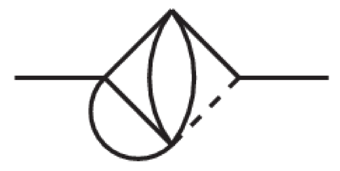
Figure 15: Sample on-shell Feynman diagram where solid and dashed lines denote massive and massless lines, respectively.

Let us as an example consider the Feynman diagram in Fig. 15 which enters the four-loop relation between the $\overline{\rm MS}$-on-shell quark mass. Executing the Mathematica file

Get["FIESTA3.m"];
NumberOfSubkernels=8;
NumberOfLinks=8;
UsingC=True;
UsingQLink=True;
ComplexMode=False;
SDEvaluate[ UF[ {k1,k2,k3,k4},
                {-(k1+q1)^2+m^2,
                 -(k3+q1)^2+m^2,
                 -(k1-k2)^2+m^2,
                 -(k2-k3)^2+m^2,
                 -(k1-k4)^2+m^2,
                 -k4^2+m^2,
                 -k3^2},
                {m->1,q1^2->1}],
                {1,1,1,1,1,1,1},6]

prepares both the integrand and performs the numerical integration using the corresponding C routines in the background. The result which is printed on the screen reads

-276.907674 - 0.625006/ep^4 -
 4.937615/ep^3 + (-24.441689 +
 0.002*pm69)/ep^2 + (-85.919995 +
 0.015937*pm70)/ep + 0.083469*pm71 +
 ep*(-864.271585 + 0.468742*pm72) +
 ep^2*(-1503.357843 + 2.093833*pm73) +
 ep^3*(-6224.681821 + 9.755544*pm74) +
 ep^4*(11328.088699 + 40.591518*pm75) +
 ep^5*(-18622.607506 + 176.767061*pm76) +
 ep^6*(537473.776134 + 713.790523*pm77)

The symbols pm indicate the uncertainty due to the Monte Carlo integration. In case the option OnlyPrepare = True; is added to the Mathematica file the integrand is prepared and stored to disk. Furthermore the command is printed on screen which invokes the numerical integration from the shell without reference to Mathematica.

The result from runs performed at the High Performance Computing Center Stuttgart (HLRS) are shown in Fig. 16 where the speedup for the individual $\epsilon^{n}$ terms ($n=-3,\ldots,6$) is shown. The blue (dotted), green (dashed), red (dash-dotted) and black (solid) curves (from bottom to top) corresponds to the use of 64, 128, 256 and 512 cores where the results have been normalized to the 32-core run. It is interesting to note that an ideal speedup is obtained for 64 cores. Also for 128 cores the curve is close to the maximal value of 4. Using 256 instead of 32 cores still shows a quite flat behaviour with a speedup between 6 and 7. Strong variations in the speedup are observed for the use of 512 cores. The relatively low value for $1/\epsilon^{-3}$ can be explained with the fact that probably the expression, which shall be integrated, is too simple. On the other hand, for the (complicated) expression of the $\epsilon^{6}$ coefficient it might be that the disk access becomes the bottle neck.

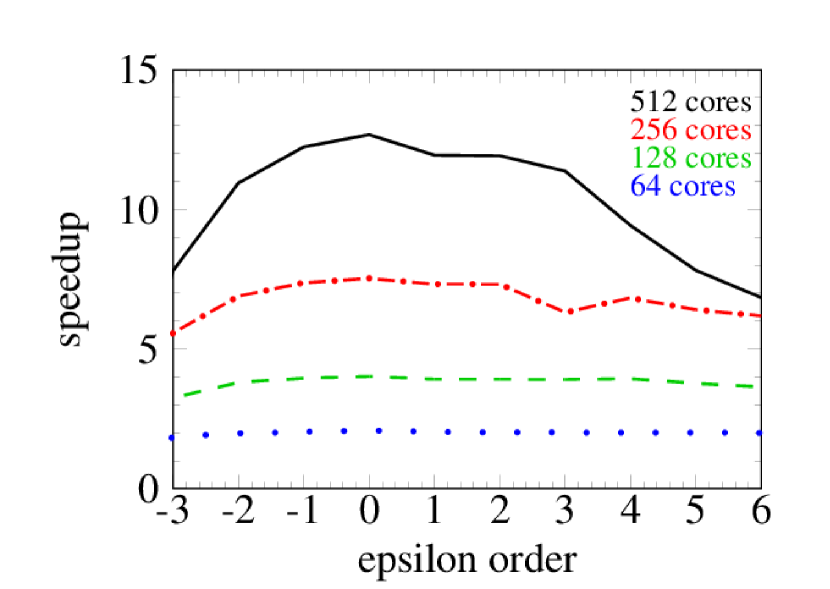
Figure 16: Speedup of the calculation of the various $\epsilon$ orders of Feynman diagram given in Fig. 15 using 64 (dotted), 128 (dashed), 256 (dash-dotted) and 512 (solid) cores normalized to the 32-core run.

The main purpose of FIESTA is the fast and convenient cross check of analytic calculations. Within CRC/TR 9 is has been applied in this way to several problems. An early version of FIESTA has been used to cross check the master integrals which contribute to the three-loop static potential [56, 57, 58]. Furthermore thirteen four-loop on-shell integrals contributing to the $\overline{\rm MS}$-on-shell quark mass relation and to the muon anomalous magnetic moment, which have been computed analytically in Ref. [59], have been cross-checked numerically with FIESTA. Recently also analytic results for master integrals of double-box topologies in the physical region have been cross-checked with the help of FIESTA [70].

There are also several projects where FIESTA has been used to evaluate the most complicated or even the major part of the master integrals numerically. For example, in the first calculation of the three-loop corrections of the quark and gluon form factor [22] (see also Ref. [71]) one coefficient in the $\epsilon$ expansion of the three most complicated integrals could not be evaluated analytically. Thus, the numerical results of FIESTA have been used which, for all practical purposes, leads to final results with sufficient precision. The analytic calculation of the missing master integrals has been performed in Ref. [72] and perfect agreement with the numerical result has been found.

For the calculation of the three-loop matching coefficient between QCD and non-relativistic QCD (NRQCD) of the vector current [73] even the majority of the about 100 master integrals have been computed numerically with the help of FIESTA. In such cases it is important to perform strong cross checks. Among them are the change of the parametrization of the individual integrals. Thus, in intermediate steps different expressions are generated which are then integrated numerically. Furthermore, it is possible to choose a different integrals basis and evaluate the new integrals again with the help of FIESTA. The agreement of the final expression within the numerical uncertainty among the two set of master integrals serves as a strong checked for the applicability of FIESTA.

7 Summary

The computer algebra program FORM is designed to handle huge expressions in a quite effective way. Still, for some physical applications even FORM would take several years which make a practical calculation impossible.

In the recent years parallel versions of FORM, ParFORM and TFORM, have been developed and in the meantime they have become a reliable tools to perform computer algebra in parallel. ParFORM has demonstrated a good speedup behaviour both on SMP computers and on different cluster architectures. Furthermore, for the current version of ParFORM the FORM programs written for the sequential version need not to be modified.

TFORM is a parallel version of FORM based on POSIX threads and thus is bound to run on a single node. However, there is less overhead connected to the parallelization and thus TFORM shows a slightly better performance than ParFORM.

The main advantage of using a parallel version of FORM is the reduction of the wall clock time. In fact, there are a number of calculations where it has been exploited that a speedup of about 10 can be reached with 16 cores and thus the result was available after about a month instead of a year. A further advantage of using TFORM or ParFORM is the fact that the size of the intermediate results, which have to be handled by the individual CPU, is smaller since the workload is distributed among several workers. This advantage becomes particularly evident when using ParFORM on a cluster. In that case the intermediate expressions are stored into files which are located on different nodes.

To obtain an even better speedup behaviour it would be necessary to improve the slope of the speedup curves and to push the flattening to higher number of processors. One starting point which could help to improve the situation is the sorting procedure. Another idea might be the combination of ParFORM and TFORM which could be an ideal tool for a cluster with multi-core nodes.

In this article we also describe the programs FIRE and FIESTA. FIRE can be used for the reduction of integrals belonging to a given integral family to master integrals. FIESTA, on the other hand is a user-friendly tool to numerically compute the coefficients of the $\epsilon$ expansion of multi-loop integrals.

References

- [1] A. C. Hearn, PRINT-71-1192; reduce-algebra.com
- [2] M. J. G. Veltman, Schoonschip, CERN Report 1967.
- [3] H. Strubbe, Comput. Phys. Commun. 8 (1974) 1; Comput. Phys. Commun. 18 (1979) 1.
- [4] M. J. G. Veltman and D. N. Williams, hep-ph/9306228.
- [5] M.I.Levine, ASHMEDAI, Comput. Phys. I (1967) 454; R. C. Perisho, ASHEMEDAI users guide, U.S. AEC Report No. COO-3066-44, 1975.
- [6] www.symbolics-dks.com/Macsyma-1.htm; for the open-source version see maxima.sourceforge.net
- [7] www.wolfram.com/mathematica
- [8] www.maplesoft.com
- [9] J. A. M. Vermaseren, math-ph/0010025.
- [10] J. Kuipers, T. Ueda, J. A. M. Vermaseren and J. Vollinga, Comput. Phys. Commun. 184 (2013) 1453 [arXiv:1203.6543 [cs.SC]].
- [11] M. Tentyukov, D. Fliegner, M. Frank, A. Onischenko, A. Retey, H. M. Staudenmaier and J. A. M. Vermaseren, cs/0407066 [cs-sc].
- [12] M. Tentyukov and J. A. M. Vermaseren, Comput. Phys. Commun. 181 (2010) 1419 [hep-ph/0702279 [HEP-PH]].
- [13] P. A. Baikov, K. G. Chetyrkin and J. H. Kühn, Phys. Rev. D 67 (2003) 074026 [hep-ph/0212299].
- [14] P. A. Baikov, K. G. Chetyrkin and J. H. Kühn, Phys. Lett. B 559 (2003) 245 [hep-ph/0212303].
- [15] P. A. Baikov, K. G. Chetyrkin and J. H. Kühn, Nucl. Phys. Proc. Suppl. 116 (2003) 78.
- [16] P. A. Baikov, K. G. Chetyrkin and J. H. Kühn, Eur. Phys. J. C 33 (2004) S650 [hep-ph/0311137].
- [17] P. A. Baikov, K. G. Chetyrkin and J. H. Kühn, Phys. Rev. Lett. 95 (2005) 012003 [hep-ph/0412350].
- [18] K. G. Chetyrkin and A. Khodjamirian, Eur. Phys. J. C 46 (2006) 721 [hep-ph/0512295].
- [19] P. A. Baikov, K. G. Chetyrkin and J. H. Kühn, Phys. Rev. Lett. 96 (2006) 012003 [hep-ph/0511063].
- [20] P. A. Baikov and K. G. Chetyrkin, Phys. Rev. Lett. 97 (2006) 061803 [hep-ph/0604194].
- [21] P. A. Baikov, K. G. Chetyrkin and J. H. Kühn, Phys. Rev. Lett. 101 (2008) 012002 [arXiv:0801.1821 [hep-ph]].
- [22] P. A. Baikov, K. G. Chetyrkin, A. V. Smirnov, V. A. Smirnov and M. Steinhauser, Phys. Rev. Lett. 102 (2009) 212002 [arXiv:0902.3519 [hep-ph]].
- [23] P. A. Baikov, K. G. Chetyrkin and J. H. Kühn, Phys. Rev. Lett. 104 (2010) 132004 [arXiv:1001.3606 [hep-ph]].
- [24] P. A. Baikov, K. G. Chetyrkin, J. H. Kühn and J. Rittinger, Phys. Rev. Lett. 108 (2012) 222003 [arXiv:1201.5804 [hep-ph]].
- [25] P. A. Baikov, K. G. Chetyrkin, J. H. Kühn and J. Rittinger, JHEP 1207 (2012) 017 [arXiv:1206.1284 [hep-ph]].
- [26] P. A. Baikov, K. G. Chetyrkin, J. H. Kühn and J. Rittinger, Phys. Lett. B 714 (2012) 62 [arXiv:1206.1288 [hep-ph]].
- [27] P. A. Baikov, K. G. Chetyrkin and J. H. Kühn, arXiv:1402.6611 [hep-ph].
- [28] J. Blumlein, D. J. Broadhurst and J. A. M. Vermaseren, Comput. Phys. Commun. 181 (2010) 582 [arXiv:0907.2557 [math-ph]].
- [29] A. Vogt, S. Moch and J. A. M. Vermaseren, PoS LL 2014 (2014) 040 [arXiv:1405.3407 [hep-ph]].
- [30] S. Moch, J. A. M. Vermaseren and A. Vogt, Nucl. Phys. B 889 (2014) 351 [arXiv:1409.5131 [hep-ph]].
- [31] D. Fliegner, A. Retey and J. A. M. Vermaseren, hep-ph/9906426.
- [32] D. Fliegner, A. Retey and J. A. M. Vermaseren, hep-ph/0007221.
- [33] S. A. Larin, F. V. Tkachov and J. A. M. Vermaseren, NIKHEF-H-91-18.
- [34] A. Retey and J. A. M. Vermaseren, Nucl. Phys. B 604 (2001) 281 [hep-ph/0007294].
- [35] M. Tentyukov and J. A. M. Vermaseren, Comput. Phys. Commun. 176 (2007) 385 [cs/0604052 [cs-sc]].
- [36] https://home.bway.net/lewis/
- [37] J. A. M. Vermaseren and M. Tentyukov, Nucl. Phys. Proc. Suppl. 160 (2006) 38.
- [38] M. Tentyukov and J. A. M. Vermaseren, PoS ACAT 08 (2008) 119.
- [39] M. Tentyukov, J. A. M. Vermaseren and J. Vollinga, PoS ACAT 2010 (2010) 072 [arXiv:1006.2099 [hep-ph]].
- [40] M. Tentyukov, H. M. Staudenmaier and J. A. M. Vermaseren, Nucl. Instrum. Meth. A 559 (2006) 224.
- [41] J. Kuipers, T. Ueda and J. A. M. Vermaseren, Comput. Phys. Commun. (2014) [arXiv:1310.7007 [cs.SC]].
- [42] www.mpi-forum.org
- [43] S. Laporta, Int. J. Mod. Phys. A 15 (2000) 5087 [hep-ph/0102033].
- [44] C. Anastasiou and A. Lazopoulos, JHEP 0407 (2004) 046 [hep-ph/0404258].
- [45] C. Studerus, Comput. Phys. Commun. 181 (2010) 1293 [arXiv:0912.2546 [physics.comp-ph]].
- [46] A. von Manteuffel and C. Studerus, arXiv:1201.4330 [hep-ph].
- [47] P. Marquard and D. Seidel, unpublished.
- [48] A. V. Smirnov, JHEP 0810 (2008) 107 [arXiv:0807.3243 [hep-ph]].
- [49] A. V. Smirnov and V. A. Smirnov, Comput. Phys. Commun. 184 (2013) 2820 [arXiv:1302.5885 [hep-ph]].
- [50] A. V. Smirnov, arXiv:1408.2372 [hep-ph].
- [51] http://science.sander.su/FIRE.htm
- [52] K. G. Chetyrkin and F. V. Tkachov, Nucl. Phys. B 192 (1981) 159.
- [53] https://code.google.com/p/snappy/
- [54] http://fallabs.com/kyotocabinet/
- [55] http://www.inp.nsk.su/~lee/programs/LiteRed/
- [56] A. V. Smirnov, V. A. Smirnov and M. Steinhauser, Phys. Lett. B 668 (2008) 293 [arXiv:0809.1927 [hep-ph]].
- [57] A. V. Smirnov, V. A. Smirnov and M. Steinhauser, Phys. Rev. Lett. 104 (2010) 112002 [arXiv:0911.4742 [hep-ph]].
- [58] C. Anzai, Y. Kiyo and Y. Sumino, Phys. Rev. Lett. 104 (2010) 112003 [arXiv:0911.4335 [hep-ph]].
- [59] R. Lee, P. Marquard, A. V. Smirnov, V. A. Smirnov and M. Steinhauser, JHEP 1303 (2013) 162 [arXiv:1301.6481 [hep-ph]].
- [60] A. V. Smirnov and M. N. Tentyukov, Comput. Phys. Commun. 180 (2009) 735 [arXiv:0807.4129 [hep-ph]].
- [61] A. V. Smirnov, V. A. Smirnov and M. Tentyukov, Comput. Phys. Commun. 182 (2011) 790 [arXiv:0912.0158 [hep-ph]].
- [62] A. V. Smirnov, Comput. Phys. Commun. 185 (2014) 2090 [arXiv:1312.3186 [hep-ph]].
- [63] T. Binoth and G. Heinrich, Nucl. Phys. B 680 (2004) 375 [hep-ph/0305234].
- [64] T. Binoth and G. Heinrich, Nucl. Phys. B 693 (2004) 134 [hep-ph/0402265].
- [65] C. Bogner and S. Weinzierl, Comput. Phys. Commun. 178 (2008) 596 [arXiv:0709.4092 [hep-ph]].
- [66] S. Borowka, J. Carter and G. Heinrich, Comput. Phys. Commun. 184 (2013) 396 [arXiv:1204.4152 [hep-ph]].
- [67] S. Borowka and G. Heinrich, Comput. Phys. Commun. 184 (2013) 2552 [arXiv:1303.1157 [hep-ph]].
- [68] T. Hahn, Comput. Phys. Commun. 168 (2005) 78 [hep-ph/0404043].
- [69] http://www.feynarts.de/cuba/
- [70] F. Caola, J. M. Henn, K. Melnikov and V. A. Smirnov, arXiv:1404.5590 [hep-ph].
- [71] T. Gehrmann, E. W. N. Glover, T. Huber, N. Ikizlerli and C. Studerus, JHEP 1006 (2010) 094 [arXiv:1004.3653 [hep-ph]].
- [72] R. N. Lee and V. A. Smirnov, JHEP 1102 (2011) 102 [arXiv:1010.1334 [hep-ph]].
- [73] P. Marquard, J. H. Piclum, D. Seidel and M. Steinhauser, Phys. Rev. D 89 (2014) 034027 [arXiv:1401.3004 [hep-ph]].