A Gaussian Model for Simulated Geomagnetic Field Reversals

Abstract

Field reversals are the most spectacular changes in the geomagnetic field but remain little understood. Paleomagnetic data primarily constrain the reversal rate and provide few additional clues. Reversals and excursions are characterized by a low in dipole moment that can last for some $10\,$kyr. Some paleomagnetic records also suggest that the field decreases much slower before an reversals than it recovers afterwards and that the recovery phase may show an overshoot in field intensity. Here we study the dipole moment variations in several extremely long dynamo simulation to statistically explored the reversal and excursion properties. The numerical reversals are characterized by a switch from a high axial dipole moment state to a low axial dipole moment state. When analysing the respective transitions we find that decay and growth have very similar time scales and that there is no overshoot. Other properties are generally similar to paleomagnetic findings. The dipole moment has to decrease to about $30$% of its mean to allow for reversals. Grand excursions during which the field intensity drops by a comparable margin are very similar to reversals and likely have the same internal origin. The simulations suggest that both are simply triggered by particularly large axial dipole fluctuations while other field components remain largely unaffected. A model at a particularly large Ekman number shows a second but little Earth-like type of reversals where the total field decays and recovers after some time.

1 Introduction

The geomagnetic field varies over a broad range of time scales raging from one to many million years (Constable and Johnson, 2005). Adequately covering these vastly different time scales is a challenge for geomagnetic data acquisition and numerical dynamo modelling alike. Here we mostly focus on variations in the dipole component and in particular on reversals and excursions. Analysis of Earth’s secular variation in historical and archeomagnetic field models suggests that the typical dipole time scale is about a millennium while higher field harmonics change over centuries or decades (Christensen and Tilgner, 2004; Lhuillier et al., 2011). Paleomagnetic records constrain the longer time scales but suffer from a lack of temporal resolution, ambiguities in dating, and difficulties in determining the paleofield intensity (Hulot et al., 2010). Slow dipole variations are mostly associated to reversals and excursions, a second class of events where the geomagnetic pole ventures further away from the geographic pole but ultimately returns. The associated changes in the dipole tilt last from one to several millennia (Clement, 2004; Valet et al., 2012). Both types of events are characterized by a strong decrease in field intensity likely caused by a drop in axial dipole strength which can last several $10\,$kyr (Valet et al., 2005; Singer et al., 2005; Channell et al., 2009; Amit et al., 2010; Valet et al., 2012). The last reversal, the transition from the Matuyama to the Brunhes polarity chron, happened about $780\,$kyr ago but reversals are stochastic events and their rate has varied greatly over the paleomagnetic history. A particularly long period without any reversal is the Cretaceous normal superchron that lasted about $35\,$Myr but up to $10$ reversals per Myr have also been recorded. Variations in the reversals rate are typically associated to changes in Earth’s lower mantle which have a similar time scale of some $10\,$Myr (Biggin et al., 2012).

Excursions seem to be considerably more frequent than reversals. Up to $17$ excursions have been reported for the Bruhnes (Lund et al., 2001, 2006; Roberts, 2008) and up to $9$ for the Matuyama chron (Channell et al., 2009). Since reversals are bound by longer lasting chrons with opposite polarity they are relatively easy to detect in a paleomagnetic sequence. The exact timing of the reversal may still be difficult but the presence of the chrons is evidence enough. Excursions, however, are only recorded when the temporal resolution of the paleomagnetic medium exceeds their relatively short duration (Roberts and Winklhofer, 2004). The number of documented excursion will likely increase when better quality high-resolution records become available (Roberts, 2008). Additional uncertainties arise from the fact that some excursions may not be global events.

Paleomagnetic records provide local rather than global information. While the local field remains a good proxy for the dipole behaviour during stable polarity epoches this is not necessarily true during reversals and excursions when the relative dipole contribution is low. The likelihood of recording transitional or inverse directions at a given site therefore depends on the multipole field contributions and also increases with duration and depth of the drop in dipole intensity (Wicht, 2005; Wicht et al., 2009). A preponderance of sites with inverse directions during recent excursions could mean that the dipole had started to grow with inverse polarity during these events (Valet et al., 2008). Excursions may thus be abbreviated reversals. Gubbins (1993) suggests that an inverse direction can only be established when the inverse field has a chance to diffuse deep into the inner core. Excursions are then simply events where the period of inverse field production is shorter than the inner core dipole diffusion time of about $7\,$kyr. Dynamo models by (Wicht, 2002), on the other hand, indicate that the highly dynamic dynamo process cares little for the dissipation in Earth’s relatively small inner core but newer simulations addressing this question show contradictory results (Dharmaraj and Stanley, 2012; Lhuillier et al., 2013).

Reversals during the last $2\,$Myr are characterized by a drop in dipole moment from a mean value of around $\overline{M}=7\mbox{$\times 10^{22}$}$A m² to a low around $M_{L}=2\mbox{$\times 10^{22}$}$A m² (Valet et al., 2005; Channell et al., 2009). When analysing high quality sedimentary data for the five most recent reversals, Valet et al. (2005) find that the magnetic field strength decays much slower before actual polarity transition than it grows afterwards. The decay phase lasts about $50\,$kyr and is thus comparable to the core dipole decay time of $t_{d}\approx 56\,$kyr based on newly revised estimates for the electrical conductivity of Earth’s core alloy Pozzo et al. (2012). While the decrease in magnetic field strength could thus be a simple diffusive process this is not the case for the faster recovery which takes less than $10\,$kyr. Some records also suggest that the field intensity overshoots its mean value at the end of the recovery phase (Pétrélis et al., 2009). Neither a significantly faster recovery nor the overshoot have ever been reported for excursions but the drop in field intensity during these events seems comparable to those recorded for reversals (Roberts, 2008; Channell et al., 2009). Ziegler and Constable (2011), however, report that magnetic field decayed on average $20$% faster than it growed during the last $2\,$Myr when considering time scales longer than about $25\,$kyr. The strong site dependence and complex transition behavior during reversals and excursions indicates that the more time dependent higher harmonic contributions dominate at least for some time Singer et al. (2005); Valet et al. (2005, 2012). The drop in field intensity is thus mainly caused by a decrease of the dipole component.

The cause for reversals and excursions remains little understood. Insight comes from paleomagnetic measurements, theoretical considerations, laboratory experiments, and numerical dynamo simulations. Simple dynamical models that manage to reproduce their fundamental stochastic nature include Rikitake coupled disc dynamos (Rikitake, 1958), mean field dynamos (Ryan and Sarson, 2007; Stefani et al., 2007), low order dynamical models (Melbourne et al., 2001; Schmitt et al., 2001; Pétrélis et al., 2009), or a coupled spin system (Mori et al., 2013).

The VKS dynamo is the only experiment that features Earth-like reversals and excursions, including a faster recovery and an overshoot after reversals but not after excursions (Ravelet et al., 2008). The low order model by Pétrélis et al. (2009) manages to explain these differences despite reducing the dynamics to the interaction between only two magnetic field components. The primary component is the axial dipole while the secondary component can be any other field contribution. Configurations with dominant primary field of either polarity form two stable points in phase space that are supplemented by two unstable points with weaker primary and stronger secondary field. Random fluctuations can drive the system away from a stable point towards the closest unstable point, causing a decrease in the axial dipole. When the fluctuations team up constructively enough to cross the unstable point, the system is attracted towards the opposite stable point and a reversal happens. The stochastic variation around the stable point can be understood as a random walk and are thus comparatively slow (Schmitt et al., 2001). The attraction by the opposite attractor beyond the unstable points guarantees a faster recovery and an overshoot towards the second unstable point. Fluctuations short of the unstable points can lead to excursions where the system returns to the original fix point. Both the axial dipole decay and growth phase of an excursion would be slow and there is not overshoot. This dynamics is typical for a system just below a saddle node bifurcation. Beyond the bifurcation, however, stable and unstable points coincide and the system undergoes limit cycles equivalent to continuous reversing (Pétrélis et al., 2009).

Caution is required when transferring the results from such simplified approaches to the geodynamo. Full 3d dynamo simulations feature a more realistic dynamic but suffer from limitations in computing power and problems in interpreting the complex dynamics. The Ekman number, a measure for the relative importance of viscous forces, has to be chosen many orders of magnitude too high to damp the smaller scales that cannot be resolved with the available computing power. This is particularly true for reversal simulations that have to be integrated sufficiently long enough to capture these rare events. Takahashi et al. (2005) present a reversing model at an Ekman number of $\mbox{E}=2\times 10^{-5}$. More typical, however, are larger values up to $2\times 10^{-2}$ (Wicht, 2005; Aubert et al., 2008). Earth’s Ekman number is around $10^{-15}$ (when base on molecular diffusivities) while most advanced dynamo simulations reach $10^{-6}$ but are too short or too weakly driven to show reversals (Wicht et al., 2011).

Numerical parameter studies suggest that sufficiently strong inertial forces are essential for triggering reversals (Christensen and Aubert, 2006; Driscoll and Olson, 2009; Wicht et al., 2009; Olson and Amit, 2014). Christensen and Aubert (2006) demonstrate that this can be quantified in term of the local Rossby number

$$\mbox{Ro}_{\ell}=\mbox{U}/(\Omega d)\;\;.$$ (1)

This modified Rossby number, based on the rms flow amplitude U and a characteristic flow length scale $d$, is a measure for the ratio of inertial to Coriolis forces in the Navier-Stokes equation. The dipole field clearly dominates and is very stable as long as reversal forces are weak. Beyond about $\mbox{Ro}_{\ell}\approx 0.1$, however, the dipole seems to loose its special role, becomes comparable to the other multipole contribution, and reverses more or less continuously. Earth-like reversals where the axial dipole still dominates in a mean sense and reversals and excursions are rare can be found in a narrow $\mbox{Ro}_{\ell}$ interval just before the transition (Wicht et al., 2009). These events thus happen close to a critical point in the parameter space where the system changes its dynamics, a concept discussed by several of the low order dynamical models (Stefani et al., 2007; Pétrélis et al., 2009). Fluctuations in the highly variable flow and magnetic field cause transitions from the stable into the multipolar regime where the dipole reverses more easily (Kutzner and Christensen, 2002). When the system returns, it is just a matter of chance whether the original or the inverse polarity is amplified. Reversals and excursion should thus be equally likely (Wicht et al., 2009). In terms of the simple low order approach by Pétrélis et al. (2009) these events would be described by the limit cycle process flanked but additional dynamical processes that allow to cross the bifurcation. Faster recovery and overshoot may still be possible but am inherent feature of such a model.

No full dynamo simulation has directly addressed the question of a possible asymmetry in dipole decay and growth during reversals or excursions. Lhuillier et al. (2013) analyse five reversing dynamos at an Ekman number of $\mbox{E}=6.5\times 10^{-3}$ with altogether nearly $2000$ reversals. Judging from their figures, neither model shows any faster recovery but one features at least the overshoot. Unfortunately, this model is little Earth-like since it uses an electrically insulating inner core and shows much fewer excursions than reversals. Gissinger et al. (2010) explore a simplified dynamo model where Coriolis force and buoyancy force are replaced by a suitable driving term that produces a reversing dipole dominated field. A faster decay can only be observed when the magnetic Prandtl number Pm, the ratio of viscous to magnetic diffusivity, is below unity. Since the magnetic Prandtl number where dynamo action is still possible decreases with the Ekman number in full dynamo models a Pm below unity can only be reached at $E\leq 10^{-4}$ (Christensen and Aubert, 2006). The model by Takahashi et al. (2005) is the only one in this range and neither the faster recovery not the overshoot are reported. However, their numerical runs cover only few transitions and these issues are not directly addressed.

Most simulations show that the reversal behavior can be very complex and highly variable in time (Glatzmaier et al., 1999; Coe et al., 2000; Kutzner and Christensen, 2002; Wicht, 2005; Wicht et al., 2009; Driscoll and Olson, 2009; Lhuillier et al., 2013). Addressing the properties of reversals and excursions therefore requires a statistical approach based on particularly long simulations with as many simulations as possible. The reversal behavior depends on the convective driving and the thermal boundary conditions used in the numerical model, for example on the outer-boundary heat flux pattern imposed by the lower mantle (Glatzmaier et al., 1999; Kutzner and Christensen, 2004; Olson et al., 2010, 2013). System parameters like Ekman number and Rayleigh number also play an important role (Driscoll and Olson, 2009; Olson and Amit, 2014).

The main purpose of this paper is to analyse the statistical properties of reversals and excursions in several dynamo models and explore whether they reproduce paleomagnetic observations. The models cover Ekman numbers from $\mbox{E}=2\mbox{$\times 10^{-2}$}$ to $\mbox{E}=3\mbox{$\times 10^{-4}$}$ and also differ in Rayleigh number and convective driving mode. We start with explaining the numerical approach in section 2 and introduce the different dynamo models in section 3. Section 4 is devoted to more generally analysing statistical dipole fluctuations at different Rayleigh numbers which lead us to defining a Gaussian model for reversals. Based on this model we proceed with quantifying the properties of reversals and excursions in section 5 and section 6. A discussion in section 8 closes the paper.

2 Numerical Methods

Since the details of the empoyed numerical dynamo model MagIC3 have been explained elsewhere (Wicht, 2002; Christensen and Wicht, 2007) we concentrate on outlining only the essential ingredients here. A coupled system of equations describing convective motions and dynamo action is solved in a rotating spherical shell that represents Earth’s outer core. These equations are the Navier-Stokes equation in the Boussineq approximation (2), the induction equation (3), and a transport equation for codensity $C$ (4). They are supplemented by the simplified continuity equation (6) and the condition (5) that the magnetic field is divergence free:

$$\begin{split}\mbox{E}\,\mbox{Pm}^{-1}\;\left(\,\dot{\mbox{$\mathbf{U}$}}+\mbox{$\mathbf{U}$}\cdot\nabla\mbox{$\mathbf{U}$}\right)-\mbox{E}\;\nabla^{2}\mbox{$\mathbf{U}$}+2\hat{\bf z}\times\mbox{$\mathbf{U}$}+\nabla P=\\ \mbox{Ra}\,\mbox{Pm}\;r/r_{o}C\hat{r}+(\nabla\times\mbox{$\mathbf{B}$})\times\mbox{$\mathbf{B}$}\end{split}$$ (2)

$$\dot{\mbox{$\mathbf{B}$}}=\nabla\times(\mbox{$\mathbf{U}$}\times\mbox{$\mathbf{B}$})+\;\nabla^{2}\mbox{$\mathbf{B}$}$$ (3)

$$\dot{C}+\mbox{$\mathbf{U}$}\cdot\nabla C=\;\mbox{Pm}\,\mbox{Pr}^{-1}\nabla^{2}C+\epsilon$$ (4)

$$\nabla\cdot{\mbox{$\mathbf{B}$}}=0$$ (5)

$$\nabla\cdot{\mbox{$\mathbf{U}$}}=0$$ (6)

$\mathbf{B}$, $\mathbf{U}$, and $P$ are magnetic induction, velocity, and pressure perturbation, respectively. Vectors $\hat{\bf r}$ and $\hat{\bf z}$ denote the unit vectors in radial direction and along the rotation axis and dots over a variable indicate a partial time derivative. The codensity $C$ can stand for the super-adiabatic temperature or the relative contribution of light elements in the outer core. The spherical shell is bounded by an insulating mantle at $r=r_{o}$ and an electrically conducting inner core at $r=r_{i}$ which rotates subject to viscous and Lorentz torques (Wicht, 2002).

The following scales have been used to make above equations dimensionless: The shell thickness $d=r_{o}-r_{i}$ serves as the length scale and the magnetic field is scaled by $(\sigma/\rho\Omega)^{1/2}$, with $\rho$ the outer core density, $\sigma$ the electric conductivity, and $\Omega$ the basic rotation rate. Time is measured in units of the magnetic diffusion time $t_{\lambda}=d^{2}/\lambda$, where $\lambda=(\mu\sigma)^{-1}$, and $\mu$ is the magnetic permeability. The dipole decay time is a fraction of the magnetic diffusion time: $t_{d}=t_{\lambda}r_{o}^{2}/(d^{2}\pi^{2})$. The codensity gradient across the outer core, $\Delta C/d$, serves as a codensity unit in models where $C$ is kept fixed at the boundaries. This is equivalent to imposing a constant temperature gradient $\Delta T=\Delta C/\alpha$ with thermal expansivity $\alpha$. Two setups explore the effects of purely compositional driving from a growing inner core which we model by setting the codensity flux through the outer boundary to zero. The sink term $\epsilon$ in eqn. (4) is then used to balance the codensity flux from the inner core and also serves as a codensity scale. Rigid flow boundary conditions are used in all models.

The numerical model then comprises five dimensionless numbers: The Ekman number $E=\nu/\Omega d^{2}$, the (modified) Rayleigh number $Ra=g_{o}\delta Cd/\nu\Omega$, the Prandtl number $\mbox{Pr}=\nu/\kappa$, the magnetic Prandtl number $\mbox{Pm}=\nu/\lambda$, and the aspect ratio $a=r_{i}/r_{o}$.

Name	Revs.	E	Pm	BC	Ra	Ra/Rac	Rm	$\Lambda_{\mbox{{\scriptsize CMB}}}$	$\mbox{Ro}_{\ell}$	$\mbox{D}_{geo}$	${\tau}_{T}$	${{\tau}_{A}}$	$N_{R\theta}$	$N_{E\theta}$	$N_{e\theta}$
E3R5	-	$10^{-3}$	$10$	temp.	$250$	$4.5$	$202$	$2.6$	$0.04$	$0.60$	$0.00$	$137$	0	0	0
E3R7	-				$400$	$7.2$	$350$	$2.0$	$0.09$	$0.44$	$0.00$	$58$	0	0	0
E3R8	E				$450$	$8.1$	$393$	$1.8$	$0.11$	$0.38$	$0.01$	$87$	4	1	10
E3R9	E				$500$	$8.9$	$436$	$1.5$	$0.12$	$0.31$	$0.04$	$4\,208$	542	613	1963
E3R13	M				$750$	$13.4$	$592$	$1.7$	$0.17$	$0.18$	$0.34$	$55$	–	–	–
E3R9C	-	$10^{-3}$	$10$	chem.	$500$	$9.4$	$229$	$2.1$	$0.05$	$0.57$	$0.00$	$98$	0	0	0
E3R19C	-				$1000$	$18.8$	$374$	$1.2$	$0.09$	$0.42$	$0.00$	$77$	0	1	3
E3R23C	E				$1250$	$23.5$	$442$	$0.65$	$0.11$	$0.30$	$0.05$	$431$	105	104	234
E3R28C	M				$1500$	$28.2$	$491$	$0.56$	$0.12$	$0.23$	$0.18$	$323$	–	–	–
E3R38C	M				$2000$	$37.6$	$564$	$0.71$	$0.14$	$0.19$	$0.42$	$45$	–	–	–
E4R53C	-	$3\mbox{$\times 10^{-4}$}$	$3$	chem.	$3000$	$80$	$264$	$0.34$	$0.09$	$0.66$	$0.00$	$11$	0	0	0
E4R78C	-				$4500$	$120$	$340$	$0.25$	$0.11$	$0.59$	$0.02$	$45$	0	2	1
E4R106C	E				$6000$	$160$	$408$	$0.14$	$0.13$	$0.40$	$0.14$	$87$	20	30	45
E4R159C	M				$9000$	$240$	$497$	$0.15$	$0.16$	$0.27$	$0.10$	$20$	–	–	–
E2R1.8	-	$2\mbox{$\times 10^{-2}$}$	$10$	temp.	$220$	$1.8$	$65$	$0.37$	$0.16$	$0.50$	$0.00$	$1\,342$	0	0	0
E2R2.2	E				$260$	$2.2$	$81$	$0.20$	$0.20$	$0.38$	$0.05$	$1\,220$	160	32	64
E2R2.5	E				$300$	$2.5$	$94$	$0.33$	$0.23$	$0.40$	$0.06$	$9\,583$	2956	948	2279
E2R4.2	M				$500$	$4.2$	$148$	$0.42$	$0.37$	$0.28$	$0.21$	$346$	–	–	–
Earth	E	$10^{-15}$	$10^{-6}$	flux	–	–	$2000$	$O(1)$	$0.09$	$0.79$	$<0.6$	$>12\,000$	–	–

Table 1: List of parameters and time averaged properties for the explored dynamo models and Earth. Column 4 details the driving mechanism: an imposed constant temperature jump across the shell (temp.), or chemical convection (chem.). The Prandtl number is unity in all cases. Magnetic Reynolds number Rm, CMB Elsasser number $\Lambda_{\mbox{{\scriptsize CMB}}}$, local Rossby number $\mbox{Ro}_{\ell}$, and relative CMB dipole strength D_ℓ≤11 are time averaged values. Earth values refer to molecular diffusivities, the GUFM field model, and the local Rossby number estimate by Christensen and Aubert (2006). The relative transitional dipole time ${\tau}_{T}$ in column 12 is the fraction of time the magnetic north pole spends further away from the closest geographic pole than $45^{\circ}$. Column 13 gives the total simulation time in units of dipole diffusion time and the last three columns list the number of reversal, grand excursions, and excursions based on the tilt criterion. See main text for more explanations.

3 Model overview

To study the statistical behaviour of dipole variations and reversals we compiled extremely long simulations of dynamo models at three different Ekman numbers ($2\mbox{$\times 10^{-2}$},10^{-3},3\mbox{$\times 10^{-4}$}$) and different Rayleigh numbers. All models assume a Prandtl number $\Pr=1$ and an Earth-like aspect ratio $a=0.35$. The magnetic Prandtl number is $\mbox{Pm}=3$ for the lowest Ekman number models and $10$ otherwise. Some of these models have previously been discussed in the literature (Kutzner and Christensen, 2002; Wicht, 2005; Wicht and Christensen, 2010). The naming of the models follows the convention $ExR?$ where $x$ is the unsigned exponent in the Ekman number and the question mark stands for the supercriticality $\mbox{Ra}/\mbox{Ra}_{c}$, $\mbox{Ra}_{c}$ being the critical Rayleigh number for onset of convection. A $C$ at the end of the name refers to compositional convection modelled with a vanishing codensity flux at the outer boundary. The four different model setups E3R?, E3R?C, E4R?C, and E2R? have been explored, gradually increasing the Rayleigh number until the multipolar regime is reached in each case. The $C$ at the end of the name refers to purely compositional convection.

Table 1 list the model parameters along with important time averaged non-dimensional characteristics. In the scaling used here, the non-dimensional magnetic field amplitude is identical to the Elsasser number, a measure for the ratio of Lorentz to Coriolis forces in the Navier-Stokes equation:

$$\mbox{$\Lambda$}=\frac{\mbox{B}^{2}\sigma}{\rho\Omega}\;\;.$$ (7)

The time averaged outer boundary rms field provides an estimate for Elsasser number $\Lambda_{\mbox{{\scriptsize CMB}}}$ at the core mantle boundary in table 1. The magnetic Reynolds number

$$\mbox{Rm}=\frac{\mbox{U}d}{\lambda}$$ (8)

quantifies the ratio of magnetic field induction to dissipation. Time averaged rms flow amplitudes U serve to calculate the respective values listed in table 1 and enter the local Rossby number already defined in section 1. Another listed dimensionless property is the dipolarity D_ℓ≤11, the ratio of the rms dipole field at the CMB to the rms field based on all spherical harmonic contributions up to degree and order $11$.

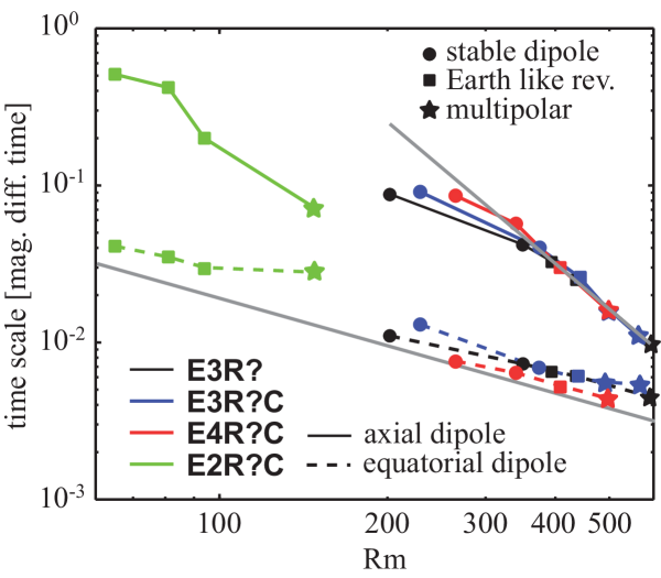
Figure 1: Dependence of typical time scales for the axial (solid lines) and equatorial dipole contribution (dashed) in all the models explored here. The lower grey line illustrates the $\mbox{Rm}^{-1}$ scaling suggested by Christensen and Tilgner (2004). The upper grey line scales like $\mbox{Rm}^{-3}$, a slope purely indicated by the data. Symbol types code the reversal behaviour.

Fig. (1) provides an overview of the different models in terms of the typical dipole time scales and the reversal behaviour. Following (Hulot and Le Mouël, 1994) and (Christensen and Tilgner, 2004) we define the time scale of a specific rms magnetic field contribution $B_{\ell m}$ by

$$t_{\ell m}=\left(\frac{\overline{{B}^{2}_{\ell m}}}{\overline{\left(B_{\ell m}(t+\delta t)-B_{\ell m}(t)\right)^{2}/\delta t^{2}}}\right)^{1/2}\;\;$$ (9)

where the overline stands for the time average. The time scales $t_{10}$ and $t_{11}$ of the axial and equatorial dipole both decrease with increasing Rayleigh number. The former, however, is typically an order of magnitude larger than the latter. Christensen and Tilgner (2004) and Lhuillier et al. (2011) report that the time scale for higher multipoles $\ell>1$ is inversely proportional to the spherical harmonic degree and also the magnetic Reynolds number,

$$t_{\ell}\sim(\ell\mbox{Rm})^{-1}\;\;,$$ (10)

while the dipole contribution has a significantly slower time scale. Fig. (1) demonstrates that this is mainly a consequence of the slow axial dipole variations (solid lines) while the equatorial dipole contribution (dashed lines) roughly agrees with the time scale $t_{1}$ suggested by eqn. (10) (lower grey line). When increasing the Rayleigh number and thus Rm, the axial dipole progressively looses its stability. Being very stable at low Ra (circles in fig. (1)), it starts to show Earth-like rare reversals when Ra is sufficiently high (squares) and ultimately enters a multipolar regime where the axial dipolar looses its dominance and reverses more or less continuously (stars). Somewhat arbitrarily, we regard reversals as Earth-like when the relative transitional time ${\tau}_{T}$ the magnetic pole spends between plus and minus $45^{\circ}$ latitude is not larger than $0.15$ and the mean dipolarity D_ℓ≤11 exceeds $0.3$. Similar but slightly stricter definitions have been used by Wicht (2005) and Wicht et al. (2011).

Once reversals have started, the time scale of the axial dipole $\tau_{10}$ decreases rapidly with a slope close to $\mbox{Rm}^{-3}$, as is demonstrated in fig. (1), and thus progressively approaches the faster time scale of the equatorial dipole and higher multipole contributions. This further confirms that the axial dipole looses its special role in strongly driven systems. Models E2R?C have not only a particularly large Ekman number but also a much smaller magnetic Reynolds number than the other cases. Fig. (1) indicates that this results in a very different behaviour. The dynamo can already reverse very close to the onset of dynamo action but with a very different type of reversals than at smaller Ekman numbers, as we will further discuss below. Another difference is that the local Rossby number already significantly exceeds the critical value $\mbox{Ro}_{\ell}\approx 0.1$ around which reversals can be expected.

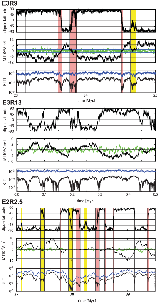
Figure 2: Examples for the evolution of different field characteristics in three dipole models. Upper sub-panels show the dipole tilt, middle sub-panels show axial dipole moment (black) and real equatorial dipole moment (green), and the lower sub-panels show the rms field strength at the CMB due to the axial dipole moment (black) and due to higher harmonic contributions $\ell>1$. Thick grey horizontal lines in the middle sub-panels show estimates for the mean axial dipole moment of the high dipole moment state while the horizontal blue lines show (eye-ball) estimates for the mean ADM in a lower dipole moment state. For the Earth-like reversing model we have indicated transitional periods with $\theta>45$ with red and yellow background colours for reversals and excursion, respectively.

Fig. (2) illustrates the temporal evolution for three selected models. The top sub-panel for each model depicts the dipole latitude $\theta=\arctan{(B_{11}/B_{10})}$ given in degree. Middle panels show axial dipole moment (AMD) and the real equatorial dipole moment (EDM). Since there is no preferred longitude in our models both the real and imaginary (or $\sin$ and $\cos$) contributions of the equatorial dipole are interchangeable and show exactly the same (statistical) behaviour. This would be different if the longitudinal symmetry would be broken by, for example, imposing a non-axisymmetric heat flux at the outer boundary condition. Vertical coloured background stripes in fig. (2) mark periods during which the dipole tilt angle $\Theta=90^{\circ}-|\theta|$ exceeds $45^{\circ}$, reversals in red and excursions in yellow. Following Wicht et al. (2009) we neglect any events shorter than $2\,$kyr and melt events closer together than $40\,$kyr to form one longer lasting event. The melting takes into account that it requires some time to reestablish the stable polarity epoches that separate individual events. When the stable polarity epochs before and after an event have the same polarity, the event is classified as an excursion rather than a reversal. We also distinguish a particular subset of excursions where the dipole ventures into the opposite polarity. These deeper ’grand excursions’ are more likely to be detected globally in paleomagnetic records (Wicht et al., 2009). The last three columns in table 1 list the number of reversals $N_{R\theta}$, grand excursions $N_{E\theta}$, and excursions $N_{e\theta}$ detected in each of the dynamo runs. We will for simplicity refer to this set of conditions as the tilt criterion in the following and mark respective quantities with the subscript $\theta$.

The axial dipole moment changes on many different time scales and shows a very complex behaviour. In the Earth-like reversing model E3R9 shown in fig. (2) we can distinguish a high dipole moment state HDM and a low dipole moment state LDM. As will be explained below, the mean ADM in the high dipole moment state $\overline{M}_{H10}=7.1\times 10^{22}$Am² can be estimated based on the statistics (thick grey horizontal line) while the LDM mean $\overline{M}_{L10}=1.7\times 10^{22}$Am² (horizontal blue line) is merely a tentative suggestion. During reversals and the longer lasting deeper excursions, the ADM tends to remain in the LDM state for some time before switching back to the HDM configuration. These events are thus not simple transitional between two states of opposite polarity but involve a new weak dipole moment state. Though a closer inspection of the ADM variation reveals more complex details, the two state description seems appropriate for characterizing the reversal behaviour, as will be demonstrated below. The equatorial dipole moment contributions show a much simpler variation around a zero mean with on average shorter time scales (see middle panels in fig. (2), green lines).

At lower Rayleigh numbers before the onset of any reversals (not shown), ADM and EDM variations show similar behaviour but the ADM simply oscillates around a larger mean of one sign and the LDM state is missing. As Ra is increased beyond the transition to the multipolar regime, reversals and excursions become much more frequent and a separation between individual events or HDM and LDM becomes difficult, as is illustrated with model E3R13 in fig. (2). The ADM is significantly weaker so that the dipole has lost its dominance and the magnetic field appears to be multipolar or complex. ADM variations still clearly show longer time scales than the EDM contributions though the difference is not as pronounced as in E3R9 (see fig. (1)).

The lower sub-panel for model E3R9 in fig. (2) reveals a high degree of correlation between the total rms dipole field and the dipole tilt angle. The correlation between the multipole field contribution and larger tilt angles is still detectable but much weaker. Table 2 list various correlation coefficients for all dynamo models. For mild Rayleigh numbers where dipole tilts remain generally small, the tilt variations are mainly caused by equatorial dipole variations as attested by the high correlation coefficients $\mathcal{C}(\mbox{B}_{11},\Theta)\geq 0.8$. When the Rayleigh number is increased, axial dipole fluctuations start to play a more important role and the respective correlation coefficient $\mathcal{C}(\mbox{B}_{10},\Theta)$ increases up to $0.7$ for reversing models while $\mathcal{C}(\mbox{B}_{11},\Theta)$ decreases. Large tilt angles are generally caused by a decreasing axial dipole contribution. The smaller but still significant correlation between tilt angle and higher multipoles is a consequence of the high correlation between axial dipole and multipole contributions $\mathcal{C}(\mbox{B}_{10},\mbox{B}_{\ell>0})$ which typically exceeds $0.8$. The high value reflects the coupling of different scales via the dynamo process where the dipole contributions is produced from higher degree contributions and vice versa. The correlation between the equatorial dipole and higher harmonics is significantly lower likely because the equatorial dipole belongs to the less preferred equatorially symmetric dynamo family. In the multipolar regime, $\mathcal{C}(\mbox{B}_{10},\mbox{B}_{\ell>0})$ decreases while $\mathcal{C}(\mbox{B}_{11},\mbox{B}_{\ell>0})$ remains largely unchanged, at least for the smaller Ekman number dynamos (Wicht et al., 2011). This is another indication that the axial dipole looses its special role at larger Rayleigh numbers.

Name	Revs.	$\mathcal{C}(\mbox{B}_{10},\Theta)$	$\mathcal{C}(\mbox{B}_{11},\Theta)$	$\mathcal{C}(\mbox{D${}_{\ell\leq 11}$},\Theta)$	$\mathcal{C}(\mbox{B}_{10},\mbox{B}_{\ell>0})$	$\mathcal{C}(\mbox{B}_{11},\mbox{B}_{\ell>0})$
E3R5	-	$0.05$	$0.96$	$0.08$	$0.72$	$0.26$
E3R7	-	$-0.20$	$0.85$	$-0.15$	$0.83$	$0.30$
E3R8	E	$-0.51$	$0.48$	$-0.54$	$0.85$	$0.32$
E3R9	E	$-0.62$	$0.39$	$-0.61$	$0.83$	$0.34$
E3R13	M	$-0.71$	$0.43$	$-0.53$	$0.53$	$0.33$
E3R9C	-	$-0.11$	$0.98$	$0.03$	$0.55$	$0.15$
E3R19C	-	$-0.13$	$0.75$	$-0.14$	$0.87$	$0.47$
E3R23C	E	$-0.61$	$0.28$	$-0.62$	$0.86$	$0.42$
E3R28C	M	$-0.68$	$0.37$	$-0.58$	$0.71$	$0.37$
E3R38C	M	$-0.72$	$0.44$	$-0.46$	$0.48$	$0.40$
E4R53C	-	$-0.09$	$0.97$	$-0.07$	$0.77$	$0.15$
E4R78C	-	$-0.35$	$0.64$	$-0.47$	$0.88$	$0.31$
E4R106C	E	$-0.63$	$0.20$	$-0.70$	$0.87$	$0.39$
E4R159C	M	$-0.68$	$0.33$	$-0.66$	$0.70$	$0.34$
E2R1.8	-	$-0.02$	$0.80$	$0.09$	$0.83$	$0.10$
E2R2.2	E	$-0.45$	$-0.17$	$-0.63$	$0.97$	$0.73$
E2R2.5	E	$-0.59$	$0.13$	$-0.65$	$0.88$	$0.46$
E2R4.2	M	$-0.61$	$0.24$	$-0.42$	$0.80$	$0.57$

Table 2: Correlation coefficients between various rms field contributions, the tilt angle $\theta$, and the dipolarity D_ℓ≤11.

The other two lower Ekman number setups E3R?C and E4R?C show very similar behavior but setup E2R? is clearly different. Fig. (2) demonstrates that the dynamo stops operating intermittently in model E2R2.5 so that all field components decay and only slowly recover some time later. The axial dipole may still dominate during these epochs and undergo stochastic reversals and excursions. However, the total field can assume a rather low level and the dipole remains relatively unstable even in the inter-event periods. We will refer to these special events as reversals and excursions of type 2 to distinguish them from the more typical events of type 1 which predominantly concern variations in the axial dipole component. Model E2R2.5 shows reversals of both types while the smaller Ra in models E2R1.8 and E2R2.2 allows only for reversals of type 2. Another difference between the large and the lower Ekman number models is that the Earth-like reversing case E2R2.5 shows more reversals than excursions (see table 1).

4 A Gaussian reversal model

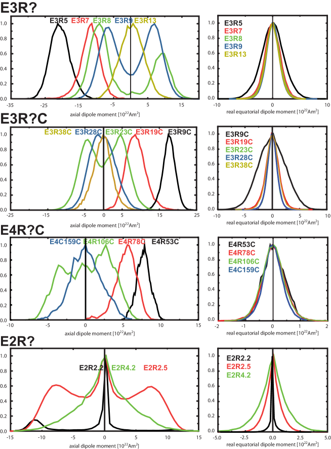
Figure 3: Rayleigh number dependence of axial dipole moment histograms (left) and real equatorial dipole moment histograms (right) for all explored models. All histograms have been normalized with the respective maximum.

Fig. (3) shows how the histograms of axial and real equatorial dipole moment change with Rayleigh number in the different model setups. We start with discussing the rather similar properties in models E3R?, E3R?C, and E4C. The ADM assumes a rather simple Gaussian shape for smaller Rayleigh numbers. On increasing Ra the histogram retains its overall shape while the (absolute) mean decreases. Reversals start once low dipole moments become more likely and the histogram then assumes a bimodal shape with ADM values of both signs. However, the low ADM states are more populated than a superposition of two symmetric Gaussians would imply. The relative likelihood of low values further increases with Ra until the distribution looks like a Gaussian with zero mean in the multipolar regime.

While fig. (2) seemed to indicate that the low ADM state may also consist of two symmetric distributions this is not supported by the AMD histograms. However, the superposition of the two Gaussians may simply be indistinguishable from a distribution with zero mean and larger standard deviation. Similarly, the two high ADM states may still contribute to the flanks of the distribution in the multipolar regime. The EDM histograms in the lower Ekman number cases remain surprisingly similar for all Rayleigh numbers and always assume a Gaussian shape with zero mean (see fig. (3), right column).

Several authors have suggested that the geomagnetic field actually obeys a Gaussian model with a non-zero mean for the axial dipole and zero means for all other field coefficients (Constable and Parker, 1988; Hulot and Le Mouël, 1994). Our simulations suggest that this model oversimplifies the axial dipole distribution. The required correction, however, is likely only small and concerns only data covering a fair portion of transitional epochs.

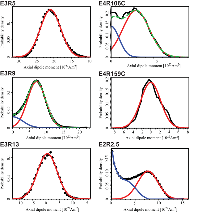
Figure 4: Fit of Gauss distributions to some of the ADM histograms. For the reversing models E3R9 and E4R106C the red and blue lines show the Gauss distributions for the high and low dipole moment states, respectively. For case E2R2.5 the blue curve is the difference between the numerical distribution and the red Gauss distribution which was fitted to the right flank of the numerical distribution.

We have tried to fit Gaussian distributions to the ADM and the EDM components in all models, using a least-squares procedure for the binned data. The respective results are illustrated for a few selected cases in fig. (4). To disentangle the HDM and LDM contributions in the Earth-like reversing cases we analyse the unsigned dipole moment, assuming that the distributions should be symmetric around zero. The HDM axial dipole Gaussian is then fitted to the right flank of the unsigned ADM distribution beyond the distribution maximum. The LDM Gaussian is fitted in a second step after subtracting the HDM model. The Gaussians convincingly reproduce the ADM and EDM distributions for models E3R? and E3R?C. The histograms are less smooth for the shorter runs of E4R?C but the model distributions nevertheless seem to provide a fair representation, as is demonstrated in fig. (4).

The histograms for E2R? clearly deviate from the Gaussian models and reflect the intermittent nature of the dynamo process in the form of pronounced peaks around zero. Here we only fitted the HDM part of the axial dipole moment. The peaked equatorial dipole moment, LDM axial dipole moment, and multipolar axial dipole moment distributions are far from a normal distribution.

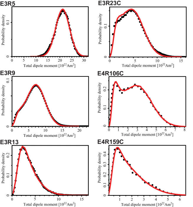
Figure 5: Histograms of the total dipole moment in different dynamo models. Black dots show the numerical simulation data while red lines are the predictions based on drawing random samples from the axial and equatorial dipole moment distributions.

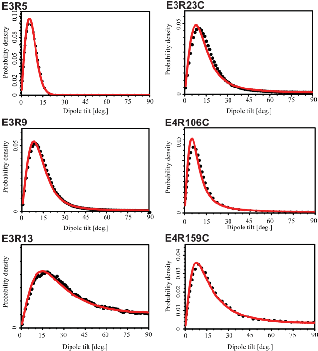
Figure 6: Histograms of the dipole tilt angle in different dynamo models. Black dots show the numerical simulation data while red lines are the predictions based on the Gaussian models.

The correlation coefficients between all three dipole contributions never exceed a few percent so that they are likely statistically independent. This suggests that the total dipole moment $M$ and the dipole tilt $\theta$ can be predicted by combining randomly and independently drawn samples from the individual moment distributions. The procedure indeed produces convincing representations of the respective numerical distributions as is demonstrated for a few examples in fig. (5) and fig. (6). The procedure works best for the longer runs E3R? and somewhat less convincingly for E3R?C and E4R?C. We did not attempt predictions for the larger Ekman number models E2E? because of their complex non-Gaussian histograms.

Table 3 list mean and standard deviations for the different Gaussian distributions describing the dipole moment histograms. For the smaller Ekman number cases the total dipole moment in the HDM state can be approximated by the respective axial dipole moment distribution. For estimating the total dipole moment distribution in the LDM state, we used randomly drawn samples from the respective axial and equatorial dipole distributions to first estimate the dipole energy distribution which closely resembles the expected $\chi^{2}$ distribution for three independent variables (Hulot and Le Mouël, 1994). From this we calculated the mean $\overline{M}_{L}$ and its standard deviation listed in table 3. Earth values given in table 3 are only very rough estimates based on data covering the last $2\,$Myr by Valet et al. (2005) and Channell et al. (2009). Note, however, that the recent dipole moment estimates by Ziegler et al. (2011) yield significantly lower dipole moment amplitudes.

Knowing mean and standard deviation $\sigma$ of the individual Gaussian distributions is apparently sufficient to predict the dipole moment and tilt probability for the lower Ekman number simulations with some confidence. The respective values are listed in table 3 for the reversing dynamo models that we will further explore below. Since the two equatorial dipole moments behave identically we have to specify only two distributions for non-reversing and three for reversing dynamos. When taking into account that equatorial moment and LDM distributions have a zero mean, the total dipole moment and tilt predictions rely on only three parameters for non reversing dipolar dynamos ($\overline{M}_{10}$,$\sigma(M_{10})$,$\sigma(M_{11})$), on four parameters for reversing dynamo ($\overline{M}_{H10}$,$\sigma(M_{H10})$,$\sigma(M_{L10})$,$\sigma(M_{11})$), and on two parameters for multipolar dynamos ($\sigma(M_{10})$,$\sigma(M_{11})$). Indices refer to high (H) or low (L) dipole moment states and axial (10) or equatorial (11) contributions.

Model	$\overline{M}$	$\sigma(M)$	$\overline{M}_{H10}$	$\sigma(M_{H10})$	$\overline{M}_{L10}$	$\sigma(M_{L10})$	$\overline{M}_{11R}$	$\sigma(M_{11R})$	$\overline{M}_{L}$	$\sigma(M_{L})$
E3R9	$6.6$	$2.9$	$7.1$	$2.7$	$0.0$	$3.0$	$0.0$	$1.3$	$3.1$	$1.6$
E3R23C	$4.6$	$2.4$	$4.8$	$2.4$	$0.0$	$2.2$	$0.0$	$0.84$	$2.2$	$1.2$
E4R106C	$2.8$	$1.6$	$2.9$	$1.5$	$0.0$	$0.94$	$0.0$	$0.34$	$0.92$	$0.50$
E2R2.5	$5.3$	$3.2$	$7.7$	$2.1$	$0.0$	$2.8$	$0.0$	$0.78$	-	-
Earth	$7$	-	$9$	$3$	-	-	-	-	$2$	-

Table 3: Mean and standard deviation of the total dipole moment $M$ and the individual dipole moment contributions in the high dipole moment (H) and low dipole moment (L) states. Suffix $10$ and $11R$ indicate the axial contribution and the real part of the equatorial contributions, respectively. High and low state values refer to the fitted Gaussian distributions. The high state total moment $\overline{M}_{H}$ is very similar to $\overline{M}_{H10}$ and is therefore not listed. The low state total moment $\overline{M}_{L}$ has been estimated by combining randomly drawn samples from the distributions of ${M}_{L10}$ and ${M}_{11R}$.

5 Reversals, a process in three stages

The two-state scenario outlined above suggests that reversals can be separated into three stages. The first stage is the decay of the axial dipole moment until the LDM state is reached. Total dipole moment $M$ or mean field strength also clearly drop since the axial dipole dominates initially. The period spent in the LDM state defines the second stage during which ADM variations cause one or several polarity changes until the axial dipole moment grows enough to re-establish the HDM state in the final third stage. Since the number of polarity switches during stage two seems to be stochastic it is simply a matter of chance which axial dipole direction is amplified in stage three. There should thus be a class of grand excursions which shares the statistical properties of reversals. To explore this idea we refine our definition of grand excursions, requiring not only that the dipole ventures into opposite polarity but also assumes amplitudes typical for the LDM state.

To verify and further explore the three-stage model we integrated four Earth-like reversing models long enough to provide some statistics of the complex and highly variable processes (see table 1). For defining the stages we rely on the total rather than only the axial dipole moment since only the former is reasonably accessible for palaeomagnetic studies. The reversals and excursions detected with the tilt criterion serve as a first guess for determining the start of each event $t_{s}$ and its end $t_{e}$ when the DM decreases below or exceeds a threshold $M_{Hc}$. The event duration including all three stages is then given by $t_{V}=t_{e}-t_{s}$. To determine the decay and growth rate in stage one and three we assume that the decay ends at $t_{De}$ when the DM decreases below a second threshold $M_{Lc}$ and the growth stage starts at $t_{Gs}$ once $M_{Lc}$ is once more exceeded. The decay and growth time scales ${\tau}_{D}$ and ${\tau}_{G}$ are then expressed in fractions of the dipole decay time by comparing $e$-folding times:

$${\tau}_{D}=\frac{t_{De}-t_{s}}{T_{D}}\,\frac{M_{Hc}(1-1/e}{M_{Hc}-M_{Lc}}=\frac{t_{D}}{t_{d}}\;\;,$$ (11)

$${\tau}_{G}=\frac{t_{e}-t_{Gs}}{T_{D}}\,\frac{M_{Hc}(1-1/e}{M_{Hc}-M_{Lc}}=\frac{t_{G}}{t_{d}}\;\;.$$ (12)

The time spent in the LDM state can be estimated by $t_{L}=t_{Gs}-t_{De}$. We will also briefly discuss the waiting time between events $t_{W}=t_{s}^{(n)}-t_{e}^{(n-1)}$ where the upper index refers to the event number.

To exclude the influence of statistical shorter term fluctuations we have used a running mean of the dipole moment with a window of $5\,$kyr or $0.1$ dipole decay times. This is about five times the flow overturn time in the reversing simulations. Experiments show that windows of a few thousand years provided the most consistent timing of reversals and excursions. Overlapping consecutive events are simply dismissed which generally reduces the number of reversals $N_{R}$ and grand excursions $N_{E}$ entering the analysis.

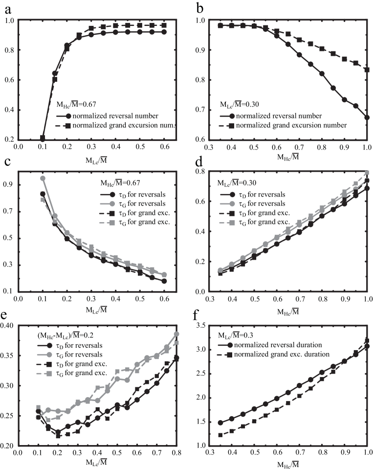
Figure 7: Dependence of the number of reversals and grand excursions (a and b) and the time scales $\tau_{D}$ and $\tau_{G}$ (c, d) in model E3R9 on $M_{Hc}$ and $M_{Lc}$ when the respective other parameter is held fixed. The event number has been normalized with the event number based in the tilt criterion alone. Panel e illustrates the dependence of $\tau_{D}$ and $\tau_{G}$ on $M_{Lc}$ for a constant difference $M_{Hc}-M_{Lc}$. Panel f shows the dependence of the event durations on $M_{Hc}$.

How should the thresholds $M_{Hc}$ and $M_{Lc}$ be chosen? The mean of the HDM state minus its standard deviation seems a natural first guess for $M_{Hc}$. Since the ADM is much larger than the EDM we can for simplicity use the ADM mean and standard deviation: $M_{Hc}=\overline{M}_{H10}-\sigma(M_{H10})$. Choosing $M_{Lc}=\overline{M}_{L}$ seems a reasonable first guess for the lower threshold. For model E3R9 the above reasoning suggests $M_{Hc}=4.4\mbox{$\times 10^{22}$}$Am² and $M_{Lc}=3.1\times{22}$Am². In the following a calligraphic ${\mathcal{M}}$ will refer to dipole moments normalized with the time averaged mean. The E3R9 threshold estimates are then ${\mathcal{M}}_{Hc}=0.67$ and ${\mathcal{M}}_{Lc}=0.47$ respectively.

To understand the role of the thresholds we have explored their impact on the different reversal and excursion properties. Fig. (7) illustrates how the event number and time scales depend on the choice of ${\mathcal{M}}_{Hc}$ and ${\mathcal{M}}_{Lc}$ for model E3R9. Panel a reveals that the dipole moment has to decrease to a critical value of about $30$% of its mean to facilitate reversals and grand excursions. For lower values we start losing events where the running mean never decays as much. If, on the other hand, ${\mathcal{M}}_{Hc}$ exceeds about $0.65$ we disregard stable polarity intervals during which the dipole moment never exceeds the threshold (see fig. (7)b). Considering values outside the interval $(0.30-0.65)$ would thus potentially distort the statistics. Naturally, missing events have a particularly large effect on the event waiting times (or inter-event times) as will be illustrated below.

Ruling out the statistical short term variations around the high and low dipole moment states seems essential for estimating the decay and grow time scales ${\tau}_{D}$ and ${\tau}_{G}$. This is not an easy task since dipole moment variations are generally complex and the distributions of HDM and LDM states overlap. Considering the $5\,$kyr running mean only partially solves this problem and the event timing remains very sensitive to the threshold values as is demonstrated in the lower four panels of fig. (7). Asymptotical values of ${\tau}_{D}$ and ${\tau}_{G}$ are only approached when ${\mathcal{M}}_{Lc}$ and ${\mathcal{M}}_{Hc}$ become very similar. The timescales then characterize a rather brief episode more typical for the faster statistical variations than the slower longer term transition from the high to the low dipole moment state.

Fig. (8) further illustrates the problem of selecting appropriate thresholds. When ${\mathcal{M}}_{Hc}$ is too large, short term variations before or after the decisive transition are regarded as part of the decay or growth period which leads to longer time scale estimates (compare blue and green line for the growth period in fig. (8)). Similar reasoning holds when ${\mathcal{M}}_{Lc}$ is too low (green and yellow line for the growth period in fig. (8)). This suggest that the total decay $\Delta{\mathcal{M}}={\mathcal{M}}_{Hc}-{\mathcal{M}}_{Lc}$ is a key parameter and the nearly linear dependence on ${\mathcal{M}}_{Hc}$ indicates that ${\tau}_{D}$ and ${\tau}_{G}$ could be roughly proportional to $\Delta{\mathcal{M}}$. Fig. (7)e indeed demonstrates that the time scales are less sensitive to ${\mathcal{M}}_{Hc}$ or ${\mathcal{M}}_{Lc}$ once $\Delta{\mathcal{M}}$ is kept fixed. However, the variation still remains significant and the time to change the dipole moment by a fixed percentage increases with the dipole moment. The absolute rather than the relative change is therefore also relevant. Panel f of figure fig. (7) shows the dependence of the total mean event durations $\overline{{\tau}_{V}}$, normalized with the dipole decay time, on the threshold ${\mathcal{M}}_{Hc}$. Durations of up to three dipole decay times seem possible which would correspond to roughly $150\,$kyr for Earth.

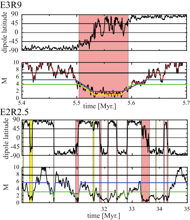
Figure 8: Dipole tilt and dipole moment variations during selected periods in model E3R9 (top) and E2R2.5 (bottom). The red line in the second panel shows the $5\,$kyr running mean while the other coloured lines illustrate estimates for the decay and growth periods. Horizontal parts show the threshold dipole moments while the tilted parts mark the transitions between the assumed high and low dipole moment states. Model E3R9: blue line for ${\mathcal{M}}_{Hc}=M_{Hc}/\overline{M}=0.8$ and green line for ${\mathcal{M}}_{Hc}=0.6$, both using ${\mathcal{M}}_{Lc}=M_{Lc}/\overline{M}=0.3$. The yellow line illustrates the combination (${\mathcal{M}}_{Hc}=0.60$,${\mathcal{M}}_{Lc}=0.15$). Model E2R2.5: blue line for (${\mathcal{M}}_{Hc}=1.1$,${\mathcal{M}}_{Lc}=0.5$) and green line for (${\mathcal{M}}_{Hc}=0.6$,${\mathcal{M}}_{Lc}=0.3$). Yellow and red background stripes once more show the excursions and reversals identified with the tilt criterion. Thick horizontal black lines in dipole moment panels show the mean value $\overline{M}_{H}$ of the high dipole moment state.

Fig. (7) also illustrates that some properties remain independent of the thresholds: a) the growth is on average only about $10$% slower than the decay, b) both processes are faster than the dipole decay time ($\tau$ smaller than one), c) grand excursions and reversals have very similar characteristics, and d) the dipole moment has to decrease to about $30$% of its mean value to allow for reversals and grand excursions.

The combination ${\mathcal{M}}_{Lc}=0.30$ and ${\mathcal{M}}_{Hc}=0.60$, somewhat smaller than the values suggested by the Gaussian model, seems to offer an acceptable compromise for E3R9 that we adopt for further analysis. Reasonable mean values for the decay and growth time scales roughly range from $\overline{{\tau}}=0.20$ to $\overline{{\tau}}=0.40$ while mean event durations range from $\overline{{\tau}_{V}}=1.5$ to $\overline{{\tau}_{V}}=2.0$. The analogous analysis for the reversing models E3R23C and E4R106C yields very similar results. Decay and growth time scales are even more similar than for model E3R9. Both scales are about $25$% smaller in model E4R103C than in models E3R9 and E3R23C.

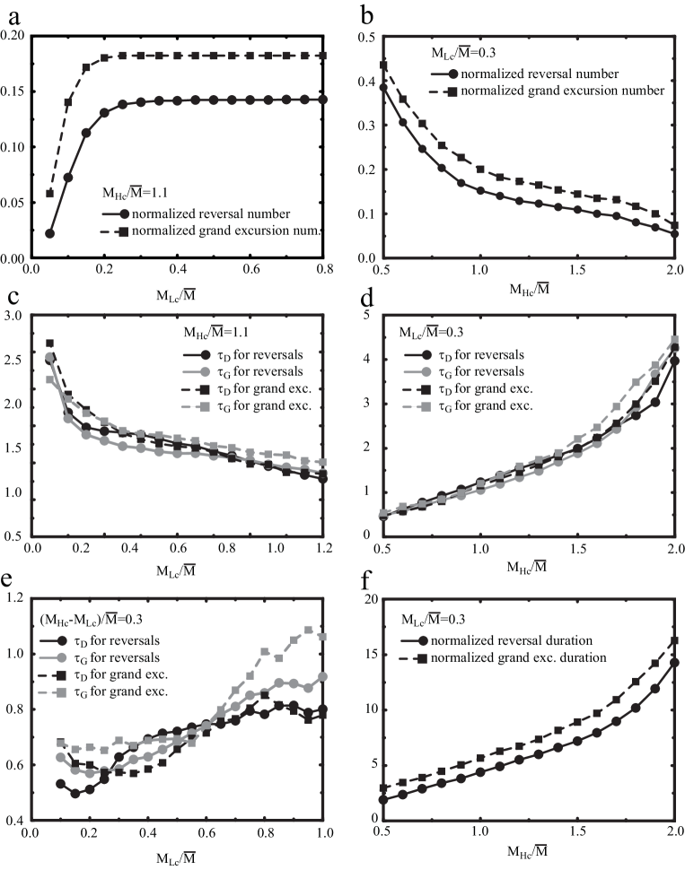
Figure 9: Same as fig. (7) but for model E2R2.5.

Not surprisingly, the different characteristic of the large Ekman number models is also reflected in the reversal and grand excursion timing. The analysis of the dipole moment distribution yields a mean high dipole moment state of $\overline{M}_{H}=1.5\overline{M}$ for E2R2.5 and a standard deviation of $\sigma(M)=0.4\overline{M}$. This suggest an upper threshold of ${\mathcal{M}}_{Hc}=1.1$ which, however, significantly reduces the event number as is demonstrated in fig. (9)b. The peak in the axial dipole moment distribution that served for defining $\overline{M}_{H}$ has obviously little to do with the majority of reversals and excursions. The statistics only recovers to some degree when choosing significantly lower values comparable to those used in the other models. For ${\mathcal{M}}_{Hc}=0.6$ and ${\mathcal{M}}_{Lc}=0.3$, the values we adopt for further analysis, about 40% of the reversals and grand excursions identified by the tilt criterion enter the time scale analysis. The lower panels in fig. (8) further illustrate the difficulties in choosing appropriate threshold values for E2R2.5. From the 9 reversals identified with the tilt criterion only one remains for the high threshold value of ${\mathcal{M}}_{Hc}=1.1$ (blue line) while four are retained for ${\mathcal{M}}_{Hc}=0.6$ (green line). Many reversals and excursions happen during episodes of low dipole field strength and relatively unstable tilt angles which complicates the clear timing and separation of events.

Fig. (9) demonstrates that the dependence of the time scales on ${\mathcal{M}}_{Hc}$ and ${\mathcal{M}}_{Lc}$ is nevertheless similar to those found for the other models. Once more reversals and grand excursions show comparable characteristics but take significantly longer than in the smaller Ekman number cases. $\overline{{\tau}_{D}}$ and $\overline{{\tau}_{G}}$ now range between $0.5$ and $2.0$ which seems to suggest that a stop in dynamo action and the subsequent magnetic field decay may play a role in the reversal process. However, since the growth time scale is also very similar, the long time scale seems to be a more general feature of this dynamo and is possibly a consequence of the low magnetic Reynolds number. Fig. (9)f demonstrates that the event durations are also particularly long, ranging from $3$ to $15$ dipole decay times. The longer estimates are characteristic for larger values of ${\mathcal{M}}_{Hc}$ where reversals and grand excursions during weaker field periods are not taken into account.

6 Time scale statistics

Model	${\mathcal{M}}_{Hc}$	${\mathcal{M}}_{Lc}$	event	$N_{\theta}$	$N$	$\overline{t_{D}}$	$\overline{t_{G}}$	$\overline{t_{L}}$	$\overline{t_{V}}$	$\overline{t_{W}}$	$\overline{\left(\frac{{\tau}_{D}}{{\tau}_{G}}\right)}$	min$\left(\frac{{\tau}_{D}}{{\tau}_{G}}\right)$	max$\left(\frac{{\tau}_{D}}{{\tau}_{G}}\right)$
E3R9	$0.60$	$0.30$	R	$542$	$513$	$18$	$20$	$82$	$112$	$1840$	$0.88$	$0.05$	$7.2$
			E	$613$	$590$	$18$	$20$	$67$	$99$	$1808$	$0.85$	$0.06$	$12.0$
E3R23C	$0.60$	$0.35$	R	$105$	$100$	$21$	$24$	$69$	$101$	$881$	$0.89$	$0.04$	$8.3$
			E	$104$	$100$	$23$	$23$	$65$	$101$	$909$	$0.81$	$0.08$	$7.1$
E4R106C	$0.60$	$0.30$	R	$20$	$20$	$13$	$13$	$62$	$81$	$740$	$0.89$	$0.26$	$3.6$
			E	$29$	$30$	$14$	$11$	$84$	$104$	$613$	$1.20$	$0.17$	$11.1$
E2R2.5	$0.60$	$0.30$	R	$2956$	$906$	$35$	$33$	$80$	$134$	$2458$	$1.05$	$0.06$	$12.5$
			E	$948$	$340$	$33$	$39$	$140$	$197$	$2338$	$0.88$	$0.06$	$8.3$
Earth	$0.75$	$0.30$	R	–	–	$33$	$8$	–	$49$	$250$	$4$	–	–

Table 4: Properties of reversals and grand excursion (R or E in column 4) for selected parameters in the four examined Earth-like reversing models and for Earth. Column six list the reduced event number when including the dipole moment thresholds in the event definition. Columns 7 to 10 show the mean decay and growth time scales $t_{D}$ and $t_{G}$, mean time spent in the LDM state $\overline{{\tau}_{L}}$, mean event duration $\overline{{\tau}_{V}}$, and the mean event waiting time $\overline{{\tau}_{W}}$, all rescaled to kyr using the magnetic diffusion time scale. The last three columns list the mean ratio $\overline{{\tau}_{D}/{\tau}_{G}}$, its minimum and its maximum. Earth values are based on Valet et al. (2005) and Channell et al. (2009) and a mean reversal rate of four per Myr.

We proceed with more closely analysing the statistics of the different reversal and excursion time scales for selected threshold values. Table 4 lists mean time scales and mean, minimum and maximum ratio of decay to growth time while figures 10 to 13 show the probability density distributions. The event count ranges from $900$ reversals in model E2R2.5 to $20$ reversals in model E4R106C. The statistics is thus rather poor for the latter and very good for the former. Decay and growth times for reversals and grand excursions are very similar in each of the four models. The distributions show a lack of very short events simply because the transition requires some time. The minimum decay and growth time scales are in the order of a few millenia. The distributions peak between $0.2$ and $0.4$ dipole decay times and seem to show an exponential decay beyond. Naturally, the interpretation is somewhat difficult for E4R106C. Typical mean decay and growth time scales range from $11\,$kyr in model E4R106C for $39\,$kyr in model E2R2.5. Decay time scale estimates for Earth are on the slow side with $33\,$kyr while the growth is particularly fast with $8\,$kyr.

We have also analysed the ratio of decay to growth time for all events individually to determine whether the dipole may decay more slowly than it recovers. A related measure is $R=({\tau}_{D}-{\tau}_{G})/({\tau}_{D}+{\tau}_{G})$ which assumes positive values for a faster recovery and negative values for a faster decay. Though decay and growth rate can differ by more than an order of magnitude for a single event they are very similar on average. The decay time is typically 10% faster than the growth time with the exception of grand excursion in E4R106C and reversals in E2R2.5 (see table 4). Panels b of figures 10 to 13 demonstrate that the distributions roughly center around $R=0$, are relatively flat in the middle and decay towards extreme values of both signs. Earth value of $\tau_{D}/\tau_{G}\approx 4$ corresponds to $R=0.6$. When assuming values between $R=0.5$ and $R=0.7$ and an average probability of $0.5$ suggested by fig. (10) to fig. (13) the probability to find one Earth-like case in the simulations is about $10$%. However, the likelihood that five consecutive or very closely spaced reversals have this property, as suggested by Valet et al. (2005), is negligibly small.

The total event durations $\overline{t_{V}}$ are up to a factor four longer in the simulations than suggested for Earth (Valet et al., 2005), mostly because of the significant time $\overline{t_{L}}$ spend in the LDM state. ${\tau}_{L}$ distributions (panels c of figures 10 to 13) show a less pronounced lack of short durations that the distribution of decay and growth times, roughly obey an exponential distributions for short and intermediate values, and suggest a slower decreasing tail of longer events. The statistical significance of the tail is unclear since is mainly stays on the one-event level. Minimum values of $t_{L}$ are a millenia or shorter while the mean ranges from $\overline{t_{L}}=62\,$kyr for reversals in E4R106C to $\overline{t_{L}}=140\,$kyr for grand excursions in model E2R2.5. The distributions of the event durations $t_{V}$ (not shown) can be understood as a combination of the distributions of decay, growth, and $t_{L}$. The lack of short durations that is mostly stemms from the time required for decay and growth lead Lhuillier et al. (2013) to suggest a log-normal distribution. Mean durations range from $81\,$kyr for reversals in E4R106C to $197\,$kyr for grand excursions in E2R2.5 (see table 4).

The event waiting times $t_{W}$ are most affected by the event selection process and necessarily increases when dismissing events not deemed suitable for our time scale analysis. This effect is rather large for model E2R2.5 but negligible for the other three Earth-like reversing models. Mean waiting times range from $0.6\,$Myr for grand excursions in model E4R106C to $2.5\,$Myr for reversals in model E2R2.5. All distributions seem close to an exponential decay for shorter to intermediate durations in agreement with Wicht et al. (2009) and Lhuillier et al. (2013) but also suggest a heavier tail for very long intervals.

Generally, all reversal and grand excursion distributions are very similar with the exception of the waiting time distributions for model E2R2.5. This may partly be attributed to the event selection process but also reflects the fact that we already count three times more reversals than grand excursions when using the tilt criterion alone.

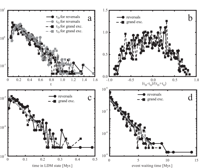
Figure 10: Distributions of time scales in model E3R9. Normalized decay and growth time scales are shown in panel a, their normalized ratio $R=({\tau}_{D}-{\tau}_{G})/({\tau}_{D}+{\tau}_{G})$ in panel b, time $t_{L}$ in the LDM state during the event in panel c and event waiting times $t_{W}$ in panel d. Tilted grey lines in panel c and d are exponential distributions that are not the product of a fitting procedure but simple eye-balled suggestions.

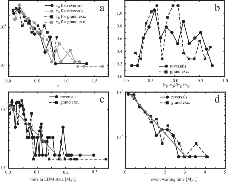
Figure 11: Same as fig. (10) but for model E3R23C.

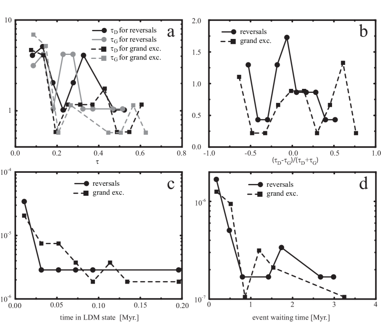
Figure 12: Same as fig. (10) but for model E4R106C.

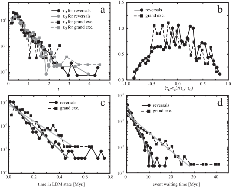
Figure 13: Same as fig. (10) but for model E2R2.5.

7 Overshoot?

The magnetic field strength clearly overshoots more normal values at the end of reversals in the VKS experiment and in some low order dynamical models (Pétrélis et al., 2009). The fast field recovery at the end of a reversals continues to amplitudes significantly above the mean value and the level of typical fluctuations. The situation is less clear for paleomagnetic reversals, however. Only two of the five record discussed by Valet et al. (2005) show an ’overshoot’ which remains within the level of other dipole moment fluctuations. In a statistical sense an ’overshoot’ then simply means that a higher field level is reached in a particularly short time.

To check whether this is the case in the numerical simulations we simply raised the thresholds to values within normal dipole moment variations and show results for the combinations $({\mathcal{M}}_{Lc}=1.0,{\mathcal{M}}_{Hc}=1.3)$ and $({\mathcal{M}}_{Lc}=1.0,{\mathcal{M}}_{Hc}=1.6)$ here. Once more both the decay and the growth time scales required to reach the respective other threshold are estimated and we restrict the analysis not only to reversals (R) and grand excursions (E) but also more generally consider all (A) dipole moment fluctuations. The respective mean time scales and time scale ratios are listed in table 5 where column four indicates the three event types. Fig. (14) compares the different time scale distributions.

Model	${\mathcal{M}}_{Lc}$	${\mathcal{M}}_{Hc}$	event	$N_{D}$	$N_{G}$	$\overline{t_{D}}$	$\overline{t_{G}}$	$\overline{\left(\frac{{\tau}_{D}}{{\tau}_{G}}\right)}$	min$\left(\frac{{\tau}_{D}}{{\tau}_{G}}\right)$	max$\left(\frac{{\tau}_{D}}{{\tau}_{G}}\right)$
E3R9	$1.0$	$1.3$	A	$6275$	$6274$	$26$	$28$	$0.90$	$0.04$	$15.5$
			R	$339$	$347$	$24$	$29$	$0.82$	$0.06$	$14.9$
			E	$462$	$485$	$25$	$28$	$0.88$	$0.07$	$11.4$
		$1.6$	A	$3205$	$3205$	$45$	$47$	$0.92$	$0.04$	$18.4$
			R	$325$	$331$	$43$	$51$	$0.82$	$0.05$	$11.0$
			E	$424$	$438$	$45$	$48$	$0.89$	$0.09$	$16.4$
E3R23C	$1.0$	$1.3$	A	$615$	$616$	$23$	$25$	$0.91$	$0.04$	$14.6$
			R	$71$	$73$	$20$	$24$	$0.85$	$0.09$	$10.1$
			E	$74$	$77$	$22$	$30$	$0.72$	$0.06$	$4.7$
		$1.6$	A	$354$	$355$	$36$	$37$	$0.92$	$0.07$	$15.0$
			R	$66$	$69$	$31$	$38$	$0.78$	$0.16$	$7.6$
			E	$67$	$71$	$39$	$36$	$0.98$	$0.13$	$7.6$
E4R106C	$1.0$	$1.3$	A	$110$	$110$	$21$	$25$	$0.82$	$0.13$	$14.4$
			R	$9$	$11$	$13$	$25$	$0.76$	$0.16$	$2.2$
			E	$16$	$21$	$16$	$29$	$0.61$	$0.09$	$3.3$
		$1.6$	A	$70$	$70$	$36$	$44$	$0.84$	$0.12$	$5.7$
			R	$9$	$10$	$38$	$47$	$0.77$	$0.16$	$4.1$
			E	$16$	$20$	$35$	$46$	$0.66$	$0.17$	$6.2$
E2R2.5	$1.0$	$1.3$	A	$4585$	$4585$	$55$	$58$	$0.94$	$0.07$	$15.3$
			R	$419$	$443$	$55$	$59$	$0.90$	$0.11$	$7.5$
			E	$180$	$188$	$47$	$65$	$0.74$	$0.10$	$4.2$
	$1.0$	$1.6$	A	$3445$	$3445$	$79$	$88$	$0.87$	$0.02$	$12.4$
			R	$411$	$435$	$80$	$92$	$0.85$	$0.06$	$7.8$
			E	$175$	$185$	$68$	$89$	$0.74$	$0.10$	$8.0$

Table 5: Properties of decay (index D) and growth (index G) time scales for reversals, grand excursion and all dipole moment fluctuations (R, E, or A in column four) for selected parameters in the four examined Earth-like reversing models. Columns five and six list the event counts, columns seven and eight the time scales in kyr and columns 9 to 11 the mean, minimum and maximum ratio of decay and consecutive growth time for individual events.

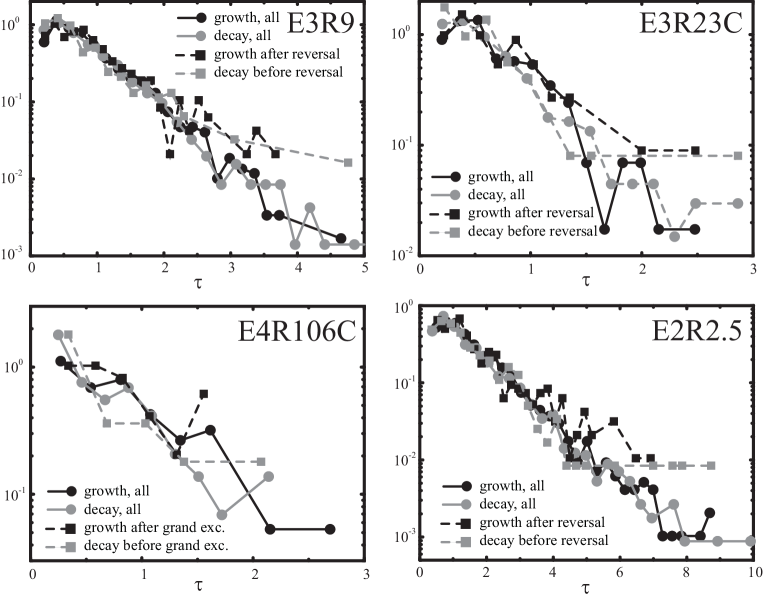
Figure 14: Time scale distributions for the four analysed Earth-like reversing models and thresholds ${\mathcal{M}}_{Hc}=1.6$ and ${\mathcal{M}}_{Lc}=1$. The individual panels compare all dipole moment variations with those before and after reversals (models E3R9, E3R23C, E2R2.5) or grand excursions (mode E4R106C).

The time scales for all three event types are very similar so that the variations leading in and out of reversals and grand excursions are nothing special. There is no indication for any overshoot behaviour. The properties are also similar to the decay and growth from the HDM to the LDM state discussed in section 5. Time scale values below $\tau=1$ once more indicate active dynamo processes rather than dipole decay. Distributions lack short events because of the limited time required to amplify dipole field of normal or reversed polarity. A pair of decay and following growth time can once more differ greatly and the decay is on average somewhat faster. The mean ratio of decay to growth times reaches lower values than for the HDM-LDM transition. The smallest ratio of $0.61$ for grand excursion in model $E4R106C$, however, is based on rather poor statistics and a $10$ to $20$% faster decay seems more typical.

A comparison of time scales for $({\mathcal{M}}_{Hc}=1.3,{\mathcal{M}}_{Lc}=1)$ in table 5 and ${\mathcal{M}}_{Hc}=0.6,{\mathcal{M}}_{Lc}=0.3)$ in table 4 confirms that the time required to change the mean dipole moment by $30$% increases with the amplitude of the dipole moment (see also panels e in fig. (7) and fig. (9).

8 Discussion

The analysis of dipole moment fluctuations in extremely long dynamo simulations reveals some interesting properties of reversals and excursions. At low Rayleigh numbers, the axial dipole moment distribution assumes a Gaussian shape with a non zero mean as suggested by Giant Gaussian models (Constable and Parker, 1988; Hulot and Le Mouël, 1994). The mean decreases with growing Rayleigh number until at some point very low dipole moments become more likely. The dynamo can then switch from the high dipole moment state to a new weak field state which is characterized by the fact that the axial dipole moment assumes a Gaussian distribution with zero mean, behaves largely like the higher harmonic field contributions, and frequently switches polarity.

When the dynamo recovers from the weak to the high dipole moment state, the axial dipole direction is just a matter of chance. Reversals and grand excursions are therefore equally likely and have virtually identical properties. Grand excursions are excursions during which the dipole moment assumes values typical for the low dipole moment state. Other excursions still feature large or even inverse tilt angles, in particular when local magnetic field data are considered (virtual dipole moment) (Wicht et al., 2009), but never a full polarity switch. The simulations suggest that a drop to $30$% of the mean field strength is required to allow for reversals or grand excursions. This is very similar to the values estimated from paleomagnetic data.

The simulated reversals are thus likely initiated by particularly large variations in the dipole moment and not necessarily by any special internal event. The event remain rare since the variations have to reach the ’outer weak dipole flank’ of the Gaussian distribution. Similar scenarios are discussed in low-order dynamical models geared to explain the reversals in the VKS experiment (Pétrélis et al., 2009), but there are important differences. Larger variations that lead beyond the unstable point in the low-order models are followed by a faster recovery of the dipole moment with opposite polarity and by an overshoot. In the numerical simulations, the larger variations leads to the weak dipole state and since the system tends to linger in this state for some time it cannot be considered as unstable in the sense of the low-order models. Consequently, the numerical simulations neither show a faster recovery not an overshoot. Both features have been suggested by some paleomagnetic studies (Valet et al., 2005) but are not firmly established.

On average the field decay happens about $10$% faster than the growth not only related to reversals and grand excursions but also for larger amplitude dipole moment variations in general. Paleomagnetic estimates predict a four times faster growth rate for reversals and $20$% faster growth rate for general dipole moment fluctuation.

Even though there is no significant asymmetry in decay and growth the time scales for these two phases are nevertheless similar to those suggested for Earth (Valet et al., 2005; Ziegler and Constable, 2011). The overall longer duration of the simulated reversals and excursions is mostly caused by the pronounced time spent in the lower dipole moment state. Some paleomagnetic records tend to show a similar lingering at low field intensities though not to the same extend. The Cobb Mountain event is a prime example (Channell et al., 2009), the upper Olduvai or even the Matuyama-Brunhes transitions are other possible candidates where the field seem to vary around a lower value for some time (Valet et al., 2005; Lund et al., 2006; Ziegler et al., 2011).

In terms of a low-dimensional dynamical system reversals and grand excursions are best described by the three attractors or states suggested by Lhuillier et al. (2013), two are the high dipole moment states of both polarities and the third is the low dipole moment state that connects both. The relative stability of these states depends on the system parameters. For Earth-like reversals, the low dipole state is considerably less stable than the high dipole state. However, this changes at larger Rayleigh numbers where the low dipole state seems to be preferred in the multipolar regime. Other system parameters like the outer boundary heat flux pattern (Glatzmaier et al., 1999; Kutzner and Christensen, 2004; Olson et al., 2010, 2013) or the inner thermal boundary conditions (Dharmaraj and Stanley, 2012) are also known to have an impact on the reversal behaviour. The reversal and grand excursion properties are comparable for the three smaller Ekman number models explored here. However, the rate of reversals and grand excursion is about two times lower for the thermally driven dynamo E3R9 than for the compositionally driven dynamo E3R23C, despite the fact that magnetic Reynolds number, local Rossby number and other system characteristics are very similar.

During the reversals of type 1 described above only the axial dipole moment decreases while the other field contributions remain largely unaffected. The larger Ekman number models with $E=2\mbox{$\times 10^{-2}$}$ show a second type of reversals of type 2 where the total field decays for a some time and then recovers. Common to both types is that reversals and grand excursions are only possible when the field is low while other characteristics are rather different. Type 2 reversals likely play no role for Earth where at least the multipolar components remain sizable during the events.

The simulations have confirmed that dipole moment variations are complex and happen on many different time scales. Reversals and excursions are therefore highly variable and a statistical approach is required to access their properties. This became possible due the long runs presented here which cover up to a thousand reversals. The statistical analysis then show that there are indeed reversals in our simulation where the recovery is faster than the decay and the dipole moment overshoots its mean at the end of the event, but they are a rare the exception.

References

- Amit et al. (2010) Amit, H., Leonhardt, R., Wicht, J., Aug. 2010. Polarity Reversals from Paleomagnetic Observations and Numerical Dynamo Simulations. Space Sci. Rev. 155, 293–335.
- Aubert et al. (2008) Aubert, J., Aurnou, J., Wicht, J., Mar. 2008. The magnetic structure of convection-driven numerical dynamos. Geophys. J. Int. 172, 945–956.
- Biggin et al. (2012) Biggin, A. J., Steinberger, B., Aubert, J., Suttie, N., Holme, R., Torsvik, T. H., van der Meer, D. G., van Hinsbergen, D. J. J., Sep. 2012. Possible links between long-term geomagnetic variations and whole-mantle convection processes. Nature Geosci. 5, 674.
- Channell et al. (2009) Channell, J. E. T., Xuan, C., Hodell, D. A., Jun. 2009. Stacking paleointensity and oxygen isotope data for the last 1.5 Myr (PISO-1500). Earth and Planetary Science Letters 283, 14–23.
- Christensen and Aubert (2006) Christensen, U., Aubert, J., 2006. Scaling properties of convection-driven dynamos in rotating spherical shells and applications to planetary magnetic fields. Geophys. J. Int. 116, 97–114.
- Christensen and Tilgner (2004) Christensen, U., Tilgner, A., 2004. Power requirement of the geodynamo from Ohmic losses in numerical and laboratory dynamos. Nature 429, 169–171.
- Christensen and Wicht (2007) Christensen, U., Wicht, J., 2007. Numerical dynamo simulations. In: P., O. (Ed.), Core Dynamics. Vol. 8 of Treatise on Geophysics. Elsevier, pp. 245–282.
- Clement (2004) Clement, B., 2004. Dependency of the duration of geomagnetic polarity reversals on site latitude. Nature 428, 637–640.
- Coe et al. (2000) Coe, R., Hongre, L., Glatzmaier, A., 2000. An examination of simulated geomagnetic reversals from a paleomagnetic perspective. Phil. Trans. Roy. Soc. Lond. A 358, 1141–1170.
- Constable and Johnson (2005) Constable, C., Johnson, C., 2005. A paleomagnetic power spectrum. Earth Planet. Sci. Lett., 61–73153.
- Constable and Parker (1988) Constable, C., Parker, R., 1988. Statistics of the geomagnetic secular variation for the past 5 m.y. J. Geophys. Res. 93, 11,569–11,581.
- Dharmaraj and Stanley (2012) Dharmaraj, G., Stanley, S., Dec. 2012. Effect of inner core conductivity on planetary dynamo models. Phys. Earth Planet. Inter. 212, 1–9.
- Driscoll and Olson (2009) Driscoll, P., Olson, P., May 2009. Polarity reversals in geodynamo models with core evolution. Earth Planet. Sci. Lett. 282, 24–33.
- Gissinger et al. (2010) Gissinger, C., Dormy, E., Fauve, S., May 2010. Morphology of field reversals in turbulent dynamos. Euro. Phys. Lett. 90, 49001.
- Glatzmaier et al. (1999) Glatzmaier, G., Coe, R., Hongre, L., Roberts, P., 1999. The role of the Earth’s mantle in controlling the frequency of geomagnetic reversals. Nature 401, 885–890.
- Gubbins (1993) Gubbins, D., 1993. Influence of the inner core. Nature 365, 493.
- Hulot et al. (2010) Hulot, G., Finlay, C. C., Constable, C. G., Olsen, N., Mandea, M., May 2010. The Magnetic Field of Planet Earth. Space Sci. Rev. 152, 159–222.
- Hulot and Le Mouël (1994) Hulot, G., Le Mouël, J. L., Mar. 1994. A statistical approach to the Earth’s main magnetic field. Physics of the Earth and Planetary Interiors 82, 167–183.
- Kutzner and Christensen (2002) Kutzner, C., Christensen, U., 2002. From stable dipolar to reversing numerical dynamos. Phys. Earth Planet. Inter. 131, 29–45.
- Kutzner and Christensen (2004) Kutzner, C., Christensen, U., 2004. Simulated geomagnetic reversals and preferred virtual geomagnetic pole paths. Geophys. J. Int. 157, 1105–1118.
- Lhuillier et al. (2011) Lhuillier, F., Fournier, A., Hulot, G., Aubert, J., 2011. The geomagnetic secular variation timescale in observations and numerical dynamo models. Geophys. Res. Lett. 38, L09306.
- Lhuillier et al. (2013) Lhuillier, F., Hulot, G., Gallet, Y., Jul. 2013. Statistical properties of reversals and chrons in numerical dynamos and implications for the geodynamo. Physics of the Earth and Planetary Interiors 220, 19–36.
- Lund et al. (2006) Lund, S., Stoner, J. S., Channell, J. E. T., Acton, G., Jul. 2006. A summary of Brunhes paleomagnetic field variability recorded in Ocean Drilling Program cores. Physics of the Earth and Planetary Interiors 156, 194–204.
- Lund et al. (2001) Lund, S., Williams, T., Acton, G., Clement, D., Okada, M., 2001. Brunes chron magnetic field excursions recovered from leg 172 sediments. In: Keigwin, L., Acton, D., Arnold, E. (Eds.), Proceedings of the Ocean Drilling Program, Scientific Results. Vol. 172.
- Melbourne et al. (2001) Melbourne, I., Proctor, M., Rucklidge, A., 2001. Heteroclinic model of geodynamo reversals and excursions. In: Chossat, P., Armbruster, D., Oprea, I. (Eds.), Dynamo and Dynamics, a Mathematical Challenge. NATO Science Series II: Mathematics, Physics and Mathematical Challenge. Kluwer, Dordrecht, pp. 363–370.
- Mori et al. (2013) Mori, N., Schmitt, D., Wicht, J., Ferriz-Mas, A., Mouri, H., Nakamichi, A., Morikawa, M., Jan. 2013. Domino model for geomagnetic field reversals. Phys. Rev. E 87 (1), 012108.
- Olson and Amit (2014) Olson, P., Amit, H., Apr. 2014. Magnetic reversal frequency scaling in dynamos with thermochemical convection. Phys. Earth Planet. Inter. 229, 122–133.
- Olson et al. (2010) Olson, P., Coe, R., Driscoll, P. E., Glatzmaier, G. A., Roberts, P. H., 2010. Geodynamo reversal frequency and heterogeneous core-mantle boundary heat flow. Phys. Earth Planet. Inter. 180, 66–79.
- Olson et al. (2013) Olson, P., Deguen, R., Hinnov, L. A., Zhong, S., Jan. 2013. Controls on geomagnetic reversals and core evolution by mantle convection in the Phanerozoic. Phys. Earth Planet. Inter. 214, 87–103.
- Pétrélis et al. (2009) Pétrélis, F., Fauve, S., Dormy, E., Valet, J.-P., Apr. 2009. Simple Mechanism for Reversals of Earth’s Magnetic Field. Phys. Rev. Lett. 102 (14), 144503.
- Pozzo et al. (2012) Pozzo, M., Davies, C., Gubbins, D., Alfè, D., May 2012. Thermal and electrical conductivity of iron at Earth’s core conditions. Nature 485, 355–358.
- Ravelet et al. (2008) Ravelet, F., Berhanu, M., Monchaux, R., Aumaître, S., Chiffaudel, A., Daviaud, F., Dubrulle, B., Bourgoin, M., Odier, P., Plihon, N., Pinton, J.-F., Volk, R., Fauve, S., Mordant, N., Pétrélis, F., Aug. 2008. Chaotic Dynamos Generated by a Turbulent Flow of Liquid Sodium. Phys. Rev. Lett. 101 (7), 074502.
- Rikitake (1958) Rikitake, T., 1958. Oscillations of a system of disk dynamos. Math. Proc. Cam. Phil. Soc. 54, 89–105.
- Roberts (2008) Roberts, A. P., Sep. 2008. Geomagnetic excursions: Knowns and unknowns. Geophys. Res. Lett. 35, 17307.
- Roberts and Winklhofer (2004) Roberts, A. P., Winklhofer, M., Nov. 2004. Why are geomagnetic excursions not always recorded in sediments? Constraints from post-depositional remanent magnetization lock-in modelling. Earth Planet. Sci. Lett. 227, 345–359.
- Ryan and Sarson (2007) Ryan, D. A., Sarson, G. R., Jan. 2007. Are geomagnetic field reversals controlled by turbulence within the Earth’s core? Geophys. Res. Lett. 34, 2307–+.
- Schmitt et al. (2001) Schmitt, D., Ossendrijver, M. A. J. H., Hoyng, P., Oct. 2001. Magnetic field reversals and secular variation in a bistable geodynamo model. Phys. Earth Planet. Inter. 125, 119–124.
- Singer et al. (2005) Singer, B., Hoffman, K., Coe, R., Brown, L., Jicha, B., Pringle, M., Chauvin, A., 2005. Structural and temporal requirements for geomagnetic field reversals deduced from lava flows. Nature 434, 633–636.
- Stefani et al. (2007) Stefani, F., Xu, M., Sorriso-Valvo, L., Gerbeth, G., Günther, U., Jun. 2007. Oscillation or rotation: a comparison of two simple reversal models. Geophys. Astrophys. Fluid Dyn. 101, 227–248.
- Takahashi et al. (2005) Takahashi, F., Matsushima, M., Honkura, Y., 2005. Simulations of a quasi-Taylor state geomagnetic field including polarity reversals on the Earth simulator. Science 309, 459–461.
- Valet et al. (2012) Valet, J.-P., Fournier, A., Courtillot, V., Herrero-Bervera, E., Oct. 2012. Dynamical similarity of geomagnetic field reversals. Nature 490, 89–93.
- Valet et al. (2005) Valet, J.-P., Meynadier, L., Guyodo, Y., Jun. 2005. Geomagnetic dipole strength and reversal rate over the past two million years. Nature 435, 802–805.
- Valet et al. (2008) Valet, J.-P., Plenier, G., Herrero-Bervera, E., Oct. 2008. Geomagnetic excursions reflect an aborted polarity state. Earth Planet. Sci. Lett. 274, 472–478.
- Wicht (2002) Wicht, J., 2002. Inner-core conductivity in numerical dynamo simulations. Phys. Earth Planet. Inter. 132, 281–302.
- Wicht (2005) Wicht, J., Aug. 2005. Palaeomagnetic interpretation of dynamo simulations. Geophysical Journal International 162, 371–380.
- Wicht and Christensen (2010) Wicht, J., Christensen, U. R., Jun. 2010. Torsional oscillations in dynamo simulations. Geophys. J. Int. 181, 1367–1380.
- Wicht et al. (2009) Wicht, J., Stellmach, S., Harder, H., 2009. Numerical models of the geodynamo: From fundamental Cartesian models to 3d simulations of field reversals. In: Glassmeier, K., Soffel, H., Negendank, J. (Eds.), Geomagnetic field variations - Space-time structure, processes, and effects on system Earth. Springer Monograph. Springer, Berlin - Heidelberg - NewYork, pp. 107–158.
- Wicht et al. (2011) Wicht, J., Stellmach, S., Harder, H., 2011. Numerical dynamo simulations: From basic concepts to realistic models. In: Freeden, W., Nashed, M., Sonar, T. (Eds.), Handbook of Geomathematics. Springer, Berlin - Heidelberg - NewYork, pp. 459–502.
- Ziegler and Constable (2011) Ziegler, L. B., Constable, C. G., Dec. 2011. Asymmetry in growth and decay of the geomagnetic dipole. Earth and Planetary Science Letters 312, 300–304.
- Ziegler et al. (2011) Ziegler, L. B., Constable, C. G., Johnson, C. L., Tauxe, L., Mar. 2011. PADM2M: a penalized maximum likelihood model of the 0-2 Ma palaeomagnetic axial dipole moment. Geophysical Journal International 184, 1069–1089.