A green’s function approach for surface state photoelectrons in topological insulators

Abstract

The topology of the surface electronic states is detected with photoemission. We explain the photoemission from the topological surface state . This is done by identifying the effective coupling between surface electrons-photons and vacuum electrons. The effective electron photon coupling is given by $e\tau^{2}$ where $\tau$ is the dimensionless tunneling amplitude of the zero mode surface states to tunnel into the vacuum. We compute the polarization and intensity of the emitted photoelectrons. We introduce a model which takes in account the Dirac Hamiltonian for the surface electron to photons coupling and the tunneling of the zero mode into the vacuum. Within the Green’s function formalism we obtain exact results for the emitted Photoelectrons to second order in the laser field. The number of the emitted photoelectrons is sensitive to the laser coherent state intensity, the polarization is sensitive to the surface topology of the electronic states and the incoming photon polarization. The calculation is performed for the helical , Zeeman and warping case allowing to study spin textures.

I. Introduction

Photoemission, photoconductivity, optical conductivity and scanning tunneling microscopy are sensitive to the nature of surface states. Photoemission is studied using a high power laser-based light source. It has been shown that the spin polarization of the photoelectrons emitted from the surface of Bi₂Se₃ topological insulator $(TI)$ Volkov ; Zhang ; Kane ; David can be manipulated through the laser light polarization Nature ; xue finds that the photoelectron polarization is completely different from the initial state and is controlledr by the photon polarization. Few explanation based on phenomenological models have been proposed Park ; Wang ; Moore . In a recent photoemission experiment Photo the authors have demonstrated $\pm$ 100 % reversal of a single component of the measured spin polarization vector upon the rotation of light polarization as well as full three-dimensional manipulation by varying experimental configuration and photon energy. This experiment shows that the photoelectrons spin polarization is achievable in systems with a layer-dependent, entangled spin-orbital texture. There are also other studies of spin-polarized photoelectrons spectroscopy of TI suga including orbital-selective spin textures xie and reports that interactions Lin might affect the photoemission spectrum. Regarding the helicity-dependent photocurrent, due to the spin selection rules one finds that circularly polarized light excites the surface states and an electric DC current is observed Steinberg and was investigated by Oppen . The authors compute the induced DC current using the TI surface model for Bi₂Se₃ which also includes the warping nonlinearity and the presence of the Zeeman magnetic term Oppen .

In spite of this success the main question of how to explains photoemmission for Topological Insulators $TI$ remains open. It is not clear what is the electron-photon coupling which describes the coupling between the electrons in the vacuum and in the solid. On the surface of the $TI$ the coupling is given by the Dirac form $\vec{\sigma}\cdot\vec{A}$ and in the vacuum by $\vec{A}\cdot\vec{p}$, as a result neither Hamiltonians can describes the transition between the surface and vacuum states. Physically one describes photoemmision as a process where a photon is absorbed and an electron is excited from the surface to the vacuum, clearly no such matrix element exists for the surface electrons (for the bulk electrons the situation is different since the electron photon coupling is given by $\vec{A}\cdot\vec{p}$ and the matrix element $\langle vacuum-electron\vec{A}\cdot\vec{p}bulk-electron\rangle\neq 0$). Such a process require the knowledge of the electron photon vertex, $surface(electron)-photon-vacuum(electron)$. We solve this problem using the zero mode surface $TI$ state. The surface state are localized at $z=0$ with the amplitude $e^{-\kappa z}$ Fan ($z<0$ represents the solid and $z>0$ describes the vacuum, the eigenstates on the surface have a small amplitude to tunnel into the vacuum.) $z=0$ represents the surface and $z>d$ describes the free electrons separated by the surface-vacuum binding energy $V_{0}$.

The effective coupling is given by $e\cdot\tau^{2}$ ($e$ is the charge and $\tau$ is the overlap between the two types of wave functions).

We find that the polarization measured by the detector depends on the product : the projection of the electron spin polarization on the direction of the detector, the scalar product between the photon vertices (which result from the spinor form of the electron operator) and the transverse polarization of the incoming photon) and the intensity which measures the number of the photoelectrons emitted.

The plan of this paper is as follows. In Sec. II we present the model for surface in the presence of the photon field and tunneling amplitude into the vacuum. In Sec. III we introduce the Green’s function and compute the number of the photoelectrons emitted for the helical, Zeeman and warping case.

Section IV deals with the study of the polarization for the helical, Zeeman and warping case as function of the polarization and intensity of the incoming photons. Section V is devoted to discussions and presents our main conclusions.

II- Model for the photoemission from a TI surface

The photoemission for the $TI$ involves a four component spinor for the bulk, a two component spinor for the surface and a wave function for the vacuum. The surface electrons at $z=0$ have an amplitude $\frac{e^{-\kappa z}}{\sqrt{N(\kappa,\kappa_{0})}}$ to tunnel into the vacuum ($z>0$). The electrons detected by the detector have a mean free path of $L$. To simplify the problem we expand in plane waves $\frac{e^{ik_{z}z}}{\sqrt{L}}$ the vacuum electrons using a box of length $L$. We have for the vacuum electron, $b_{\sigma}(\vec{K},z>0)=\sum_{k_{z}}\frac{e^{ik_{z}z}}{\sqrt{L}}b_{\sigma}(\vec{K},k_{z})$. The electrons on the surface are described by the spinor $\Psi(\vec{r}{\perp})$ with the eigenspinor $|u(\vec{K})\rangle$, $\Psi(\vec{r}_{\perp})=\int\frac{d^{2}K}{(2\pi)^{2}}e^{i\vec{K}\cdot\vec{r}_{\perp}}C(\vec{K})u(\vec{K})$, $u(\vec{K})$ is the two component spinor $U_{\alpha=\uparrow}(\vec{K})=\langle\uparrow|u(\vec{K})\rangle$ and $U_{\alpha=\downarrow}(\vec{K})=\langle\downarrow|u(\vec{K})\rangle$. For $z>0$ we have $\Psi(\vec{r}_{\perp},z)\approx\frac{e^{-\kappa z}}{\sqrt{N(\kappa,\kappa_{0})}}\Psi(\vec{r}_{\perp},z=0)$ and for $z<0$ we have $\Psi(\vec{r}_{\perp},z)\approx\frac{e^{\kappa_{0}z}}{\sqrt{N(\kappa,\kappa_{0})}}\Psi(\vec{r}_{\perp},z=0)$. The surface electrons overlap the with the vacuum electrons $\frac{e^{ik_{z}z}}{\sqrt{L}}$ in region closed to z=0. We restrict the overlap to the region $-d_{0}\leq z\leq d$ where $d_{0}=\frac{1}{\kappa_{0}}$ and $d=\frac{1}{\kappa}$ and find the tunneling matrix element $t(k_{z})$. ($\frac{1}{\kappa_{0}}$ inverted gap of the $TI$ and $\frac{1}{\kappa_{0}}$ is gap of the vacuum and $d$, $d_{0}$ are a few lattice constants).

$$\int_{-d_{0}=-\frac{1}{\kappa_{0}}}^{d=\frac{1}{\kappa}}\,dzC^{\dagger}(\vec{K},z)u_{\sigma}^{*}(\vec{K})b_{\sigma}(\vec{K},z)+h.c.$$

$$=C^{\dagger}(\vec{K},z=0)u_{\sigma}^{*}(\vec{K})\int_{-d_{0}=-\frac{1}{\kappa_{0}}}^{d=\frac{1}{\kappa}}\,dz\frac{e^{-\kappa(z)z}}{\sqrt{N(\kappa,\kappa_{0})}}\frac{e^{ik_{z}z}}{\sqrt{L}}\sum_{k_{z}}b_{\sigma}(\vec{K},k_{z})+h.c.$$

$$=C^{\dagger}(\vec{K},z=0)u_{\sigma}^{*}(\vec{K})\sum_{k_{z}}t(k_{z})b_{\sigma}(\vec{K},k_{z})+h.c.$$

where the tunneling matrix is $t(k_{z})$ is given by ,

$$t(k_{z})=\int_{-d_{0}=-\frac{1}{\kappa_{0}}}^{d=\frac{1}{\kappa}}\,dz\frac{e^{-\kappa(z)z}}{\sqrt{N(\kappa,\kappa_{0})}}\frac{e^{ik_{z}z}}{\sqrt{L}}$$ (2)

$t(k_{z})$ is controlled by $\kappa(z)$, $\kappa(z>0)=\kappa$, $\kappa(z<0)=\kappa_{0}$ and the normalization factor $\frac{1}{\sqrt{N(\kappa,\kappa_{0})}}$

Using Eq.$(1)$ we introduce the following model:

$$H=H^{(surf.)}+H^{(vac.)}+H^{(surf.-vac.)}+H^{(ext.)}(t)$$

$$H^{(surf.)}=\int\,\frac{d^{2}K}{(2\pi)^{2}}\Psi^{\dagger}(\vec{K},z=0)[\hbar v(\sigma^{1}K_{2}-\sigma^{2}K_{1})+\sigma^{3}\Delta(\vec{K},k_{c})]\Psi(\vec{K},z=0)$$

$$H^{(vac.)}=\int\,\frac{d^{2}K}{(2\pi)^{2}}\sum_{k_{z}}\sum_{\sigma=\uparrow,\downarrow}\left(\frac{\hbar^{2}(K^{2}+k^{2}_{z})}{2m}+V_{0}-\mu\right)b_{\sigma}^{\dagger}(\vec{K},k_{z})b_{\sigma}(\vec{K},k_{z})$$

$$H^{(surf.-vac.)}=\int\,\frac{d^{2}K}{(2\pi)^{2}}C^{\dagger}(\vec{K},z=0)\sum_{\sigma=\uparrow,\downarrow}u_{\sigma}^{*}(\vec{K})\sum_{k_{z}}t(k_{z})b_{\sigma}(\vec{K},k_{z})+h.c.]$$

$$H^{(ext.)}(t)=(-ev)\int\,\frac{d^{2}K}{(2\pi)^{2}}\int\,\frac{d^{2}Q}{(2\pi)^{2}}C^{\dagger}(\vec{K}+\vec{Q},z=0;t)C(\vec{K},z=0;t)\vec{W}(\vec{K}+\vec{Q},\vec{K})\cdot\vec{A}(\vec{Q},q_{z};t)$$

$H^{(surf.)}$ describes the $TI$ surface electrons. We will consider three different cases:

A- The helical state $\mathbf{\Delta(\vec{K},k_{c})}=0$ is zero, the eigenvalues are given by $\epsilon=\epsilon_{surf.}=\epsilon_{0}=v|\vec{K}|$, $\hat{\epsilon}=\epsilon_{0}-\mu\equiv v|\vec{K}|-\mu$ and the spinors for $|\vec{K}|\neq 0$ are ,$|u(\vec{K})\rangle=\frac{1}{\sqrt{2}}|\vec{K}\rangle\otimes[1,-ie^{i\chi(\vec{K})}]^{T}$, $e^{i\chi(\vec{K})}\equiv\frac{K_{1}+iK_{2}}{|\vec{K}|}$. The electromagnetic vertex functions are given by the Pauli matrix elements, $W_{1}(\vec{K}+\vec{Q},\vec{K})=\langle u((\vec{K}+\vec{Q})|(-\sigma^{2})|u(\vec{K})\rangle=\cos[\frac{1}{2}(\chi(\vec{K}+\vec{Q})+\chi(\vec{K}))]$ and $W_{2}(\vec{K}+\vec{Q},\vec{K})=\langle u(\vec{K}+\vec{Q})|\sigma^{1}|u(\vec{K})\rangle=-\sin[\frac{1}{2}(\chi(\vec{K}+\vec{Q})+\chi(\vec{K}))]$.

B- For the Zeeman gap $\Delta\neq 0$ the eigenvalue are given by $\hat{\epsilon}=\hat{\epsilon}_{0}+\Delta^{2}$ and the spinors are, $|u(\vec{K},\Delta)\rangle=|\vec{k}\rangle\otimes\left[\cos\left(\frac{\beta(\vec{k})}{2}\right),-ie^{i\chi(\vec{k})}\sin\left(\frac{\beta(\vec{k})}{2}\right)\right]^{T}$, $\cos\left[\beta(\vec{K})\right]=\frac{\Delta}{\sqrt{(\hbar vK)^{2}+\Delta^{2}}}$. The vertex functions are for this case, $W_{1}(\vec{K},\vec{K})=\sin[\beta(\vec{K})]\sin[\chi(\vec{K})]$ , $W_{2}(\vec{K},\vec{K})=-\sin[\beta(\vec{K})]\cos[\chi(\vec{K})]$.

C- For the nonlinear warping the eigenvalue are, $\hat{\epsilon}=\hat{\epsilon}_{0}\Big{[}1+\Big{(}\frac{\hat{\epsilon}_{0}}{\epsilon_{c}}\Big{)}^{4}\cos^{2}[3\chi]\Big{]}^{\frac{1}{2}}$ ($\epsilon_{c}=vk_{c}$ is the warping energy.) The spinors are given by, $|u^{(+)}(\vec{K},k_{c})\rangle=|\vec{K}\rangle\otimes\left[\cos\left(\frac{\tilde{\beta}(\vec{K})}{2}\right),-ie^{i\chi(\vec{K})}\sin\left(\frac{\tilde{\beta}(\vec{K})}{2}\right)\right]^{T}$. The vertex function take the form, $W_{1}(\vec{K},\vec{K})=\sin[\beta(\vec{K},k_{c})]\sin[\chi(\vec{K})]$ , $W_{2}(\vec{K},\vec{K})=-\sin[\beta(\vec{K},k_{c})]\cos[\chi(\vec{K})]$ with $\cos[\beta(\vec{K},k_{c})]=\frac{(\frac{K}{k_{c}})^{2}cos[3\chi(\vec{k})]}{\sqrt{1+(\frac{K}{k_{c}})^{4}\cos^{2}[3\chi(\vec{k})]}}$.

The vacuum Hamiltonian $H^{(vac.)}$ is controlled by the binding energy $V_{0}$ and eigenvalues $\hat{E}=E-\mu=\frac{\hbar(K^{2}+k^{2}_{z})}{2m}+V_{0}-\mu$. The vacuum electrons operators obey the momentum expansions $b_{\sigma}(\vec{K},z>0)=\sum_{k_{z}}\frac{e^{ik_{z}z}}{\sqrt{L}}b_{\sigma}(\vec{K},k_{z})$ where $L$ is the distance from the $TI$ surface to the detector.

$H^{(ext.)}(t)$ is the electron-photon Hamiltonian restricted to the surface at $z=0$. $A_{i}(\vec{Q},q_{z};t)$, $W_{i}(\vec{K}+\vec{Q},\vec{K})$ are the photon field and vertex for the $i=1,2$ direction.

The high intensity photon field $\vec{A}(\vec{Q},q_{z})$ is a coherent state $|\Omega\rangle$. The direction of the incoming photon with respect to the surface at $z=0$ is given by the vector $\vec{p}\equiv\vec{Q}+\vec{q}_{z}$. The two transverse linear polarizations are given by the vectors $\vec{e}_{s=1}(\vec{p})$ and $\vec{e}_{s=2}(\vec{p})$ which obey $\vec{e}_{s}(\vec{p})\cdot\frac{\vec{p}}{|\vec{p}|}=0$, $\vec{e}_{s=1}(\vec{p})\cdot\vec{e}_{s=2}\vec{p}=0$.

$$\vec{A}(\vec{r},t)=\sqrt{\frac{\hbar}{\tilde{\epsilon}}}\int\,\frac{d^{3}p}{(2\pi)^{3}}\frac{1}{\sqrt{2\Omega(p)}}\sum_{s=1,2}\Big{[}e^{i\vec{p}\cdot\vec{r}}\vec{e}_{s}(\vec{p})a_{s}(\vec{p})e^{-i\Omega t}+e^{-i\vec{p}\cdot\vec{r}}\vec{e_{s}}(\vec{p})a^{\dagger}_{s}(\vec{p)}e^{i\Omega t}\Big{]},$$

$$\frac{\vec{p}}{|\vec{p}|}=(\sin(\theta)\cos(\phi),\sin(\theta)\sin(\phi),\cos(\theta)),$$

$$\vec{e}_{s=1}(\vec{p})=(\cos(\theta)\cos(\phi),\cos(\theta)\sin(\phi),-\sin(\theta)),\hskip 3.61371pt\vec{e}_{s=2}(\vec{p})=(-\sin(\phi),\cos(\phi),0)$$

$\theta$, $\phi$ are the photon polarization angles, $|\Omega\rangle$ is the the lase coherent state and $\tilde{\epsilon}$ is the dielectric constant.

III- The spin detection

The detector is in the plan $x-y$ parallel to the $TI$ surface and perpendicular to the the $z$ axis . The detector measures the spin polarization in the $y$ direction. When the $TI$ surface rotates around the $y$ axes the detector measures the angle $\phi_{d}$ which coincide with the spinor angle $\chi[\vec{K}]\equiv\phi_{d}$. The rotation of the sample around the $x$ axes allows to measure the momentum in the $z$ direction. We have $|\vec{K}|=|\vec{k}|\cos[\theta_{d}]$ and $k_{z}=|\vec{k}|\sin[\theta_{d}]$ where $\vec{k}=\vec{K}+\hat{z}k_{z}$. The eigenvalue of the vacuum electrons can be written in term of $\epsilon_{0}$ (the surface eigenvalue ) and $\theta_{d}$, $\hat{E}=E-\mu=\frac{\epsilon^{2}_{0}}{2mv^{2}\sin^{2}[\theta_{d}]}+V_{0}-\mu$.

The spin density $\langle\mathbf{n}^{y}\rangle$ measured by the detector is given in terms of the Green’s function $G_{\beta,\alpha}(\vec{Q},q_{z};t,t+\delta t)$:

$$\langle\mathbf{n}^{y}(z=L)\rangle=-i\sum_{\alpha,\beta=1}^{\alpha,\beta=2}\sigma^{y}_{\beta,\alpha}\int_{-\infty}^{\infty}\frac{d^{2}K}{(2\pi)^{2}}\int\frac{dk_{z}}{2\pi}G_{\beta,\alpha}(\vec{K},k_{z};t,t+\delta t)$$

$$=(-i)\sum_{\alpha,\beta=1}^{\alpha,\beta=2}\sigma^{y}_{\beta,\alpha}\int\,\frac{d^{2}K}{(2\pi)^{2}}\int\,\frac{dk_{z}}{2\pi}\int\frac{d\omega}{2\pi}e^{i\omega\delta t}G_{\beta,\alpha}(\vec{K},k_{z};\omega),\delta t\rightarrow 0$$

$$G_{\beta,\alpha}(\vec{K},q_{z};t,t+\delta t)=-i\langle g|T(b_{\beta}(\vec{K},k_{z};t)b^{\dagger}_{\alpha}(\vec{K},k_{z};t+\delta t))|g\rangle$$

$$=-i\langle O\otimes\Omega|T\Big{(}b_{\beta}(\vec{K},k_{z};t)b^{\dagger}_{\alpha}(\vec{K},k_{z};t+\delta t)e^{\frac{-i}{\hbar}\int_{-\infty}^{\infty}\,dt^{\prime}H^{(ext.)}(t^{\prime})}\Big{)}|\Omega\otimes O\rangle_{c}$$

$T$ stands for time order operator, $|O\rangle$ represents the ground state of the Hamiltonian, $H^{(surf.)}+H^{(vac.)}+H^{(surf.-vac.)}$, $|O\rangle_{c}$ means $"connected"$ diagrams.

Using Wick’s theorem Doniach with respect the ground state $|O\rangle$ we compute the Green’s function $G_{\beta,\alpha}(\vec{K},k_{z};\omega)$ to second order in the photon field.

$$G_{\beta,\alpha}(\vec{K},k_{z};\omega)=\frac{ie^{2}v^{2}}{8\tilde{\epsilon}\hbar\Omega}\sum_{i,j=1,2}\mathbf{M_{s}(i,j|\theta,\phi)}W_{i}(\vec{K})W_{j}(\vec{K})$$

$$g^{(\beta,c)}(\vec{K},k_{z}|\vec{K};\omega)\Big{[}\int\frac{d\omega_{1}}{2\pi}g^{(c,c)}(\vec{K}|\vec{K};\omega-\omega_{1})D_{s}(\omega_{1})\Big{]}g^{(c,\alpha)}(\vec{K}|\vec{K},k_{z};\omega)$$

$\mathbf{M_{s}(i,j|\theta,\phi)}$ is the photon matrix polarization , $\mathbf{M_{s}(i,j|\theta,\phi)}=(\vec{e}_{s}(\theta,\phi)\cdot\vec{i})(\vec{e}_{s}(\theta,\phi)\cdot\vec{j})$.

The Green ’s function $g^{(c,\alpha)}(\vec{K}|\vec{K},k_{z};\omega)$ describes the creation of a vacuum electron with spin $\alpha$ and the destruction of a surface electron, $g^{(\alpha,c)}(\vec{K},k_{z}|\vec{K};\omega)$ describes inverse process and $g^{(c,c)}(\vec{K}|\vec{K};\omega)$ represents the Green’s function for the surface electrons. $D_{s}(\omega)$ is the photon Green’s function defined with respect the coherent state $|\Omega\rangle$.

$$g^{(c,\alpha)}(\vec{K}|\vec{K},k_{z};t)=-i\langle O|T\Big{(}C(\vec{K};t)b^{\dagger}_{\alpha}(\vec{K},k_{z};0)\Big{)}|O\rangle,$$

$$g^{(\alpha,c)}(\vec{K},k_{z}|\vec{K};t)=-i\langle O|T\Big{(}b_{\alpha}(\vec{K},k_{z};t)C^{\dagger}(\vec{K};0)\Big{)}|O\rangle$$

$$g^{(c,c)}(\vec{K}|\vec{K};t)=-i\langle O|T\Big{(}C(\vec{K};t)C^{\dagger}(\vec{K};0)\Big{)}|O\rangle$$

$$D_{s}(t)=-i\langle\Omega|T\Big{(}(a_{s}(\vec{p})e^{-i\Omega t}+a^{\dagger}_{s}(\vec{p)}e^{i\Omega t})(a_{s}(\vec{p})+a^{\dagger}_{s}(\vec{p)})\Big{)}|\Omega\rangle$$

The Green’s function $g^{(c,\alpha)}(\vec{K}|\vec{K},k_{z};t)$ $g^{(\alpha,c)}(\vec{K},k_{z}|\vec{K};t)$ and $g^{(c,c)}(\vec{K}|\vec{K};t)$ are obtained from the Heisenberg equations of motion,

$$i\hbar\frac{db_{\alpha}(\vec{K},k_{z};t)}{dt}=\Big{[}b_{\alpha}(\vec{K},k_{z};t),H^{(vac.)}+H^{(surf.-vac.)}\Big{]},$$

$$i\hbar\frac{dC(\vec{K},z=0;t)}{dt}=\Big{[}C(\vec{K},z=0;t),H^{(surf.)}+H^{(surf.-vac.)}\Big{]}$$

We obtain:

$$g^{(c,\alpha)}(\vec{K}|\vec{K},k_{z};\omega)=$$

$$\frac{t^{*}(k_{z})U^{*}_{\alpha}(\vec{K})}{\Big{(}\omega-\hat{\epsilon}+i\delta sgn[\hat{\epsilon}]\Big{)}\Big{(}\omega-\hat{E}+i\delta sgn[\hat{E}]\Big{)})-t^{2}(k_{z})}\equiv t^{*}(k_{z})U^{*}_{\alpha}(\vec{K})\Gamma[\vec{K}|\vec{K},k_{z};\omega]$$

$$g^{(\alpha,c)}(\vec{K},k_{z}|\vec{K};\omega)=$$

$$\frac{t(k_{z})U_{\alpha}(\vec{K})}{\Big{(}\omega-\hat{\epsilon}+i\delta sgn[\hat{\epsilon}]\Big{)}\Big{(}\omega-\hat{E}+i\delta sgn[\hat{E}]\Big{)}-t^{2}(k_{z})}=t(k_{z})U_{\alpha}(\vec{K})\Gamma[\vec{K},k_{z}|\vec{K};\omega]$$

$$\Gamma[\vec{K},k_{z}|\vec{K};\omega]\equiv\Gamma[\vec{K}|\vec{K},k_{z};\omega]=\frac{\Theta[\hat{\epsilon}]}{(\omega-\hat{E}_{+}+i\delta)(\omega-\hat{E}_{-}-i\delta)}+\frac{(1-\Theta[\hat{\epsilon}])}{(\omega-\hat{E}_{+}-i\delta)(\omega-\hat{E}_{-}-i\delta)}$$

where $\hat{E}_{\pm}=\frac{\hat{E}+\hat{\epsilon}}{2}\pm\frac{1}{2}\sqrt{(\hat{E}-\hat{\epsilon})^{2}+4t^{2}(k_{z})}$ are the two roots of the algebraic equation, $(\omega-\hat{\epsilon})(\omega-\hat{E})-t^{2}(k_{z})=0$. $U_{\alpha}(\vec{K})$ is the the spin component $\alpha=\uparrow,\downarrow$ of the surface spinor $u(\vec{K})$. $\Theta[\hat{\epsilon}]$ is the step function (one for $\hat{\epsilon}>0$ and zero other wise) which at finite temperatures is replaced by the Fermi-Dirac occupation function.

The Green’s function for the surface electrons is given by:

$$g^{(c,c)}(\vec{K}|\vec{K};\omega)=\Big{[}\omega-\hat{\epsilon}+i\delta sgn[\hat{\epsilon}]-\sum_{k_{z}}\frac{t^{2}(k_{z})}{\omega-\hat{E}+i\delta sgn[\hat{E}]}\Big{]}^{-1},$$

where $\hat{E}=\frac{\epsilon^{2}_{0}}{2mv^{2}}+\frac{\hbar^{2}}{2m}k^{2}_{z}+V_{0}-\mu$. We replace the sum by a momentum integration and use a contour integral. The tunneling matrix element given $t(k_{z})$ given in eq.$(1)$ is replaced by constant tunneling matrix element , $t(k_{z})\approx\tau\mu$, where $\tau$ is dimensionless ($t(k_{z})$ has dimension of energy). The replacement of the $\sum_{k_{z}}$ in Eq.$(9)$ by the integral $\int\,dk_{z}$ introduces the quantization length $L$. The restriction of the $z$ integration in Eq.$(9)$ by $|z|<d$ will introduce in Eq.$(10)$ the dimensionless parameter $\frac{L}{d}$ which will be approximated by $K_{F}L$ where $K_{F}$ is the surface Fermi momentum.

$$g^{(c,c)}(\vec{K}|\vec{K};\omega)=\Big{[}\omega-\hat{\epsilon}+i\delta sgn[\hat{\epsilon}]+i\tau^{2}\mu^{\frac{3}{2}}(K_{F}L)\frac{\Theta[\omega-\omega_{max}[\hat{\epsilon},V_{0},\Omega]}{\sqrt{\omega-\omega_{max}[\hat{\epsilon},V_{0},\Omega]}}\Big{]}^{-1}$$

$$\omega_{max}[\hat{\epsilon},V_{0},\Omega]=(V_{0}-\mu)-\Omega+\frac{(\hat{\epsilon}+\mu)^{2}-\Delta^{2}}{2\mu}$$

We substitute into Eq.$(5)$ the Green’s functions $g^{(\alpha,c)}(\vec{K},k_{z}|\vec{K};\omega)$, $g^{(c,\alpha)}(\vec{K}|\vec{K},k_{z};\omega)$, $g^{(c,c)}(\vec{K}|\vec{K};\omega)$ and perform the contour integral with respect the photon Green’s function, $\int\,d\omega_{1}g^{(c,c)}(\vec{K}|\vec{K};\omega-\omega_{1})D_{s}(\omega_{1})$,

$$D_{s}(\omega)=\Big{[}\Big{(}\frac{1+N_{s}}{\omega-\Omega+i\eta}+\frac{N_{s}}{\omega+\Omega+i\eta}\Big{)}-\Big{(}\frac{N_{s}}{\omega-\Omega+i\eta}+\frac{1+N_{s}}{\omega+\Omega+i\eta}\Big{)}\Big{]}$$ (12)

(In obtaining $D_{s}(\omega)$ we have used the coherent states properties of the photon field with the occupation number $N_{s}$, $a^{\dagger}_{s}a_{s}|\Omega>=N_{s}|\Omega>$.) The momentum integration in Eq.$(1)$, $\int\frac{d^{2}K}{(2\pi)^{2}}\int\,\frac{dk_{z}}{2\pi}G_{\beta,\alpha}(\vec{K},k_{z};\omega)$ is replaced in terms of the polar angles $\chi=\phi_{d}$, $\theta_{d}$ and the surface energy $\epsilon$ by $\int\,\frac{d\chi}{2\pi}\int\,\frac{dk_{z}}{2\pi}\Big{[}\frac{1}{(\hbar v)^{2}}\int\,\frac{d\hat{\epsilon}}{2\pi}\frac{(\hat{\epsilon}+\mu)}{1+\frac{\Delta}{(\hat{\epsilon}_{0}+\mu)}\frac{d\Delta}{d\hat{\epsilon}_{0}}}G_{\beta,\alpha}(\hat{\epsilon}+\mu,k_{z};\omega)\Big{]}$. We find from Eq. $(5)$ that the spin density measured by the detector,

$\langle\mathbf{n}^{y}(\theta_{d},\phi_{d}|\theta,\phi,s;\hat{\epsilon}+\mu)\rangle=\mathbf{P}^{y}_{s}(\theta,\phi,\theta_{d},\phi_{d},\hat{\epsilon},\Delta,\epsilon_{c})d\mathbf{I}(\theta_{d},\phi_{d},\hat{\epsilon}+\mu)$

where $\mathbf{P}^{y}_{s}(\theta,\phi,\theta_{d},\phi_{d},\hat{\epsilon},\Delta,\epsilon_{c})$ is the spin density polarization controlled by the photon field, $d\mathbf{I}(\theta_{d},\phi_{d},\hat{\epsilon}+\mu)$ is the number of photoelectrons per solid angle for the surface energy $\epsilon$. The density polarization for the Zeeman gap $\mathbf{P}^{y}_{s}(\theta,\phi,\theta_{d},\phi_{d},\hat{\epsilon},\Delta)$ can be written as a product of the spin density in for the gap $\Delta=0$ (the helical state) or the warping $\epsilon_{c}$, $\mathbf{P}^{y}_{s}(\theta,\phi,\theta_{d},\phi_{d},\hat{\epsilon}+\mu,\Delta)\equiv\mathbf{\hat{P}}^{y}_{s}(\theta,\phi,\theta_{d},\phi_{d},\Delta=0)$ and the gap function, $P_{pol.-supr.}[\hat{\epsilon}+\mu,\Delta]$.

$$\langle\mathbf{n}^{y}(\theta_{d},\phi_{d}|\theta,\phi,s;\hat{\epsilon}+\mu,\Delta)\rangle=\mathbf{P}^{y}_{s}(\theta,\phi,\theta_{d},\phi_{d},\hat{\epsilon},\Delta)d\mathbf{I}(\theta_{d},\phi_{d},\hat{\epsilon}+\mu)$$

$$\mathbf{P}^{y}_{s}(\theta,\phi,\theta_{d},\phi_{d},\hat{\epsilon}+\mu,\Delta)\equiv\mathbf{\hat{P}}^{y}_{s}(\theta,\phi,\theta_{d},\phi_{d},\Delta=0,\epsilon_{c}=0)P_{pol.-supr.}[\hat{\epsilon}+\mu,\Delta]$$

$$P_{pol.-supr.}[\hat{\epsilon}+\mu,\Delta]=\Big{(}\frac{(\hat{\epsilon}+\mu)^{2}}{(\hat{\epsilon}+\mu)^{2}+\Delta^{2}}\Big{)}^{\frac{3}{2}}$$

$$d\mathbf{I}(\theta_{d},\phi_{d},\epsilon,\Delta)=\Big{(}\frac{e^{2}\tau^{4}}{4\pi\hbar\tilde{\epsilon}}\Big{)}(K_{F}L)(1+N_{s})\mathbf{n}^{2}_{F}[\hat{\epsilon}]\Theta\Big{[}\hat{E}_{-}+\Omega-\omega_{max}[\hat{\epsilon},\Delta,V_{0},\Omega]\Big{]}(\frac{K_{F}}{4p_{ph.}})\frac{\mu(\hat{\epsilon}+\mu)\sqrt{\hat{\epsilon}^{2}-\Delta^{2}}}{(\hat{E}_{+}-\hat{E}_{-})^{3}}$$

$$\Big{(}\frac{\mu^{\frac{1}{2}}}{\sqrt{\hat{E}_{-}+\Omega-\omega_{max}[\hat{\epsilon},\Delta,V_{0},\Omega]}}\Big{)}\Big{(}\frac{\mu^{2}}{(\hat{E}_{-}+\Omega-\hat{\epsilon})^{2}+(\tau\mu^{\frac{3}{4}})^{4}(K_{F}L)^{2}\frac{\Theta[\hat{E}_{-}+\Omega-\omega_{max}[\hat{\epsilon},\delta,V_{0},\Omega)]}{\hat{E}_{-}+\Omega-\omega_{max}[\hat{\epsilon},\Delta,V_{0},\Omega]}}\Big{)}\frac{d\phi_{d}}{2\pi}\frac{d\theta_{d}d\hat{\epsilon}}{\pi\cos^{2}[\theta_{d}]}$$

For the warping case we have,

$$\langle\mathbf{n}^{y}(\theta_{d},\phi_{d}|\theta,\phi,s;\hat{\epsilon}+\mu)\rangle=\mathbf{P}^{y}_{s}(\theta,\phi,\theta_{d},\phi_{d},\hat{\epsilon},\epsilon_{c})d\mathbf{I}(\theta_{d},\phi_{d},\hat{\epsilon}+\mu,\epsilon_{c})$$

$$\mathbf{P}^{y}_{s}(\theta,\phi,\theta_{d},\phi_{d},\hat{\epsilon}+\mu,)\equiv\mathbf{\hat{P}}^{y}_{s}(\theta,\phi,\theta_{d},\phi_{d},\epsilon_{c}=0)P_{pol.-supr.}[\hat{\epsilon}+\mu,\epsilon_{c}]$$

$$P_{pol.-supr.}[\hat{\epsilon}+\mu,\epsilon_{c}]=\Big{(}\frac{1}{1+(\frac{\hat{\epsilon}+\mu}{\epsilon_{c}})^{4}\cos^{2}(3\phi_{d})}\Big{)}^{\frac{3}{2}}$$

$$d\mathbf{I}(\theta_{d},\phi_{d},\epsilon,\epsilon_{c})=\Big{(}\frac{e^{2}\tau^{4}}{4\pi\hbar\tilde{\epsilon}}\Big{)}(K_{F}L)(1+N_{s})\mathbf{n}^{2}_{F}[\hat{\epsilon}]\Theta\Big{[}\hat{E}_{-}+\Omega-\omega_{max}[\hat{\epsilon},\Delta,V_{0},\Omega]\Big{]}(\frac{K_{F}}{4p_{ph.}})\frac{\mu(\hat{\epsilon}+\mu)\sqrt{\hat{\epsilon}^{2}-\Delta^{2}}}{(\hat{E}_{+}-\hat{E}_{-})^{3}}$$

$$\Big{(}\frac{\mu^{\frac{1}{2}}}{\sqrt{\hat{E}_{-}+\Omega-\omega_{max}[\hat{\epsilon},\Delta,V_{0},\Omega]}}\Big{)}\Big{(}\frac{\mu^{2}}{(\hat{E}_{-}+\Omega-\hat{\epsilon})^{2}+(\tau\mu^{\frac{3}{4}})^{4}(K_{F}L)^{2}\frac{\Theta[\hat{E}_{-}+\Omega-\omega_{max}[\hat{\epsilon},\delta,V_{0},\Omega)]}{\hat{E}_{-}+\Omega-\omega_{max}[\hat{\epsilon},\Delta,V_{0},\Omega]}}\Big{)}$$

$$\frac{1}{1+3(\frac{\hat{\epsilon}+\mu}{\epsilon_{c}})^{4}\cos^{2}[3\phi_{d}]}\frac{d\phi_{d}}{2\pi}\frac{d\theta_{d}d\hat{\epsilon}}{\pi\cos^{2}[\theta_{d}]}$$

$\mathbf{n}_{F}[\hat{\epsilon}]$ is the Fermi Dirac occupation function and $\Theta\Big{[}x\Big{]}$ is the step function which is one for $x>0$ and zero otherwise. $d\mathbf{I}$ represents the number of emitted photoelectrons per solid angle $\theta_{d}$,$\phi_{d}$ and surface energy $\epsilon$. This number depends on the number of the incoming photons $N_{s}$, the ratio between the Fermi momentum $K_{F}$ and the photon momentum $p_{ph.}=\frac{\Omega}{c}$ the effective charge $e\cdot\tau^{2}$ and chemical potential $\mu$. We have plot the function $d\mathbf{I}$ for the followings values:

$\mu=0.1eV$ is the chemical potential,$V_{0}=5eV$ is the binding energy $\Omega=5eV$ is the laser frequency, $\tau=0.1$ is the dimensionless tunneling parameter, $K_{F}L=10^{7}$ is determined by the distance from the surface sample to the detector, $v=5\times 10^{5}$ $\frac{m}{sec}$ is the Fermi surface velocity ,$\frac{e^{2}}{4\pi\hbar c\tilde{\epsilon}}=\frac{1}{137}$ is the fine structure constant and $N_{s}=10^{12}$ is the number of photons. The plots will be restricted to energies $\hat{\epsilon}\geq-\mu$ which represents the surface electrons, the bulk contributions will be ignored.

We find that $10^{12}$ photons are needed for two photoelectrons to be emitted. Figure $1$, $2$ , $3$ and $4$ shows the number of photoelectrons emitted for $\Delta=0$, $\Delta=0.05eV$, warping energy $\epsilon_{c}=0.05eV$,$\phi_{d}=\frac{\pi}{4}$ and $\phi_{d}=\frac{\pi}{6}$. In all the four cases we have used the same values. The warping the angle $\phi_{d}$ controls the number of the photoelectrons .

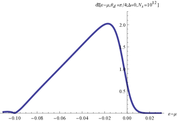
Figure 1: The number of photoelectrons $d\mathbf{I}(\theta_{d},\phi_{d},\epsilon)$ for $\Delta=0$

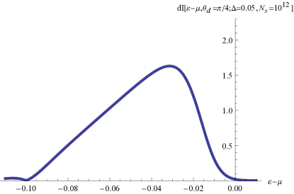
Figure 2: The number of photoelectrons $d\mathbf{I}(\theta_{d},\phi_{d},\epsilon)$ for $\Delta=0.05eV$

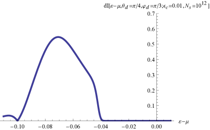
Figure 3: The number of photoelectrons $d\mathbf{I}(\theta_{d},\phi_{d},\epsilon)$ for $\epsilon_{c}=0.05eV$, $\phi_{d}=\frac{\pi}{3}$

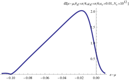
Figure 4: The number of photoelectrons $d\mathbf{I}(\theta_{d},\phi_{d},\epsilon)$ for $\epsilon_{c}=0.05eV$, $\phi_{d}=\frac{\pi}{6}$

Each time the angle $\phi_{d}=(2n+1)\frac{\pi}{6}$, $n=0,1,2,..$ the intensity is maximum and is minimum when the angles are $\phi_{d}=(2n+1)\frac{\pi}{3}$.

IV- The spin density in the $y$ direction measured by the detector at the polar angle $\phi_{d}$,$\theta_{d}$ as a function of the incoming photons $\vec{e}_{s=1,2}(\theta,\phi)$

The spin polarization of the $TI$ surface is given in terms of the spinor states $U_{\alpha}(\vec{K})$ with $\alpha=\uparrow,\downarrow$. The momentum parallel to the surface is conserved, the chiral angle satisfies $\cos[\phi_{d}]=\cos[\chi]$. The spin polarization $\langle\sigma^{y}\rangle\equiv S^{y}=\cos[\phi_{d}](\sin[\beta[\hat{\epsilon},\Delta,\epsilon_{c}])^{\frac{3}{2}}\Theta[\hat{\epsilon}]$ is recorded by the detector as $\mathbf{\hat{P}}^{y}_{s}(\theta,\phi,\phi_{d},\hat{\epsilon})$. $\sin[\beta[\hat{\epsilon},\Delta,\epsilon_{c}]$ represent the effect of the Zeeman gap $\Delta$ or ,$\epsilon_{c}$ for warping. The function $(\sin[\beta[\hat{\epsilon},\Delta,\epsilon_{c}])^{\frac{3}{2}}$ is given for the gap $\Delta$ and warpping $\epsilon_{c}$,

$$P_{pol.-supr.}[\hat{\epsilon}+\mu,\Delta]\equiv(\sin[\beta[\hat{\epsilon},\Delta)])^{\frac{3}{2}}=\Big{(}\frac{(\hat{\epsilon}+\mu)^{2}}{(\hat{\epsilon}+\mu)^{2}+\Delta^{2}}\Big{)}^{\frac{3}{2}}$$

$$P_{pol.-supr.}[\hat{\epsilon}+\mu,\epsilon_{c}]\equiv(\sin[\beta[\hat{\epsilon},\epsilon_{c})])^{\frac{3}{2}}=\Big{(}\frac{1}{1+(\frac{\hat{\epsilon}+\mu}{\epsilon_{c}})^{4}\cos^{2}(3\phi_{d})}\Big{)}^{\frac{3}{2}}$$

Using the definition given in Eqs.$(4-6)$ we obtain the relation between $S^{y}$ and $\mathbf{\hat{P}}^{y}_{s}(\theta,\phi,\phi_{d}\hat{\epsilon},\Delta=\epsilon_{c}=0)$:

$$\mathbf{\hat{P}}^{y}_{s}(\theta,\phi,\phi_{d},\hat{\epsilon},\Delta=\epsilon_{c}=0)=S^{y}\sum_{i,j=1,2}\mathbf{M_{s}(i,j|\theta,\phi)}W_{i}(\phi_{d},\hat{\epsilon})W_{j}(\phi_{d},\hat{\epsilon})W_{i}(\phi_{d},\hat{\epsilon})$$

The spin density for the linear for the $\mathbf{p}$ polarization polarization corresponds to $\vec{e}_{s=1}(\phi=0,\theta)$,and the $\mathbf{s}$ polarization is corresponds to $\vec{e}_{s=2}(\phi=0)$. We find:

$$\mathbf{\hat{P}}^{y}_{s=1}(\theta,\phi=0,\phi_{d},\Delta=\epsilon_{c}=0)=S^{y}\cos^{2}[\theta]\cos^{2}[\phi_{d}]$$

$$\mathbf{\hat{P}}^{y}_{s=2}(\phi=0,\phi_{d},\Delta=\epsilon_{c}=0)=S^{y}\sin^{2}[\phi_{d}]$$

The detection of the spin polarization is affected by the photon polarization. We have the relation:

$$\mathbf{\hat{P}}^{y}_{s=2}(\frac{\pi}{2}-\phi_{d},)\cos^{2}[\theta]=\mathbf{\hat{P}}^{y}_{s=1}(\theta,\phi_{d})$$ (18)

In figure $5$ shows the polarizations for $\Delta=\epsilon_{c}=0$. $\mathbf{\hat{P}}^{y}_{s=1}(\theta_{d}=\frac{\pi}{4},\phi_{d})$ represents the $\mathbf{p}$ polarization and $\mathbf{\hat{P}}^{y}_{s=2}(\theta_{d}=\frac{\pi}{4},\phi_{d})$ is the result for the $\mathbf{p}$ polarization.

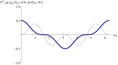
Figure 5: $\mathbf{\hat{P}}^{y}_{s}(\theta_{d}=\frac{\pi}{4},\phi_{d})$ for $\Delta=\epsilon_{c}=0$. The thick line represents the $\mathbf{p}$ polarization $\mathbf{P}^{y}_{s=1}$ and the thin line represents the $\mathbf{s}$ polarization $\mathbf{P}^{y}_{s=2}$

For a finite gap $\Delta$ the polarization is suppressed by the energy factor $(\sin[\beta[\hat{\epsilon},\Delta)])^{\frac{3}{2}}$.

For warping figure $6$ shows the warping caused by the angle $\phi_{d}$, $(\sin[\beta[\hat{\epsilon},\epsilon_{c})])^{\frac{3}{2}}$.

Figure 6: $\mathbf{\hat{P}}^{y}_{s=1}(\theta_{d}=\frac{\pi}{4},\phi_{d})$ for $\epsilon_{c}=0.05$ at the fixed energy.

V-Conclusions

To conclude, a model for computing the photoelectrons intensity and polarization from the surface of a topological insulator based on Green’s functions has been introduced. We show that the polarization of photoelectrons depends on the laser light polarization in qualitative agreement with experimental results Nature . The photoelectrons polarization is modified by the incoming photon polarization. This results hold also in the presence of a Zeeman gap or warping. For the Zeeman gap the polarization and intensity is suppressed closed to the Fermi energy. For warping the polarization and the intensity oscillates with the warping angle $\phi_{d}$ allowing to identify the spin texture.

The calculation is based on the tunneling amplitude of the surface electrons into the vacuum .This amplitude can be estimated from the inverted and vacuum $TI$ gap. We compute the number of the emitted photoelectrons. This number depends tunneling amplitude, chemical potential,incoming number of photons and weakly dependent on the location of the detector. Our calculation indicate that for $\tau=0.1$, $\mu=0.1eV$, $K_{F}L=10^{7}$ and $N_{s}=10^{12}$ we obtain that the maximum number of photoelectrons is approximately $2$.

The calculation ignores the bulk electrons, therefore the intensity computed can not be compared with the experimental results for energy $\epsilon-\mu<-\mu$ (the bottom of the surface states are at $\epsilon_{0}=\hbar v|\vec{K}|=0$ , in figures $1-4$ this corresponds to $\epsilon-\mu=-0.1eV$ )

References

(1) B.A. Volkov and O.A. Pankratov, JETP Lett. 61, 2015 (1988).
(3) C.L. Kane and E.J. Mele, Phys. Rev. Lett. 75, 146802 (2005).
(4) D. Schmeltzer, in Advances in Condensed Matter and Materials Research, Vol. 10, edited by Hans Geelvinck and Sjaak Reyst (Nova Science Hauppauge, New York, 2011), Chap. , pp. 379-403.
(5) Chris Jozwiak, Cheol-Hwan, Keneth Gothlieb, Choongyu Hwang, Dung-Hai Lee, Steven G. Louie, Jonathan D. Denlinger, Costel R. Rotundu, Robert Bitgeneau, Zahid Hussain, and Alessandra Lanzara, Nature Phys. 9, 293 (2013).
(6) Q.-K. Xue, Nature Phys. 9, 265 (2013).
(7) Oleg V. Yazyev, Joel Moore, and Steven G. Louie, Phys. Rev. Lett 105, 266806 (2010).
(8) Cheo-Hwan Park and Steven G. Louie, Phys. Rev. Lett. 109, 097601 (2012).
(9) Y.H. Wang, D. Hsieh, D. Pilon, L. Fu, D.R. Gardner, Y.S. Lee, and N. Gedik, Phys. Rev. Lett. 107, 207602 (2011).
(10) Z.-H. Zhu, C. N. Veenstra, S. Zhdanovich, M.P. Schneider, T. Okuda, K. Miyamoto, S.-Y. Zhu, and H. Namatame, Phys. Rev. Lett. 112, 076802 (2014).
(11) S Suga et al., J. Phys. Soc. Jpn. 83, 014705 (2014).
(12) Z. Xie et al., Nature Commun. 5, 3382 (2014).
(13) Lin Miao, Z.F. Wang, Wenmei Ming, Meng-Yu Yao, Meixiano Wang, Fang Yang, Y.R. Song, Fengfeng Zhu, Alexei V. Fedorov, Z. Sun, C.L. Gao, Canhua Liu, Qi-Kun Xue, Chao-Xing Liu, Feng Liu, Dong Qian, and Jin-Feng Jia, Proc. Nat. Acad. Sci. (USA) 10, 2758 (2013).
(14) J.W. McIver, D. Hsieh, P. Jarillo-Herrero, and N. Gedik, Nat. Nanotech. 7, 96 (2011).
(15) A. Junck, G. Refael, and F. von Oppen, Phys. Rev. B 88, 075144 (2013).
(16) Fan Zhang, C.L. Kane, and E.J. Mele, Phys. Rev. B 86, 081303(R) (2012).
(17) D. Schmeltzer and Avadh Saxena, Phys. Rev. B 88, 035140 (2013).
(18) Liang Fu, Phys. Rev. Lett 103, 266801 (2009).
(19) S. Doniach and E. H. Sondheimer “Green’s Functions for Solid State Physicists” (Imperial College Press, London, 1988).