Approximation Algorithms for Reducing the Spectral Radius To Control Epidemic Spread

Abstract

The largest eigenvalue of the adjacency matrix of a network (referred to as the spectral radius) is an important metric in its own right. Further, for several models of epidemic spread on networks (e.g., the ‘flu-like’ SIS model), it has been shown that an epidemic dies out quickly if the spectral radius of the graph is below a certain threshold that depends on the model parameters. This motivates a strategy to control epidemic spread by reducing the spectral radius of the underlying network.

In this paper, we develop a suite of provable approximation algorithms for reducing the spectral radius by removing the minimum cost set of edges (modeling quarantining) or nodes (modeling vaccinations), with different time and quality tradeoffs. Our main algorithm, GreedyWalk, is based on the idea of hitting closed walks of a given length, and gives an $O(\log^{2}{n})$-approximation, where $n$ denotes the number of nodes; it also performs much better in practice compared to all prior heuristics proposed for this problem. We further present a novel sparsification method to improve its running time.

In addition, we give a new primal-dual based algorithm with an even better approximation guarantee ($O(\log n)$), albeit with slower running time. We also give lower bounds on the worst-case performance of some of the popular heuristics. Finally we demonstrate the applicability of our algorithms and the properties of our solutions via extensive experiments on multiple synthetic and real networks.

1 Introduction

Given a contact network, which contacts should we remove to contain the spread of a virus? Equivalently, in a computer network, which connections should we cut to prevent the spread of malware? Designing effective and low cost interventions are fundamental challenges in public health and network security. Epidemics are commonly modeled by stochastic diffusion processes, such as the so-called ‘SIS’ (flu-like) and ‘SIR’ (mumps-like) models on networks (more in Section 2). An important result that highlights the impact of the network structure on the dynamics is that epidemics die out “quickly” if $\rho(G)\leq T$, where $\rho(G)$ is the spectral radius (or the largest eigenvalue) of graph $G$, and $T$ is a threshold that depends on the disease model [14, 39, 31]. This motivates the following strategy for controlling an epidemic: remove edges (quarantining) or nodes (vaccinating) to reduce the spectral radius below a threshold $T$—we refer to this as the spectral radius minimization (SRM) problem, with variants depending on whether edges are removed (the SRME problem) or whether nodes are removed (the SRMN problem). Van Mieghem et al. [28] and Tong et al. [37] prove that this problem is NP-complete. They also study two heuristics for it, one based on the components of the first eigenvector (EigenScore) and another based on degrees (ProductDegree). However, no rigorous approximations were known for the SRME or the SRMN problems.

Our main contributions.

1. Lower bounds on the worst-case performance of heuristics: We show that the ProductDegree, EigenScore and Pagerank heuristics (defined formally in Section 2) can perform quite poorly in general. We demonstrate graph instances where these heuristics give solutions of cost $\Omega(\frac{n}{T^{2}})$ times the optimal, where $n$ is the number of nodes in the graph.

2. Provable approximation algorithms: We present two bicriteria approximation algorithms for the SRME and SRMN problems, with varying approximation quality and running time tradeoffs. Our first algorithm, GreedyWalk, is based on hitting closed walks in $G$. We show this algorithm has an approximation bound of $O(\log{n}\log{\Delta})$ times optimal for the cost of edges removed, while ensuring that the spectral radius becomes at most $(1+\epsilon)$ times the threshold, for $\epsilon$ arbitrarily small (here $\Delta$ denotes the maximum node degree in the graph). We also design a variant, GreedyWalkSparse, that performs careful sparsification of the graph, leading to similar asymptotic guarantees, but better running time, especially when the threshold $T$ is small. We then develop algorithm PrimalDual, which improves this approximation bound to an $O(\log{n})$ using a more sophisticated primal-dual approach, at the expense of a slightly higher (but polynomial) running time.

3. Extensions: We consider two natural extensions of the SRME problem: (i) non-uniform transmission rates on edges and (ii) node version SRMN. We show that our methods extend to these variations too.

4. Empirical analysis: We conduct an extensive experimental evaluation of GreedyWalk, a simplified version of PrimalDual and different heuristics that have been proposed for epidemic containment on a diverse collection of synthetic and real networks. These heuristics involve picking edges $e=(i,j)$ in non-increasing order of some kind of score; the specific heuristics we compare include: (i) ProductDegree, (ii) EigenScore, (iii) LinePagerank, and (iv) Hybrid, which picks the edge based on either the eigenscore or the product-degree ordering, depending on the maximum decrease in eigenvalue. We find that GreedyWalk performs better than all the heuristics in all the networks we study. We analyze GreedyWalk for walks of length $k=\Theta(\log{n})$; in practice, we found that the performance degrades significantly as $k$ is reduced.

Organization. The background and notation are defined in Section 2. Sections 3, 4 and 5 cover GreedyWalk, GreedyWalkSparse and PrimalDual algorithms, respectively, for the SMRE problem; the SRMN problem is discussed in section 6. Some of the algorithmic details and proofs are omitted for brevity and are available in [35]. Lower bounds for some heuristics and the experimental results are discussed in Sections 7 and 8, respectively. We discuss the related work in Section 9 and conclude in Section 10.

2 Preliminaries

Table 1: Notations

$G=(V,E)$	Graph representing a contact network
$n=|V|$	Total number of nodes in $G$
$d(v,G)$	Degree of node $v$ in $G$
$\Delta(G)$	Maximum node degree in $G$
$A=A^{G}$	Adjacency matrix of $G$
$G[E^{\prime}]$	Subgraph of $G$ induced on $E^{\prime}\subseteq E$
$\lambda_{i}(G)$	$i$th largest Eigenvalue of $A^{G}$
$\rho(G)=\rho(A)$	$\lambda_{1}(G)$, spectral radius of $G$
$c(\cdot)$	Cost of a vertex or edge of $G$
$\beta$	Infection rate
$\delta$	Recovery rate
$T$	Epidemic Threshold, $T=\frac{\delta}{\beta}$
$\tau$	Time to epidemic extinction
$\mathcal{W}_{k}(G)$	Set of closed walks of length $k$ in $G$
$W_{k}(G)$	$W_{k}(G)=|\mathcal{W}_{k}(G)|$
$\operatorname*{nodes}(w)$	number of distinct nodes in walk $w$
$\operatorname*{walks}(x,G,k)$	Number of closed $k$-walks in $G$ containing edge (or vertex) $x$
$E_{\mathrm{OPT}}(T)$	Optimal solution to SRME$(G,c(\cdot),T)$

We consider undirected graphs $G=(V,E)$, and interventions to control the spread of epidemics— vaccination (modeled by removal of nodes) and quarantining (modeled by removal of edges). There can be different costs for the removal of nodes and edges (denoted by $c(v)$ and $c(e)$, respectively), e.g., depending on their demographics, as estimated by [26]. For a set $E^{\prime}\subset E$, $c(E^{\prime})=\sum_{e\in E^{\prime}}c(e)$ denotes the total cost of the set $E^{\prime}$ (similarly for node subsets).

There are a number of models for epidemic spread; we focus on the fundamental SIS (Susceptible-Infectious-Susceptible) model, which is defined in the following manner. Nodes are in susceptible (S) or infectious (I) state. Each infected node $u$ (in state I) causes each susceptible neighbor $v$ (in state S) to become infected at rate $\beta_{uv}$. Further, each infected node $u$ switches to the susceptible state at rate $\delta$. In this paper, we assume a uniform rate $\beta_{uv}=\beta$ for all $(u,v)\in E$; in this case, we define a threshold $T=\delta/\beta$, which characterizes the time to extinction. Let $A=A^{G}$ denote the adjacency matrix of $G$, and let $n=|V|$. Let $\lambda_{i}(G)$ denote the $i$th largest eigenvalue of $A$, and let $\rho(A)=\lambda_{1}(A)$ denote the spectral radius of $A$. Since $G$ is undirected, it follows that all eigenvalues are real, and $\rho(A)>0$ (see, e.g., Chapter 3 of [27]). Ganesh et al. [14] showed that the epidemic dies out in time $O(\frac{\log{n}}{1-\rho(A)/T})$, if $\rho(A)<T$ in the SIS model, with high probability; this threshold was also observed by [39]. Prakash et al. [31] show this condition holds for a broad class of other epidemic models, including the SIR model (which contains the ‘Recovered’ state). Now we formally define the SRM problem.

Definition 2.1

Spectral Radius Minimization problems (SRME and SRMN): Given an undirected graph $G=(V,E)$, with cost $c(e)$ for each edge $e$, and a threshold $T$, the goal of the SRME$(G,c(\cdot),T)$ problem is to find the cheapest subset $E^{\prime}\subseteq E$ such that $\lambda_{1}(G[E\setminus E^{\prime}])<T$. We refer to the node version of this problem as SRMN$(G,c(\cdot),T)$.

We discuss some notation that will be used in the rest of the paper. $E_{\mathrm{OPT}}(T)$ denotes an optimal solution to the SRME$(G,c(\cdot),T)$ problem. Let $\mathcal{W}_{k}(G)$ denote the set of closed walks of length $k$ in $G$; let $W_{k}(G)=|\mathcal{W}_{k}(G)|$. For a walk $w$, let $\operatorname*{nodes}(w)$ denote the number of distinct nodes in $w$. A standard result (see, e.g., Chapter 3 of [27]) is the following:

(2.1) $$\sum_{w\in\mathcal{W}_{k}(G)}\operatorname*{nodes}(w)=\sum_{i}A^{k}_{ii}=\sum_{i=1}^{n}\lambda_{i}(G)^{k}.$$

The number of walks in $\mathcal{W}_{k}(G)$ containing a node $i$ is $A^{k}_{ii}$. For a graph $G$, let $\operatorname*{walks}(e,G,k)$ denote the number of closed $k$-walks in $G$ containing $e=(i,j)$. Then, $\operatorname*{walks}(e,G,k)=A^{k-1}_{ij}$. We say that an edge set $E^{\prime}$ hits a walk $w$ if $w$ contains an edge from $E^{\prime}$. Similarly, for a node $v$, let $\operatorname*{walks}(v,G,k)$ denote the number of closed $k$-walks in $G$ containing $v$. Then, $\operatorname*{walks}(i,G,k)=A^{k}_{ii}$. Table 1 summarizes the frequently used notations.

3 GreedyWalk: $O(\log{n}\log\Delta)$-approximation

Main idea. Our starting point is the connection between the number of closed walks in a graph and the sum of powers of the eigenvalues in (2.1). We try to reduce the spectral radius by reducing the number of closed walks of length $k$ in the graph, by removing edges (see Algorithm 1). This, in turn, can be viewed as a partial covering problem. Our basic idea extends to other versions, as discussed later in Section 6.

Algorithm 1 GreedyWalk (high level description)

0:  $G$, $T$, $c(\cdot)$, $k$ even

0:  Edge set $E^{\prime}$

1:  Initialize $E^{\prime}\leftarrow\phi$

2:  while $W_{k}(G[E\setminus E^{\prime}])\geq nT^{k}$ do

3:     $r\leftarrow W_{k}(G[E\setminus E^{\prime}])-nT^{k}$

4:     Pick $e\in E\setminus E^{\prime}$ that maximizes $\frac{\min\{r,\operatorname*{walks}(e,G[E\setminus E^{\prime}],k)\}}{c(e)}$

5:     $E^{\prime}\leftarrow E^{\prime}\cup\{e\}$

6:  end while

The Lemma below proves the approximation bound for any solution (say $E^{\prime}$) from GreedyWalk. Let $G^{\prime}=G[E\setminus E^{\prime}]$ denote the graph resulting after the removal of edges in $E^{\prime}$. Our proof involves three steps: (1) Proving the bound on $\lambda_{1}(G^{\prime})$; (2) Relating $c(E^{\prime})$ to the cost of the optimum solution to the partial covering problem which ensures that the number of walks in the residual graph is at most $nT^{k}$; (3) Showing that the optimum solution to the SRME problem also ensures that at most $nT^{k}$ remain in the residual graph.

Lemma 3.1

Let $E^{\prime}$ denote the set of edges found by Algorithm GreedyWalk. Given any constant $\epsilon>0$, let $k$ be an even integer larger than $\frac{\log{n}}{\log(1+\epsilon/3)}$. Then, we have $\lambda_{1}(G[E\setminus E^{\prime}])\leq(1+\epsilon)T$, and $c(E^{\prime})=O(c(E_{\mathrm{OPT}}(T))\log n\log\Delta)$.

• We follow the proof scheme mentioned above. By the stopping condition of the algorithm, we have $W_{k}(G^{\prime})\leqslant nT^{k}$. From (2.1), we have $\sum_{i=1}^{n}\lambda_{i}(G^{\prime})^{k}=\sum_{i}A_{ii}^{k}=\sum_{w\in\mathcal{W}(G^{\prime})}\operatorname*{nodes}(w)\leq kW_{k}(G^{\prime})$, which implies $\sum_{i=1}^{n}\lambda_{i}(G^{\prime})^{k}\leqslant nkT^{k}$. Further, since $k$ is even (by assumption), $\lambda_{i}(G^{\prime})\geq 0$, so that $\lambda_{1}(G^{\prime})^{k}\leq\sum_{i=1}^{n}\lambda_{i}(G^{\prime})^{k}\leq nkT^{k}$. This implies $\lambda_{1}(G^{\prime})\leqslant e^{(\log n+\log{k})/k}T$. Since $k=\log{n}/\log{(1+\epsilon/3)}$, we have $(\log n+\log{k})/k\leq 2\log{(1+\epsilon/3)}$, so that $\lambda_{1}(G^{\prime})\leq(1+\epsilon/3)^{2}T\leq(1+\epsilon)T$.

  Next, we derive a bound for $c(E^{\prime})$. Observe that the algorithm can be viewed as solving a partial cover problem, in which (i) the set $H$ of elements corresponds to walks in $\mathcal{W}_{k}(G)$, and (ii) there is a set corresponding to each edge $e\in E$ consisting of all the walks in $\mathcal{W}_{k}(G)$ that contain $e$. Following the analysis of the greedy algorithm for partial cover [36], we have $c(E^{\prime})=O(c(E_{\text{HITOPT}})\log|H|)$, where $E_{\text{HITOPT}}$ denotes the optimum solution for this covering instance. Since $\Delta$ denotes the maximum node degree, we have $H=W_{k}(G)\leqslant n{\Delta}^{k}$. We show below that $c(E_{\text{HITOPT}})\leq c(E_{\mathrm{OPT}}(T))$; it follows that $c(E^{\prime})=O(c(E_{\mathrm{OPT}}(T))\log n\log\Delta)$.

  Finally, we prove that $c(E_{\text{HITOPT}})\leq c(E_{\mathrm{OPT}}(T))$. By definition of $E_{\mathrm{OPT}}(T)$, we have $\lambda_{1}(G[E-E_{\mathrm{OPT}}(T)])\leq T$. Let $G^{\prime\prime}=G[E-E_{\mathrm{OPT}}(T)]$. Then, we have

  $$W_{k}(G^{\prime\prime})\leq\sum_{i=1}^{n}\lambda_{i}(G^{\prime\prime})^{k}<n\lambda_{1}(G^{\prime\prime})^{k}\leq nT^{k}.$$

  This implies $E_{\mathrm{OPT}}(T)$ hits at least $W_{k}(G)-nT^{k}$ walks, so that $c(E_{\text{HITOPT}})\leq c(E_{\mathrm{OPT}}(T))$.

Effect of the walk length $k$. We set the walk length $k=a\log{n}$ for some constant $a$ in Algorithm GreedyWalk; understanding the effect of $k$ is a natural question. From the proof of Lemma 3.1, it follows that $\lambda_{1}(G[E\setminus E^{\prime}])$ can be bounded by $(nk)^{1/k}T$ for any choice of $k$, as long as it is even. This bound becomes worse as $k$ becomes smaller, e.g., it is $O(\sqrt{n})$ for $k=2$. This is borne out in the experiments in Section 8.

In order to complete the description of GreedyWalk (Algorithm 1 ), we need to design an efficient method to determine the edge which maximizes the quantity in line 4. We discuss two methods below.

3.1 Matrix multiplication approach for implementing GreedyWalk.

Note that $\operatorname*{walks}(e,G,k)=A^{k-1}_{e}$. We use matrix multiplication to compute $A^{k-1}$ once for each iteration of the while loop in line 2 of Algorithm 1 . In line 4, we iterate over all edges, in order to compute the edge $e$ that maximizes the given ratio. For $k=O(\log n)$, $A^{k-1}$ can be computed in time $O(n^{\omega}\log\log{n})$, where $\omega<2.37$ is the exponent for the running time of the best matrix multiplication algorithm [40]. Therefore, each iteration involves $O(n^{\omega}\log\log{n}+m)=O(n^{\omega}\log\log{n})$ time. This gives a total running time of $O(n^{\omega}\log\log{n}|E_{OPT}|\log^{2}n)$, since only $O(|E_{OPT}|\log^{2}n)$ edges are removed. One drawback with this approach is the high (super-linear) space complexity, even with the best matrix multiplication methods, in general.

3.2 Dynamic programming approach for implementing GreedyWalk.

When the graphs are very sparse ($\Theta(n)$ edges), we adapt a dynamic programming approach to compute $\operatorname*{walks}(e,G,k)$ for an edge $e$ and more efficiently select the edge that maximizes $\operatorname*{walks}(e,G[E\setminus E^{\prime}],k)/c(e)$ in line 4 of Algorithm 1 . Although, potentially $\operatorname*{walks}(e,G,k)$ needs to be computed for each edge $e\in E\setminus E^{\prime}$, in practice it suffices to compute it for only a small subset of $E\setminus E^{\prime}$. We make use of the fact that $\operatorname*{walks}(e,G^{\prime},k)\leq\operatorname*{walks}(e,G,k)$ for any subgraph $G^{\prime}$. The approach is briefly as follows. Initially we compute $\operatorname*{walks}(e,G,k)$ for each $e\in E$ and arrange the edges in non-ascending order of their $\operatorname*{walks}(e,G,k)$ value, $e_{1},e_{2},...,e_{|E|}$. After the first edge ( i.e. $e_{1}$ in the first iteration) is removed, $\operatorname*{walks}(e,G^{\prime},k)$ is computed on the residual graph $G^{\prime}$ only for some consecutive edges in that order upto some $e_{i}$ such that $\operatorname*{walks}(e_{i},G^{\prime},k)>\operatorname*{walks}(e_{i+1},G,k)$. Edges $e_{2},...,e_{i}$ are reordered based on the recomputed walk numbers, $\operatorname*{walks}(e_{i},G^{\prime},k)$ and then the same steps are repeated. The approach takes $O(n)$ space and $O(n^{2}k)$ time assuming the number of edges is $\Theta(n)$ in real world large networks. The detailed algorithm and the analysis is given in the appendix A.1.

4 Using sparsification for faster running time: Algorithm GreedyWalkSparse

The efficiency of Algorithm GreedyWalk can be improved if the number of edges in the graph can be reduced. This can be achieved by two pruning steps - pruning edges such that in the residual graph (i) no node has degree more than $T^{2}$, and (ii) there is no $T$-core; the $T$-core of a graph denotes the maximal subgraph of $G$ with minimum degree $T$ (see, e.g., [3]). We will refer to these steps as MaxDegreeReduction and DensityReduction respectively. This leads to sparser graphs, without affecting the asymptotic approximation guarantees. The algorithm involves two prunning steps: MaxDegreeReduction and DensityReduction; the procedure is described in Algorithm GreedyWalkSparse.

Algorithm 2 Algorithm GreedyWalkSparse

0:  $G,T,c(\cdot)$

0:  Edge set $E^{\prime}$

1:  Initialize $G_{r}=G$.

2:  //Pruning step 1: MaxDegreeReduction

3:  Let $V_{T^{2}}=\{v:\mathrm{d}(v,G)\geqslant T^{2}\}$.

4:  for $v\in V_{T^{2}}$ do

5:     if $\mathrm{d}(v,G_{r})\geq T^{2}$ then

6:        Let $e_{v,1},\ldots,e_{v,\mathrm{d}(v,G_{r})}$ be the edges incident on $v$ ordered so that $c(e_{v,1})\leq\ldots\leq c(e_{v,\mathrm{d}(v,G_{r})})$.

7:        Let $E_{v}=\{e_{v,1},\dots,e_{v,\mathrm{d}(v,G_{r})-T^{2}+1}\}$.

8:        $E_{1}\leftarrow E_{1}\cup E_{v}$ and $E(G_{r})\leftarrow E(G_{r})\setminus E_{v}$.

9:     end if

10:  end for

11:  //pruning step 2: DensityReduction

12:  Let $C_{T}$ denote the $T$-core of $G_{r}$.

13:  Order the edges $e_{1},\ldots,e_{|E(C_{T})|}$ in non-decreasing order of cost.

14:  $E_{2}\leftarrow\{e_{i}\mid i\leq|E(C_{T})|-T|V(C_{T})|/2+1\}$

15:  //GreedyWalk on Pruned Graph:

16:  $E(G_{r})\leftarrow E(G_{r})-E_{1}-E_{2}$

17:  $E_{3}=\textsc{GreedyWalk}(G_{r},T,c(\cdot))$

18:  $E^{\prime}\leftarrow E_{1}\cup E_{2}\cup E_{3}$

Lemma 4.1

Let $E_{1}$ and $E_{2}$ denote the set of edges removed in the pruning steps MaxDegreeReduction and DensityReduction, respectively. Then, $c(E_{1})$ and $c(E_{2})$ are both at most $2c(E_{\mathrm{OPT}}(T))$.

• Since $\sqrt{\Delta(G^{\prime})}\leqslant\lambda_{1}(G^{\prime})$ [27], which implies $\Delta(G[E-E_{\mathrm{OPT}}(T)])\leq T^{2}$. Therefore, $c(\{e\in N(v)\cap E_{\mathrm{OPT}}(T)\})\geq\sum_{j=1}^{\mathrm{d}(v,G)-T^{2}+1}c(e_{v,j})$, where the sum is the minimum cost of edges that can be removed to ensure that the degree of $v$ becomes at most $T^{2}$. Therefore,

  $$c(E_{1}) =\sum_{v\in V_{T^{2}}}\sum_{j=1}^{\mathrm{d}(v,G)-T^{2}+1}c(e_{v,j})$$

  $$\leq\sum_{v\in V_{T^{2}}}c(\{e\in N(v)\cap E_{\mathrm{OPT}}(T)\})$$

  $$\leq c(E_{\mathrm{OPT}}(T))$$

  Recall that the second pruning step is applied on $G_{r}$. For bounding $c(E_{2})$, we use another lower bound for $\lambda_{1}$: for any induced subgraph $H$ of $G_{r}$, $\sum_{v\in V(H)}\frac{d(v,H)}{|V(H)|}\leq\lambda_{1}(G_{r})$. Therefore, the existence of a $T$-core $C_{T}$ implies that $\lambda_{1}(G_{r})\geq T$. Since the average degree of $C_{T}$ in the residual graph is at least $T$, it implies that at least $|E(C_{T})|-T|V(C_{T})|/2+1$ edges must be removed from $C_{T}$. Therefore,

  $$c(E_{2})=\sum_{j=1}^{|E(C_{T})|-T|V(C_{T})|/2+1}c(e_{j})\leq c(E_{\mathrm{OPT}}(T)\cap E(C_{T}))\,,$$

  where, the $e_{j}$ correspond to the first $|E(C_{T})|-T|V(C_{T})|/2+1$ edges of least cost. Hence proved.

By Lemma 4.1, it follows that the approximation bounds of Lemma 3.1 still hold. However, the pruning steps reduce the number of edges, thereby speeding the implementation of GreedyWalk. We discuss the empirical performance of pruning in Section 8. We show below that pruning also improves the approximation factor marginally from $O(\log n\log\Delta)$ to $O(\log n\log T)$ which could be significant when $n$ is large and $T\ll\Delta$.

Lemma 4.2

Let $E^{\prime}$ denote the set of edges found by Algorithm GreedyWalkSparse. Given any constant $\epsilon>0$, let $k$ be an even integer larger than $\frac{\log{n}}{\log(1+\epsilon/3)}$. Then, we have $\lambda_{1}(G[E\setminus E^{\prime}])\leq(1+\epsilon)T$, and $c(E^{\prime})=O(c(E_{\mathrm{OPT}}(T))\log n\log T)$.

• From Lemma 4.1, the number of edges removed is at most $2c(E_{\mathrm{OPT}})$. The residual graph $G_{r}$ has maximum degree less than $T^{2}$. Therefore, applying Lemma 3.1 on $G_{r}$, it follows that the number of edges removed is $O(c(E_{\mathrm{OPT}}(T))\log n\log T)$. Hence, the total number of edges removed by GreedyWalkSparse is at most $2c(E_{\mathrm{OPT}}(T))+O(c(E_{\mathrm{OPT}}(T))\log n\log T)=O(c(E_{\mathrm{OPT}}(T))\log n\log T)$.

5 PrimalDual: $O(\log{n})$-approximation

Main idea: The approach of [13] gives an $f$-approximation for the partial covering problem, where $f$ denotes the maximum number of sets that contain any element in the set system. As in the proof of Lemma 3.1, in our reduction from the SRME problem to partial covering, elements correspond to all the closed walks of length $k=O(\log{n})$, while sets correspond to edges; for an edge $e$, the corresponding set $S_{e}$ consists of all the walks $w$ that are hit by $e$. In this reduction, each walk $w$ lies in $k$ sets; therefore, $f=O(\log{n})$ for this set system. Therefore, the approach of [13] could improve the approximation factor. Unfortunately, our set system has size $n^{O(\log{n})}$, so that the algorithm of [13] cannot be used directly to get a polynomial time algorithm.

Algorithm 3 PrimalDual$(\mathcal{T}^{\prime},\mathcal{S}^{\prime},c^{\prime},\sigma^{\prime})$

0:  Edge set $E^{\prime\prime}$

1:  Initialize $z_{e}=0$ for all $S_{e}\in\mathcal{S}^{\prime}$, $C\leftarrow\phi$.

2:  //$u(w)=0$ for all walks $w$ in $G^{\prime}$.

3:  while $C$ is not $\sigma^{\prime}$-feasible do

4:     $x=\min_{e\in E\setminus E^{\prime\prime}}\{\frac{c(e)-z_{e}}{\operatorname*{walks}(e,G^{\prime},k)}\}$; let $e$ be an edge for which the minimum is reached.

5:     $C\leftarrow C\cup\{S_{e}\}$

6:     For each $e^{\prime}\in E\setminus E^{\prime\prime}$: $z_{e^{\prime}}=z_{e^{\prime}}+x\cdot\operatorname*{walks}(e^{\prime},G^{\prime},k)$

7:        //$u(w)=u(w)+x$ for all walks $w$ in $G^{\prime}$ that pass through $e^{\prime}$

8:     $E^{\prime}\leftarrow E^{\prime\prime}\cup\{e\}$

9:  end while

The algorithm of Gandhi et al. [13] uses a primal-dual approach, which maintains dual variables $u(w)$ for each element (i.e., walk); these are increased gradually, and a set (i.e., an edge) is picked if the sum of duals corresponding to the elements in the set equals its cost. We now discuss how to adapt this algorithm to run in polynomial time, and only focus on polynomial time implementation of the PrimalDual subroutine of [13] in detail here. However, we also present the set cover algorithm HitWalks for completeness. This algorithm iterates over all edges and invokes PrimalDual in each iteration to obtain a candidate set of edges to remove and finally chooses the set with minimum cost. $\mathcal{T}^{\prime}$, $\mathcal{S}^{\prime}$, $c^{\prime}$ and $\sigma^{\prime}$ denote the set of elements (walks) to be covered, the sets (corresponding to edges that can be chosen), the costs corresponding to the sets/edges and the number of elements (walks) that need to be covered, respectively. A subset $C\subseteq\mathcal{S}^{\prime}$ is $\sigma^{\prime}$-feasible if $|\cup_{S_{e}\in C}S_{e}|\geq\sigma^{\prime}$. Let $u(w)$ denote the dual variables corresponding to the walks $w$; these are not maintained in the algorithm explicitly, but assigned in the comments, for use in the analysis.

Algorithm 4 HitWalks$(\mathcal{T},\mathcal{S},c,\sigma)$

0:  Set of all $k$-closed walks $\mathcal{T}$, walks corresponding to edges $\mathcal{S}$, edge cost set $c$, number of walks to hit $\sigma$

0:  Edge set $E^{\prime}$

1:  Sort the edges of $G$ in increasing order of their costs.

2:  Initialize $\forall j$, $c^{\prime}(e_{j})\leftarrow\infty$

3:  for $j\leftarrow 1$ to $m$ do

4:     $c^{\prime}(e_{j})\leftarrow c(e_{j})$ and compute $\operatorname*{walks}(e_{j},G,k)$

5:      $cs_{j}\leftarrow\infty$. //cost of edge set in this iteration

6:     if $|S_{1}\cup S_{2}\cup\cdots S_{j}|\geqslant\sigma$ then

7:        $E^{\prime}_{j}~{}=~{}\{e_{j}\}~{}\cup~{}\textsc{PrimalDual}\big{(}\mathcal{T}~{}\setminus~{}S_{j},~{}\mathcal{S}~{}\setminus~{}S_{j},c^{\prime},\sigma-\operatorname*{walks}(e_{j},G,k)\big{)}$

8:        $cs_{j}=c(E^{\prime}_{j})$

9:     end if

10:     $i=\min_{j}cs_{j}$

11:     $E^{\prime}=E^{\prime}_{i}$

12:  end for

This algorithm does not explicitly update the dual variables, but the edges are picked in the same sequence as in [13].

Lemma 5.1

Given any constant $\epsilon>0$, let $k$ be an even integer larger than $\frac{\log{n}}{\log(1+\epsilon/3)}$. The dual variables $u(w)$ in algorithm PrimalDual are maintained and updated as in [13], and the edge $e$ picked in each iteration is the same. We have $c(E^{\prime})=O(c(E_{OPT})\log{n})$ and $\lambda_{1}(G[E\setminus E^{\prime}])\leq(1+\epsilon)T$.

• Instead of updating the dual variable $u(w)$ for each element (walk) $w$, as done in [13], the variable $z_{e}$ corresponding to each set (edge) $e$ is updated in algorithm PrimalDual at the end of each iteration. It is easy to see that, the following is an invariant at the end of each iteration, $z_{e}=\sum_{w\in S_{e}}u(w)$. Also note that, a set $e$ is picked into the cover in PrimalDual, whenever $z_{e}=c_{e}$.

  Therefore, increasing the $u(w)$’s has the same effect as increasing the $z_{e}$’s in terms of picking the sets into the cover and both the algorithm PrimalDual and the one in [13] chooses the same set in each iteration.

6 Node Version

Our discussion so far has focused on the SRME problem. We now consider extensions which capture two kinds of issues arising in practice.

1. Non-uniform transmission rates.

In general, the transmission rate $\beta$ is not constant for all the edges. The transmission rate $\beta_{ij}$ for edge $(i,j)$ depends on individual properties, especially the demographics of the end-points $i$ and $j$, such as age, e.g., [26]. Let $B=B(G)=(\beta_{ij})$ denote the matrix of the transmission rates. This gives us the SRME-nonuniform problem, which is defined as follows: Given an undirected graph $G=(V,E)$, with transmission rate $\beta_{ij}$ for each $(i,j)\in E$ and recovery rate $\delta$, find the smallest set $E^{\prime}\subseteq E$ such that $\rho(B(G[E-E^{\prime}]))\leq\delta$. We extend the spectral radius characterization of [14, 39, 31] to handle this setting, and show that GreedyWalk can also be adapted for solving SRME-nonuniform, with the same guarantees. The details of the algorithm, lemma and proofs are discussed in the appendix A.2.

2. The node removal version (SRMN problem).

We extend the GreedyWalk algorithm in a natural manner to work for SRMN, with the same approximation guarantees. For the details, please see the appendix A.3.

7 Popular heuristics and lower bounds

A number of heuristics have been developed for controlling the spread of epidemics– these are discussed below. All these heuristics involve ordering the edges based on some kind of score, and then selecting the top few edges based on this score. We describe the score function in each heuristic.

1. ProductDegree ([28]): The score for edge $e=(u,v)$ is defined as $\deg(u)\times\deg(v)$. Edges are removed in non-increasing order of this score.

2. EigenScore ([28, 37]): Let $\mathbf{x}$ be the eigenvector corresponding to the first eigenvalue of the graph. The score for edge $e=(u,v)$ is $|x(u)\times x(v)|$.

3. LinePagerank: This method uses the linegraph $L(G)=(E,F)$ of graph $G=(V,E)$, where $(e,e^{\prime})\in F$ if $e,e^{\prime}\in E$ have a common endpoint. We define the score of edge $e\in E$ as the pagerank of the corresponding node in $L(G)$.

As we find in Section 8.2, these heuristics work well for different kinds of networks. We design another heuristic, Hybrid, which picks the best of the EigenScore and ProductDegree methods. The edges are ordered in the following manner: (1) Let $\pi_{1},\ldots,\pi_{m}$ and $\mu_{1},\ldots,\mu_{m}$ be orderings of edges in the Eigenscore and ProductDegree algorithms, respectively. (2) Initialize $i=0$ and $j=0$, and (3) from the edges $\pi(i)$ and $\rho(j)$, remove the one which decreases the max eigenvalue of the residual graph more. Increment the corresponding index.

We have examined the worst case performance of these heuristics. Two of these, namely, EigenScore and ProductDegree, have been used specifically for reducing the spectral radius, e.g., [28, 37]. No formal analysis is known for any of these heuristics in the context of the SRME or SRMN problems; some of them seem to work pretty well on real world networks. We show that the worst case performance of these heuristics can be quite poor, in general.

Theorem 7.1

Given any sufficiently large positive integer $n$, there exists a threshold $T^{\prime}<a\sqrt{n}$, for some constant $a<1$ and a graph of size $n$ for which the number of edges removed by ProductDegree, EigenScore, Hybrid and LinePagerank is $\Omega\big{(}\frac{n}{T^{\prime 2}}\big{)}c(E_{\mathrm{OPT}})$.

The proof is presented in appendix A.4.

8 Experiments

8.1 Methods and Dataset

We evaluate the algorithms developed in the paper – GreedyWalk, GreedyWalkSparse and PrimalDual – and compare their performance with the heuristics from literature – EigenScore, ProductDegree, LinePagerank and Hybrid (described in Section 7), as a more sophisticated baseline. The networks which we considered in our empirical analysis are listed in Table 2 spanning infrastructure networks, social networks and random graphs.

Table 2: Networks and their sizes. The first two are synthetic random networks; others are taken from [2] and [1]

Network	nodes	edges	$\lambda_{1}$
Barabasi-Albert	$1000$	$1996$	$11.1$
Erdos-Renyi	$994$	$2526$	$6.38$
P2P (Gnutella05)	$8846$	$31839$	$23.55$
P2P (Gnutella06)	$8717$	$31525$	$22.38$
Collab. Net (HepTh)	$9877$	$25998$	$31.03$
Collab. Net (GrQc)	$5242$	$14496$	$45.62$
AS (Oregon 1)	$10670$	$22002$	$58.72$
AS (Oregon 2)	$10900$	$31180$	$70.74$
Brightkite Net	$58228$	$214078$	$101.49$
Youtube Network	$1134890$	$2987624$	$210.4$
Stanford Web graph	$281903$	$1992636$	$448.13$

8.2 Experimental results

Performance of our algorithms and comparison with other heuristics: We first compare the quality of solution from our algorithms with the EigenScore, ProductDegree, LinePagerank and Hybrid heuristics in Figure 1. We note that GreedyWalk is consistently better than all other heuristics, especially as the target threshold becomes smaller. Compared to the EigenScore, ProductDegree and LinePagerank heuristics, the spectral radius for the solution produced by GreedyWalk, as a function of the fraction of edges removed, is lower by at least 10-20%. Our improved baseline, the Hybrid heuristic, works better than the other heuristics, and comes somewhat close the GreedyWalk in many networks.

Though PrimalDual gives a significantly better approximation guarantee, compared to GreedyWalk, it has a much higher running time. Therefore, we only evaluate it for one iteration of Algorithm HitWalks. Figure 2 shows that PrimalDual is quite close to GreedyWalk after just one iteration; we expect running this algorithm fully would further improve the performance, but additional work is needed to improve the running time.

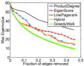
(a) AS Oregon-1

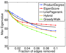
(b) AS Oregon-2

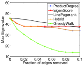
(c) Collaboration GrQc

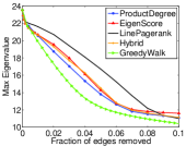
(d) P2P Gnutella-5

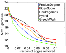
(e) P2P Gnutella-6

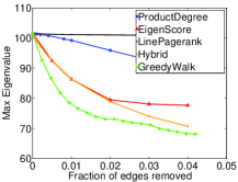
(f) Brightkite

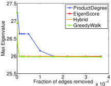
(g) Portland

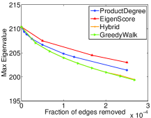
(h) Youtube

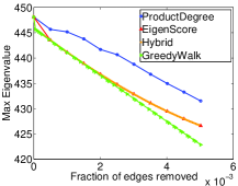
(i) Stanford Web

Figure 1: Comparison between the GreedyWalk, ProductDegree, Eigenscore, LinePagerank and Hybrid algorithms for different networks. Each plot shows the spectral radius (y-axis) as a function of the fraction of edges removed (x-axis). The LinePagerank heuristic has not been evaluated in 1g, 1h and 1i because of the scale of these networks.

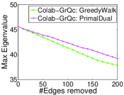
(a) Collaboration GrQc

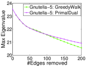
(b) P2P Gnutella-5

Figure 2: GreedyWalk vs PrimalDual. Each plot shows the spectral radius (y-axis) as a function of the number of edges removed (x-axis) using the two methods.

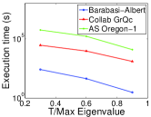
Figure 3: Total running time of GreedyWalk method (y-axis) as a function of $T/\rho(G)$ (x-axis), where $T$ is the threshold and $\rho(G)$ is the spectral radius of the initial graph, without any edges removed.

Running time and effect of sparsification:. Figure 3 shows the total running time of GreedyWalk for three networks. The time decreases with the increase of $T$, because the while loop in Algorithm GreedyWalk needs to be run for fewer iterations. The high running time motivates faster methods. We evaluate the performance of the GreedyWalkSparse algorithm. As shown in Figure 4, GreedyWalkSparse gives almost the same quality of approximation as GreedyWalk, but improves the running time by up to an order of magnitude, particularly when $T$ is small.

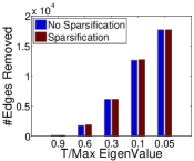
(a) #Edges removed

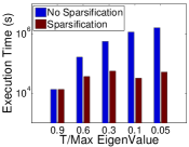
(b) Execution time

Figure 4: Impact of sparsification on GreedyWalk. The plots show for AS Oregon-1 network, (a) the number of edges removed and (b) the execution time on the y-axis, as a function of $T/\rho(G)$ (x-axis), where $T$ is the threshold and $\rho(G)$ is the spectral radius of the initial graph, without any edges removed.

Effect of varying walk lengths: As discussed in Section 3, the walk length parameter $k$ is critical for the performance of GreedyWalk. Figure 5 shows the approximation quality in the Oregon-2 and collaboration networks. We find that as $k$ becomes smaller, the approximation quality degrades significantly, and the best performance occurs at $k$ close to $2\log{n}$.

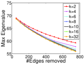
(a) AS Oregon-2

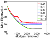
(b) Collaboration GrQc

Figure 5: Impact of walk length on GreedyWalk performance. Each plot shows the drop in spectral radius (y-axis) with number of edges removed (x-axis), for different values of $k$, ranging from $2$ to $2\log{n}$, for the corresponding networks.

Extensions: For the SRME-nonuniform problem, we compare the adaptation of GreedyWalk, as discussed in Section 6, with the Eigenscore heuristic run on the matrix $B$ of transmission rates. As shown in Figure 6b, we find that GreedyWalk performs much better. Next we consider the SRMN problem, and compare the GreedyWalk, as adapted in Section 6, with the node versions of the Degree and EigenScore heuristic [37]. As shown in Figure 6d, GreedyWalk performs consistently better. For results in other networks, see the full version [35].

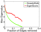
(a) SRME-nonuniform: Barabasi-Albert

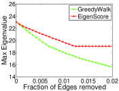
(b) SRME-nonuniform: Collaboration GrQc

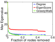
(c) SRMN: Oregon-1

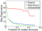
(d) SRMN: Collaboration GrQc

Figure 6: Computing solutions for SRME-nonuniform (6a,6b) and SRMN (6c,6d) problem on different networks with GreedyWalk algorithm and Degree and EigenScore heuristics as adapted in Section 6. The plots show the resultant spectral radius (y-axis) as fractions of edges/nodes are removed (x-axis) with different methods.

Demographic properties of removed nodes and edges: GreedyWalk can also help in getting non-network surrogates for picking nodes/edges. We analyzed the demographic properties of the nodes and edges removed by GreedyWalk on the Portland contact network [1]. By doing so, we can hope to use such demographic properties directly, for quicker implementation and/or when the entire network is not readily available. Figure 7 shows the age groups of the end points of the top $1500$ selected edges by GreedyWalk as a matrix. Age-groups are partitioned according to [26] and shown in table 3. As the figure shows, the edges among age-group #$11$ (ages $45-49$) and with age-groups #$8$ (age $30-34$) and #$17$ (age $75+$) are picked to a greater extent by GreedyWalk. We observe that the edges picked by GreedyWalk have substantially different properties compared to other heuristics . Figure 8 shows the age groups of the nodes removed by the GreedyWalk algorithm for the SRMN problem, along with the age group distribution of the entire population. Observe that more people are selected in age-group numbers 7 to 11 which correspond to ages 25-49.

Table 3: Age-groups [26]

Age-group	Age	Age-group	Age
1	0	10	40-44
2	1-4	11	45-49
3	5-9	12	50-54
4	10-14	13	55-59
5	15-19	14	60-64
6	20-24	15	65-69
7	25-29	16	70-74
8	30-34	17	75+
9	35-39

(a) Removed Edges

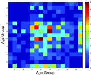
(b) ProductDegree

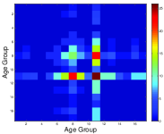
(c) ProductEigenscore

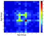
(d) Hybrid

Figure 7: Age-Group matrix of the top 1500 removed edges

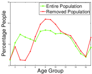
(a) Removed Nodes

Figure 8: Age-group of 1500 removed nodes with GreedyWalk from Portland contact graph.

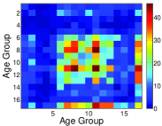
(a) Removed Edges

(b) Removed Nodes

Figure 9: (9a) Age-Group matrix of the top 1500 removed edges and (9b) Age-group of 1500 removed nodes with GreedyWalk from Portland contact graph.

Main observations:

1. GreedyWalk performs consistently better than existing heurisitics in removing nodes or edges in both static and variable transmission rate settings.

2. Sparsification helps in improving the speed of GreedyWalk without effecting the solution quality.

3. GreedyWalk performs best for walk-lengths of $k=2\log n$.

4. GreedyWalk can potentially help in picking more accurate non-network surrogates.

9 Related Work

Related work comes from multiple areas: epidemiology, immunization algorithms and other optimization algorithms. There is general research interest in studying dynamic processes on large graphs, (a) blogs and propagations [17, 22], (b) information cascades [15, 16] and (c) marketing and product penetration [34]. These dynamic processes are all closely related to virus propagation.

Epidemiology: A classical text on epidemic models and analysis is by May and Anderson [4]. Most work in epidemiology is focused on homogeneous models [6, 4]. Here we study network based models. Much work has gone into in finding epidemic thresholds (minimum virulence of a virus which results in an epidemic) for a variety of networks [29, 39, 14, 31].

Immunization: There has been much work on finding optimal strategies for vaccine allocation [7, 25, 11]. Cohen et al [12] studied the popular acquaintance immunization policy (pick a random person, and immunize one of its neighbors at random). Using game theory, Aspnes et al. [5] developed inoculation strategies for victims of viruses under random starting points. Kuhlman et al. [21] studied two formulations of the problem of blocking a contagion through edge removals under the model of discrete dynamical systems. As already mentioned Tong et al. [38, 37], Van Miegham et al. [28], Prakash et al. [30] and Chakrabarti et al. [9] proposed various node-based and edge-based immunization algorithms based on minimizing the largest eigenvalue of the graph. Other non-spectral approaches for immunization have been studied by Budak et al [8], He et al [18] and Khalil et al. [20].

Other Optimization Problems: Other diffusion based optimization problems include the influence maximization problem, which was introduced by Domingos and Richardson [33], and formulated by Kempe et. al. [19] as a combinatorial optimization problem. They proved it is NP-Hard and also gave a simple $1-1/e$ approximation based on the submodularity of expected spread of a set of starting seeds. Other such problems where we wish to select a subset of ‘important’ vertices on graphs, include ‘outbreak detection’ [24] and ‘finding most-likely culprits of epidemics’ [23, 32].

10 Conclusions

We study the problem of reducing the spectral radius of a graph to control the spread of epidemics by removing edges (the SRME problem) or nodes (the SRMN problem). We have developed a suite of algorithms for these problems, which give the first rigorous bounds for these problems. Our main algorithm GreedyWalk performs consistently better than all other heuristics for these problems, in all networks we studied. We also develop variants that improve the running time by sparsification, and improve the approximation guarantee using a primal dual approach. These algorithms exploit the connection between the graph spectrum and closed walks in the graph, and perform better than all other heuristics. Improving the running time of these algorithms is a direction for further research. We expect these techniques could potentially help in optimizing other objectives related to spectral properties, e.g., robustness [10], and in other problems related to the design of interventions to control the spread of epidemics.

Acknowledgments. This work has been partially supported by the following grants: DTRA Grant HDTRA1-11-1-0016, DTRA CNIMS Contract HDTRA1-11-D-0016-0010, NSF Career CNS 0845700, NSF ICES CCF-1216000, NSF NETSE Grant CNS-1011769, DOE DE-SC0003957, National Science Foundation Grant IIS-1353346 and Maryland Procurement Office contract H98230-14-C0127. Also supported by the Intelligence Advanced Research Projects Activity (IARPA) via Department of Interior National Business Center (DoI/NBC) contract number D12PC000337, the US Government is authorized to reproduce and distribute reprints for Governmental purposes notwithstanding any copyright annotation thereon.
Disclaimer: The views and conclusions contained herein are those of the authors and should not be interpreted as necessarily representing the official policies or endorsements, either expressed or implied, of IARPA, DoI/NBC, or the US Government.

A Appendix

A.1 GreedyWalk with Dynamic Programming Approach

Main idea: we adapt a dynamic programming approach in sparse graphs to avoid matrix multiplication, that leads to lower space complexity, thereby allowing us to scale to larger graphs. We then observe that the number of walks does not need to be recomputed each time an edge is deleted.

Let $H_{\overrightarrow{uv}}(G,x,l)$ denote the number of walks of length $l$ from node $u$ through edge $(u,v)$ as the first edge to node $x$ in $G$. It is easy to see that, $H_{\overrightarrow{uv}}(G,u,k)=\operatorname*{walks}(e,G,k)$. Algorithm ClosedWalkDP describes how to compute $H_{\overrightarrow{uv}}(G,u,l)=\operatorname*{walks}(e,G,k)$. In the algorithm, $N(x)$ denotes the neighbors of node $x$ in $G$.

Algorithm 5 $\textsc{ClosedWalkDP}(G,(u,v),k)$

0:  $G,(u,v),k\geq 2$

0:  Number of closed walks of length $k$ in $G$ containing $(u,v)$

1:  Let $H_{\overrightarrow{uv}}(G,v,1)=1$, $H_{\overrightarrow{uv}}(G,x,1)=0$, $\forall x\in V\setminus\{v\}$

2:  for $l=2$ to $k$ do

3:     $H_{\overrightarrow{uv}}(G,x,l)=\sum_{y\in N(x)}H_{\overrightarrow{uv}}(G,y,l-1)$, $\forall x\in V$

4:  end for

5:  return $H_{\overrightarrow{uv}}(G,u,k)$

Next, we describe in Algorithm GreedyEdgeChoice how the greedy edge choice in line 4 of Algorithm GreedyWalk is implemented efficiently. We make use of the fact that $\operatorname*{walks}(e,G^{\prime},k)\leq\operatorname*{walks}(e,G,k)$ for any $G^{\prime}\subset G$. In every iteration of Algorithm GreedyEdgeChoice, potentially, we need to update $f(\cdot)$ for all edges in $E\setminus E^{\prime}$. However, in practice, we observe that the number of such updates is very small compared to $|E\setminus E^{\prime}|$.

Algorithm 6 GreedyEdgeChoice

0:  $G,T,c(\cdot)$

0:  Edge set $E^{\prime}$

1:  Initialize $E^{\prime}\leftarrow\phi$ and $\forall e\in E$, let $f(e)=\operatorname*{walks}(e,G,k)$ //computed by ClosedWalkDP

2:  while $W_{k}(G[E\setminus E^{\prime}])\geq nT^{k}$ do

3:     Order edges of $E\setminus E^{\prime}$ in the decreasing order of $f(.)$ values. Let $e_{1}$ be the first edge.

4:     $E^{\prime}\leftarrow E^{\prime}\cup\{e_{1}\}$

5:     for $j=2,\ldots,|E\setminus E^{\prime}|$ do

6:        Update $f(e_{j})=\operatorname*{walks}(e_{j},G[E\setminus E^{\prime}],k)$.

7:        if $f(e_{j})\geq f(e_{j+1})$ then

8:           Exit from the for loop

9:        end if

10:     end for

11:  end while

Running time and space complexity: Let $n=|V|$, $m=|E|$. Note that, $\textsc{ClosedWalkDP}(G,e,k)$ takes $2mk$ time to compute $\operatorname*{walks}(e,G,k)$. Therefore, computing $\operatorname*{walks}(e,G,k)$ for all the edges takes $2m^{2}k=O(n^{2}k)$, assuming $m=\Theta(n)$ in real world networks. Since, for computing $H_{\overrightarrow{uv}}(G,x,l)$, $\forall x\in V$, $\textsc{ClosedWalkE}(k)$ needs to look only at $H_{uv}(G,y,l-1)$, $\forall y\in V$, therefore, the space complexity is $\Theta(n)$.

A.2 Non-uniform transmission rates

Let $B=(\beta_{ij})$ denote the matrix of the transmission rates. We assume the rates are symmetric, i.e., $\beta_{ij}=\beta_{ji}$. In this case, the sufficient condition for the epidemic to die out is slightly different, and is stated below.

Lemma A.1

Let $B$ be the matrix of transmission rates, and let $\delta$ be the recovery rate in the SIS model. If $\rho(B)<\delta$, the time to extinction, $\tau$ satisfies

$$\mathrm{Exp}[\tau]\leq\frac{\log{n}+1}{\delta-\rho(B)}$$

For the case of uniform costs, i.e., $c(e)=1$ for all edges $e$, this motivates the following problem:

Definition A.1

SRME-nonuniform problem Given an undirected graph $G=(V,E)$, with transmission rate $\beta_{ij}$ for each $(i,j)\in E$ and recovery rate $\delta$, find the smallest set $E^{\prime}\subseteq E$ such that $\rho(B(G[E-E^{\prime}]))\leq\delta$.

In this section, we use $E_{\mathrm{OPT}}$ to denote the optimum solution to SRME-nonuniform$(G,B,\delta)$. Our algorithm GreedyWalk-nonuniform adapts GreedyWalk to a weighted covering problem. We need to refine the definitions used earlier. For walk $w\in\mathcal{W}_{k}(G)$, let $f(w)=\prod_{e=(ij)\in E(w)}\beta_{ij}^{\operatorname*{count}(e,w)}$ denote its weight, where $\operatorname*{count}(e,w)$ is the number of occurrences of edge $e$ in walk $w$; for a set $W^{\prime}$ of walks, let $f(W^{\prime})=\sum_{w\in W^{\prime}}f(w)$ denote the total weight of $W^{\prime}$. In the algorithm, we will need to compute $f(W_{k}(G))$, which is done by modifying the recurrence used in Algorithm CountWalks$(G)$ to compute $W_{k}(G)$:

$$f(W_{k}(G))=B^{k}_{nn}+f(W_{k}(G[V-\{n\}]).$$

Let $f(e,G)=\sum_{w:e\in w}f(w)$ denote the total weight of walks containing edge $e$; $f(e,G)=B^{k}_{e}$. Algorithm GreedyWalk-nonuniform involves the following steps:

• $E^{\prime}=\phi$

• while $f(W_{k}(G[E-E^{\prime}]))\geq n\delta$:

  • Pick the $e\in E\setminus E^{\prime}$ that maximizes $(\min\{n\delta-f(W_{k}(G[E-E^{\prime}])),f(e,G[E\setminus E^{\prime}])\})/c(e)$.

  • $E^{\prime}\leftarrow E^{\prime}\cup\{e\}$

Lemma A.2

Let $E^{\prime}$ denote the set of edges found by Algorithm GreedyWalk-nonuniform. Given any constant $\epsilon>0$, let $k$ be an even integer greater than $\log{n}/\log(1+\epsilon/3)$, we have $\rho(B(G[E\setminus E^{\prime}]))\leq(1+\epsilon)\delta$ and $|c(E^{\prime})|=O(c(E_{\mathrm{OPT}})\log n\log\Delta)$.

• The bound on $\rho(B(G[E\setminus E^{\prime}]))$ follows on the same lines as the proof of Lemma 3.1. The main difference is that the proof of [36] does not consider the case of weights associated with elements. But, as we argue now, the same approach for analyzing greedy algorithms extends to our case, and we show $c(E^{\prime})=O(c(E_{\text{HITOPT}})\log n)$.

  We partition the iterations of Algorithm GreedyWalk-nonuniform into $O(\log n)$ phases. Each phase, ends at the first iteration when the total weight that needs to be further covered goes down by a factor of at least $2$. So if $F$ is the weight that needs to be covered at the start of the phase, in every iteration of the phase, there exists an edge $e$ (which is in an optimum solution) such that $f(e,G[E\setminus E^{\prime}])/c(e)\geq F/(2c(E_{\text{HITOPT}}))$. Thus, the total cost of the edges selected in the phase is at most $2c(E_{\text{HITOPT}})$. Since the ratio of $n\delta$ over the minimum weight of a walk is polynomial in $n$, the total number of phases is $O(\log n)$. Adding over all phases then yields the desired bound on $c(E^{\prime})$. Putting this together with the rest of the proof of Lemma 3.1 yields the desired bound.

A.3 Node version: SRMN problem

Recall the definition of $\operatorname*{walks}(v,G,k)$ from Section 2. Let $G[V^{\prime\prime}]$ denote the subgraph of $G=(V,E)$ induced by subset $V^{\prime\prime}\subset V$. We modify Algorithm GreedyWalk to work for the SRMN problem in the following manner:

Algorithm 7 Algorithm GreedyWalkSRMN

1:  Initialize $V^{\prime}\leftarrow\phi$

2:  while $W_{k}(G[V\setminus V^{\prime}])\geq nT^{k}$ do

3:     $r\leftarrow W_{k}(G[E\setminus E^{\prime}])-nT^{k}$

4:     Pick $v\in V\setminus V^{\prime}$ that maximizes $\frac{\min\{r,\operatorname*{walks}(v,G[V\setminus V^{\prime}],k)\}}{c(v)}$

5:     $V^{\prime}\leftarrow V^{\prime}\cup\{v\}$

6:  end while

It can be shown on the same lines as Lemma 3.1 that this gives a solution of cost $O(c(E_{\mathrm{OPT}}(T))\log n\log\Delta)$, where $c(E_{\mathrm{OPT}}(T))$ denotes the cost of the optimal solution to SRMN problem. Further, the same running time bounds as in Sections 3.1 and 3.2 hold.

A.4 Proof of Theorem 7.1

Construction: We construct a graph $G$ for which the statement holds. For convenience let us assume that $T^{\prime}$ is a positive integer. $G$ contains (1) a clique $G_{1}$ on ${T^{\prime}+1}$ nodes; (2) a caterpillar tree $G_{2}$, which comprises of a path $v_{1}v_{2}\cdots v_{q-1}$ with $v_{i}$ adjacent to $T^{\prime}$ leaves each and (3) $G_{3}$, a star graph with $(T^{\prime}+1)^{2}$ leaves and central vertex denoted by $v_{q}$. We connect $G_{1}$ to $G_{2}$ by $(v_{0},v_{1})$ where, $v_{0}$ is some node in $G_{1}$ and $G_{2}$ is connected to $G_{3}$ by the edge $(v_{q},v_{q-1})$. Note that $q=\frac{n-(T^{\prime}+1)^{2}-T^{\prime}}{T^{\prime}}$ and $\lambda_{1}(G)\geq\lambda_{1}(G_{3})=T^{\prime}+1$. Again, here we assume that $q$ is an integer.

Bound on $c(E_{\mathrm{OPT}})$: We will show that $c(E_{\mathrm{OPT}})\leq 2T^{\prime}+3$. Removing the edges $(v_{0},v_{1})$ and $(v_{q-1},v_{q})$ isolates the components $G_{1}$, $G_{2}$ and $G_{3}$. $G_{1}$ is a clique on $T^{\prime}+1$ nodes and on removing one edge, its spectral radius decreases below $T^{\prime}$. $G_{2}$ is a star with $(T^{\prime}+1)^{2}$ leaves and therefore, on removing at most $(T^{\prime}+1)^{2}-(T^{\prime 2}+1)$ edges, its spectral radius decreases below $T^{\prime}$. It can be shown that $\lambda_{1}(G_{2})\leq\sqrt{T^{\prime}}+2$.

Now we will demonstrate that all the four algorithms score the edges $(v_{i},v_{i+1})$, $i=0,\ldots,q-2$ above any edge belonging to the clique $G_{1}$. However, the spectral radius cannot be brought down below $T^{\prime}$ until at least one edge in $G_{1}$ is removed. Therefore, at least $q$ edges will be removed by all the algorithms. By the initial assumption that $T^{\prime}<c\sqrt{n}$, it follows that $q=\Omega\big{(}\frac{n}{T^{\prime}}\big{)}$, while, by ${c(E_{\mathrm{OPT}})}=O(T^{\prime})$, hence completing the proof. Now we analyze each algorithm separately.

ProductDegree: For all $u\in V(G_{1})$, $d(u)\leq T^{\prime}+1$ while, for each $i=1,\ldots,q$, $d(v_{i})\geq T^{\prime}+2$. Therefore, $(v_{i},v_{i+1})$, $i=0,\ldots,q-2$ has higher score than any edge in $G_{1}$.

EigenScore: Let $x$ denote the unit eigenvector corresponding to $\lambda_{1}(G)$ and for any $v\in V(G)$, let $x(v)$ denote the $v$th component of $x$. We will show that $x(v_{q-1})>x(v_{q-2})>\cdots>x(v_{0})>x(v^{\prime})$ where $v^{\prime}$ is any vertex in $G_{1}$ other than $v_{0}$. This implies that all the edges $(v_{i},v_{i+1})$, $i=0,\ldots,q-2$ have eigenscore greater than the edges in $G_{1}$.

Let $\lambda:=\lambda_{1}(G)$. By symmetry, all $v^{\prime}\in V(G_{1})\setminus\{v_{0}\}$ have the same eigenvector component $x(v^{\prime})$ and all leaves of $v_{i}$ have the same component $x(l_{i})$. Let $A$ be the adjacency matrix of $G$. Since $Ax=\lambda x$, we have

(A.1a) $$\lambda x(v^{\prime}) =(T^{\prime}-1)x(v^{\prime})+x(v_{0})$$

(A.1b) $$\lambda x(v_{0}) =T^{\prime}x(v^{\prime})+x(v_{1})$$

(A.1c) $$\lambda x(v_{i}) =x(v_{i-1})+x(v_{i+1})+T^{\prime}x(l_{i}),\text{ $1\leq i\leq q-1$}$$

(A.1d) $$\lambda x(v_{q}) =x(v_{q-1})+(T^{\prime}+1)^{2}x(l_{q})$$

(A.1e) $$\lambda x(l_{i}) =x(v_{i}),\text{ $1\leq i\leq q$}\,.$$

From (A.1a) and the fact that $\lambda\geq T^{\prime}+1$,

(A.2) $$x(v_{0})=(\lambda-T^{\prime}+1)x(v^{\prime})\geq 2x(v^{\prime})\,.$$

By induction on $i$, we will show that $x(v_{i})\geq\frac{T^{\prime}}{2}x(v_{i-1})$ for $i=1,\ldots,q-1$. The base case is $i=1$. Using (A.1b), (A.2) and the bound $\lambda\geq T^{\prime}+1$,

(A.3) $$x(v_{1})=\lambda x(v_{0})-T^{\prime}x(v^{\prime})\geq>\frac{T^{\prime}}{2}x(v_{0})\,.$$

Assuming $x(v_{i})\geq\frac{T^{\prime}}{2}x(v_{i-1})$ and applying (A.1c), (A.1e) and again $\lambda\geq T^{\prime}+1$,

(A.4) $$x(v_{i+1}) =\lambda x(v_{i})-x(v_{i-1})-T^{\prime}x(l_{i})$$

(A.5) $$\geq\bigg{(}T^{\prime}+1-\frac{2}{T^{\prime}}-\frac{T^{\prime}}{\lambda}\bigg{)}x(v_{i})$$

(A.6) $$\geq\bigg{(}T^{\prime}+1-\frac{2}{T^{\prime}}-\frac{T^{\prime}}{T^{\prime}+1}\bigg{)}x(v_{i})>\frac{T^{\prime}}{2}x(v_{i}).$$

From (A.2) and (A.4), it follows that $x(v_{q-1})>x(v_{q-2})>\cdots>x(v_{0})>x(v^{\prime})$.

Hybrid: Since both ProductDegree and EigenScore rate edges $(v_{i},v_{i+1})$, $i=0,\ldots,q-2$, higher than any edge in $G_{1}$, it follows that the same holds for Hybrid as well.

LinePagerank: Let $\pi(e)$ denote the pagerank of edge $e$. We will show that $\pi(v_{q-1}v_{q})=\pi(v_{q-2}v_{q-1})=\cdots=\pi(v_{1}v_{2})>\pi(v_{0}v_{1})>\pi(e^{c}_{v_{0}})>\pi(e^{c})$ where $\pi(e^{c}_{v_{0}})$ (by symmetry) is the pagerank of every edge in clique $G_{1}$ incident with $v_{0}$ while $\pi(e^{c})$ (again by symmetry) is the pagerank of every other edge in the clique. Let $l_{i}$ denote the leaf edges incident with $v_{i}$ for $i=1,\ldots,q$. Pagerank of each edge is computed as follows: $\pi(e)=\sum_{e^{\prime}\in N(e)}\frac{\pi(e^{\prime})}{d(e^{\prime})}$ where, $N(e)$ and $d(e)$ denote the set of neighbors and degree respectively of $e$ in the line graph.

In the line graph, the degrees of each edge of $G$ are as follows: $d(e^{c})=2(T^{\prime}-1);\,d(e^{c}_{v_{0}})=2T^{\prime}-1;d(v_{0}v_{1})=2T^{\prime}+1;\,d(v_{q-1}v_{q})=(T^{\prime}+1)^{2}+1;d(v_{i}v_{i+1})=2(T^{\prime}+1),\,i=1,\ldots,q-2;d(l_{i})=T^{\prime}+1,\,i=1,\ldots,q-1$. The pageranks of the relevant edges are as follows:

(A.7a) $$\pi(e^{c}) =\frac{2(T^{\prime}-1)-2}{2(T^{\prime}-1)}\pi(e^{c})+\frac{2\pi(e^{c}_{v_{0}})}{2(T^{\prime}-1)+1}$$

(A.7b) $$\pi(e^{c}_{v_{0}}) =\frac{\pi(e^{c})}{2}+\frac{T^{\prime}-1}{2T^{\prime}-1}\pi(e^{c}_{v_{0}})+\frac{\pi(v_{0}v_{1})}{2T^{\prime}+1}$$

(A.7c) $$\pi(v_{0}v_{1}) =\frac{T^{\prime}\pi(e^{c}_{v_{0}})}{2T^{\prime}-1}+\frac{\pi(v_{1}v_{2})}{2(T^{\prime}+1)}+\frac{T^{\prime}\pi(l_{1})}{T^{\prime}+1}$$

(A.7d) $$\pi(v_{1}v_{2}) =\frac{\pi(v_{0}v_{1})}{2T^{\prime}+1}+\frac{\pi(v_{2}v_{3})}{2(T^{\prime}+1)}+\frac{T^{\prime}(\pi(l_{1})+\pi(l_{2}))}{T^{\prime}+1}$$

$$\pi(v_{i}v_{i+1}) =\frac{\pi(v_{i-1}v_{i})+\pi(v_{i+1}v_{i+2})}{2(T^{\prime}+1)}+\frac{T^{\prime}(\pi(l_{i})+\pi(l_{i+1}))}{T^{\prime}+1},$$

(A.7e) $$\hskip 100.00015pti=2,\ldots,q-2$$

(A.7f) $$\pi(l_{1}) =\frac{T^{\prime}-1}{T^{\prime}+1}\pi(l_{1})+\frac{\pi(v_{0}v_{1})}{2T^{\prime}+1}+\frac{\pi(v_{1}v_{2})}{2(T^{\prime}+1)}$$

$$\pi(l_{i}) =\frac{T^{\prime}-1}{T^{\prime}+1}\pi(l_{1})+\frac{\pi(v_{i-1}v_{i})+\pi(v_{i}v_{i+1})}{2(T^{\prime}+1)}$$

(A.7g) $$\hskip 110.00017pti=2,\ldots,q-2\,.$$

Using (A.7), we have the following:

(A.8a) $$\eqref{eqn:ec}\Rightarrow\pi(e^{c}_{v_{0}})=\frac{2(T^{\prime}-1)+1}{2(T^{\prime}-1)}\pi(e^{c}),$$

(A.8b) $$\text{\eqref{eqn:ecvo} and~{}\eqref{eqn:ecvolb}}\Rightarrow\pi(v_{0}v_{1})=\frac{2T^{\prime}+1}{2T^{\prime}-1}\pi(e^{c}_{v_{0}}),$$

(A.8c) $$\text{\eqref{eqn:v0v1},~{}\eqref{eqn:l1} and~{}\eqref{eqn:vov1lb}}\Rightarrow\pi(v_{1}v_{2})=\frac{2(T^{\prime}+1)}{2T^{\prime}+1}\pi(v_{0}v_{1}),$$

(A.8d) $$\text{\eqref{eqn:v1v2},~{}\eqref{eqn:l1},~{}\eqref{eqn:li} and~{}\eqref{eqn:v1v2lb}}\Rightarrow\pi(v_{2}v_{3})=\pi(v_{1}v_{2})\,.$$

Now, by induction on $i$ we can show that $\pi(v_{i}v_{i+1})=\pi(v_{i-1}v_{i})$, for $i=2,\ldots,q-2$. The base case $i=1$ is covered in (A.8d). For any $k\geq 2$, applying $\pi(v_{k}v_{k+1})=\pi(v_{k-1}v_{k})$ in (A.7d) (with $i=k$) and (A.7g), it follows that $\pi(v_{k+1}v_{k+2})=\pi(v_{k}v_{k-1})$.

Hence, proved.

References

- [1] CINET: Cyber infrastructure for network science.
- [2] SNAP: Stanford network analysis project.
- [3] A. Adiga and A. Vullikanti. How robust is the core of a network? In Proc. of ECMLPKDD, 2013.
- [4] R. M. Anderson and R. M. May. Infectious Diseases of Humans. Oxford University Press, 1991.
- [5] J. Aspnes, K. Chang, and A. Yampolskiy. Inoculation strategies for victims of viruses and the sum-of-squares partition problem. In Proc. of ACM SODA, 2005.
- [6] N. Bailey. The Mathematical Theory of Infectious Diseases and its Applications. Griffin, London, 1975.
- [7] L. Briesemeister, P. Lincoln, and P. Porras. Epidemic profiles and defense of scale-free networks. WORM, Oct 2003.
- [8] C. Budak, D. Agrawal, and A. E. Abbadi. Limiting the spread of misinformation in social networks. In WWW, 2011.
- [9] D. Chakrabarti, Y. Wang, C. Wang, J. Leskovic, and C. Faloutsos. Epidemic thresholds in real networks. ACM Transactions on Information and System Security (TISSEC), 2008.
- [10] H. Chan, H. Tong, and L. Akoglu. Make it or break it: Manipulating robustness in large networks. In Proc. of SDM, pages 325–333, 2014.
- [11] P. Chen, M. David, and D. Kempe. Better vaccination strategies for better people. In In Proc. of ACM conference on Electronic commerce(EC). ACM, 2010.
- [12] R. Cohen, S. Havlin, and D. ben Avraham. Efficient immunization strategies for computer networks and populations. Physical Review Letters, 91(24), 2003.
- [13] R. Gandhi, S. Khuller, and A. Srinivasan. Approximation algorithms for partial covering problems. Journal of Algorithms, 53(1):55 – 84, 2004.
- [14] A. Ganesh, L. Massoulie, and D. Towsley. The effect of network topology on the spread of epidemics. In Proc. of INFOCOM, 2005.
- [15] J. Goldenberg, B. Libai, and E. Muller. Talk of the network: A complex systems look at the underlying process of word-of-mouth. Marketing Letters, 2001.
- [16] M. Granovetter. Threshold models of collective behavior. Am. Journal of Sociology, 83(6):1420–1443, 1978.
- [17] D. Gruhl, R. Guha, D. Liben-Nowell, and A. Tomkins. Information diffusion through blogspace. In Proc. of WWW, 2004.
- [18] X. He, G. Song, W. Chen, and Q. Jian. Influence blocking maximization in social networks under the competitive linear threshold model. In SDM, 2012.
- [19] D. Kempe, J. Kleinberg, and É. Tardos. Maximizing the spread of influence through a social network. In In Proc. of KDD, New York, NY, 2003. ACM Press.
- [20] E. Khalil, B. Dilkina, and L. Song. Scalable diffusion-aware optimization of network topoloty. In KDD, 2014.
- [21] C. J. Kuhlman, G. Tuli, S. Swarup, M. V. Marathe, and S. S. Ravi. Blocking simple and complex contagion by edge removal. In Proc. of ICDM, pages 399–408, 2013.
- [22] R. Kumar, J. Novak, P. Raghavan, and A. Tomkins. On the bursty evolution of blogspace. In In Proc. of WWW, 2003.
- [23] T. Lappas, E. Terzi, D. Gunopulos, and H. Mannila. Finding effectors in social networks. In Proc. of SIGKDD, pages 1059–1068, 2010.
- [24] J. Leskovec, A. Krause, C. Guestrin, C. Faloutsos, J. VanBriesen, and N. S. Glance. Cost-effective outbreak detection in networks. In Proc. of KDD, 2007.
- [25] N. Madar, T. Kalisky, R. Cohen, D. ben Avraham, and S. Havlin. Immunization and epidemic dynamics in complex networks. Eur. Phys. J. B, 38(2):269–276, 2004.
- [26] J. Medlock and A. P. Galvani. Optimizing influenza vaccine distribution. Science, 325(5948), 2009.
- [27] P. V. Mieghem. Spectral Graph Theory. Cambridge University Press, 2011.
- [28] P. V. Mieghem, D. Stevanovic, F. F. Kuipers, C. Li, R. van de Bovenkamp, D. Liu, and H. Wang. Decreasing the spectral radius of a graph by link removals. IEEE Transactions on Networking, 2011.
- [29] R. Pastor-Satorras and A. Vespignani. Epidemic dynamics in finite size scale-free networks. Physical Review E, 65:035108, 2002.
- [30] B. A. Prakash, L. A. Adamic, T. J. Iwashyna, H. Tong, and C. Faloutsos. Fractional immunization in networks. In SDM, pages 659–667, 2013.
- [31] B. A. Prakash, D. Chakrabarti, M. Faloutsos, N. Valler, and C. Faloutsos. Threshold conditions for arbitrary cascade models on arbitrary networks. Knowledge and Information Systems, 2012.
- [32] B. A. Prakash, J. Vreeken, and C. Faloutsos. Spotting culprits in epidemics: How many and which ones? In ICDM, 2012.
- [33] M. Richardson and P. Domingos. Mining knowledge-sharing sites for viral marketing. In Proc. of KDD, 2002.
- [34] E. M. Rogers. Diffusion of Innovations, 5th Edition. Free Press, August 2003.
- [35] S. Saha, A. Adiga, B. A. Prakash, and A. Vullikanti. Reducing the spectral radius to control epidemic spread. Technical report, available at http://staff.vbi.vt.edu/ssaha/papers/eigext.pdf.
- [36] P. Slavik. Improved performance of the greedy algorithm for partial cover. Information Processing Letters, 1997.
- [37] H. Tong, B. A. Prakash, T. Eliassi-Rad, M. Faloutsos, and C. Faloutsos. Gelling, and melting, large graphs by edge manipulation. In CIKM, 2012.
- [38] H. Tong, B. A. Prakash, C. E. Tsourakakis, T. Eliassi-Rad, C. Faloutsos, and D. H. Chau. On the vulnerability of large graphs. In ICDM, 2010.
- [39] Y. Wang, D. Chakrabarti, C. Wang, and C. Faloutsos. Epidemic spreading in real networks: An eigenvalue viewpoint. In Symposium on Reliable Distributed Systems, pages 25–34, Los Alamitos, CA, 2003. IEEE Computer Society Press.
- [40] V. V. Williams. Multiplying matrices faster than coppersmith winograd. In Proc. of STOC, 2012.