Decoherent time-dependent transport beyond the Landauer-Büttiker formulation: A quantum-drift alternative to quantum jumps

Abstract

We develop and implement a model for decoherence in time-dependent transport. Inspired in a dynamical formulation of the Landauer-Büttiker equations, it boils down into a form of wave function that undergoes a smooth stochastic drift of the phase in a local basis, the quantum-drift (QD) model. This drift is nothing else but a local energy fluctuation. Unlike quantum-jumps (QJ) models, no jumps are present in the density as the evolution is unitary. As a first application, we address the transport through a resonant state $\left|0\right\rangle$ that undergoes decoherence. Its numerical resolution shows the equivalence with the decoherent steady-state transport in presence of a Büttiker’s voltage probe. In order to test the dynamics we consider two many-spin systems, which are cases of experimental interest, where a local energy fluctuation is a natural phenomenon. A two-spin system is reduced to a two-level system (TLS) that oscillates among $\left|0\right\rangle$ $\equiv$ $\left|\uparrow\downarrow\right\rangle$ and $\left|1\right\rangle\equiv$ $\left|\downarrow\uparrow\right\rangle$. We show that the QD model recovers not only the exponential damping of the oscillations in the low perturbation regime, but also the non-trivial bifurcation of the damping rates at a critical point, i.e., the quantum dynamical phase transition. We also address the spin-wave-like dynamics of local polarization in a spin chain. By averaging over $N_{\mathbf{s}}$ realizations, the QD solution has about half the dispersion respect to the mean dynamics than QJ. By evaluating the Loschmidt echo (LE), we find that the pure states $\left|0\right\rangle$ $\equiv$ $\left|\uparrow\downarrow\right\rangle$ and $\left|1\right\rangle\equiv$ $\left|\downarrow\uparrow\right\rangle$ are quite robust against the local decoherence. In contrast, the LE, and hence coherence, decays faster when the system is in a superposition state $\left(\left|\uparrow\downarrow\right\rangle\pm\left|\downarrow\uparrow\right\rangle\right)/\sqrt{2}$, which is consistent with the general trend recently observed in spin systems through NMR. Because of its simple implementation, the method is well suited to assess decoherent transport problems as well as to include decoherence in both one-body and many-body dynamics.

I Introduction

The last decade has seen an increasing demand to describe quantum dynamics on a variety of complex systems in the presence of an environment. Among them are atomic systems in optical lattices Bloch04 ; CirZ04 , networks of interacting spins CRC07 and charge and magnetization dynamics of nanoscopic devices in a transport set up LJPWR03Nat ; SKVCirGi14 ; PLMHG05 .

The most common way to deal with environmental decoherence in small closed systems, is the master equation for the density matrix in a Lindblad form Lin76 ; Koss72 . In order to deal with bigger systems, the most standard approaches implement the Redfield theory for a relaxation superoperator which does not ensure the strict unitarity of the Lindbad form Redfield ; Slichter . Alternatively, some works pointed to strategies for computing the evolution of an open system based on the stochastic dynamics of a state vector that suffers instantaneous quantum jumps (QJ) DCM92 ; MCD93 ; TM92 ; Car89 ; Car93 . Indeed, for large systems, it was shown that the stochastic method is faster than the density matrix implementations Petr97 .

With regard to decoherent steady state transport, the traditional evaluation in terms of the Kubo linear response Alt85 ; Th74 was progressively replaced by the Landauer’s motto that conductance is a quantum transmittance IL99 . This is implemented in the Landauer-Büttiker (LB) scattering formulation where decoherent processes are induced by current conserving voltmeters. These impose a self-consistent reinjection of the electrons that ensures the current cancellation. Büttiker had the idea that this reinjection describes a decoherent process Bt86PRB , a concept extended by D’Amato and Pastawski to deal with more general situations DP90 ; GLBE1 becoming a popular tool to address decoherent transport ZimG08 ; NozRPC12 ; MTDP14 . A dynamical formulation, called the generalized Landauer-Büttiker equation (GLBE), based on the Kadanoff-Baym-Keldysh (KBK) quantum field theory for non-equilibrium processes was then developed GLBE2 . The GLBE seeks to find, in a linear response, the non-equilibrium Keldysh density function which is proportional to the density matrix. In recent years, there has been a burst of progress in the use of the KBK formulation of non-equilibrium dynamics in a framework consistent with ab initio calculations SvL09 ; SvL12 . Nonetheless, numerical solutions of many-body systems become excessively demanding. In particular, they involve time integrals of self-consistent memory kernels SvL09 ; SvL12 ; GLBE2 . Additionally, in strongly interacting many-body systems, which are beyond a mean-field description, such as spin systems, it would involve costly averages over the participating configurations.

The above limitations can be overcome by resorting to two strategies. The Trotter-Suzuki step-by-step evolution makes practical some calculations of the Keldysh density function ADLP07 ; DALP07(ssc) . The ensemble average is bypassed by a recent strategy, dubbed “quantum parallelism”, which uses a single wave function that is a superposition of all the states participating in the statistical ensemble ADLP08 . However, these strategies are limited to coherent dynamics.

In this work, we propose a stochastic model that extends the Büttiker-D’Amato-Pastawski approach to evaluate decoherent time-dependent problems. Our quantum-drift (QD) model is based on a wave function stochastic dynamics. Within a discrete-time set up, we impose an incoherent reinjection that ensures density conservation. Then, as in quantum parallelism, we propose that the wave function should sum up both a coherent and an incoherent part. Thus, being fairly representative of a set of stochastic interaction “histories”, this wave function does not present jumps but smooth drifts in a single unitary evolution. Further averages over realizations are performed only in the needed amount according to the addressed observable.

This paper is organized as follows. In Sec. II we review the basis of the Büttiker’s model for transport in open systems. In Sec. III we present the basis of our QD model. By addressing a wave packet dynamics through a double barrier resonant tunneling device (DBRTD), in Sec. IV, we show that QD recovers the decoherent steady state transmittances of the Büttiker formulation. In Sec. V we compare the QD dynamics with the Keldysh solution in a decoherent closed system with a simple but non-trivial situation: a two-level system (TLS) that undergoes a quantum dynamical phase transition (QDPT) ADLP06 . In Sec. VI, we perform a many-spin calculation for a case of experimental and theoretical interest, that of a quantum channel, showing the agreement of QD and QJs and comparing their numerical performance. Finally, in Sec. VII we use the QD model to evaluate decoherence through the Loschmidt echo (LE) in the TLS of the Sec. V under local decoherence processes JalP01 . This allows us to show that while Rabi oscillations decay uniformly, decoherence is not uniform: it affects the system only while it goes through non-local superposition. We present the final discussion in Sec. VII.

II Decoherent quantum transport: reinjection, parallelism, attenuation, and energy broadening.

The first phenomenological model for decoherence was developed for Büttiker in the context of electronic transport in phase-coherent mesoscopic systems IL99 . He realized that decoherence may be introduced by including a terminal connected to a voltmeter. This key idea may be readily visualized by considering a three-terminal circuit. There, two terminals (source $L$ and drain $R$) provide an infinitesimal voltage difference that produce a current through the system while the third one, $\phi$, is connected to the voltmeter. The electrons from the left ($L$) and right ($R$) leads that enter into the voltmeter undergo a decoherent process. An appropriate local chemical potential at $\phi$ (i.e. the measured voltage) ensures current cancellation, i.e. a reinjected electron compensates each electron that flies into the voltmeter. Then, this electron does not keep any memory or phase correlation with respect to the electrons inside the sample.

Let consider that $T_{ij}$ represents the quantum coherent transmittance from the $j$ to $i$ channel connecting them to the reservoirs ($i\neq j,$ take the values $L,R$ or $\phi$). The application of the Landauer-Büttiker equations for a system with one voltmeter results in a transmittance through the system given by

$$\widetilde{T}_{RL}=\underset{coherent}{\underbrace{T_{RL}}}+\underset{decoherent}{\underbrace{\frac{T_{R\phi}T_{\phi L}}{T_{R\phi}+T_{\phi L}}}}.$$ (1)

The first term is the probability that the particle travels from $L$ to $R$ without undergoing a decoherent process at the voltmeter $\phi$. The second term accounts for those electrons that have interacted with the environment at $\phi$. Indeed, one can recognize it as the conductance of two parallel pathways. One of them with a conductance $(2e/h)T_{RL}$, while the other one adds a series of two conductances, $(2e/h)T_{R\phi}$ and $(2e/h)T_{\phi L}$.

These results adopt a more concrete form by introducing an explicit model. Let us consider a quantum dot where $E_{0}$ is the relevant eigenstate energy, $\varepsilon$ the Fermi energy, $\overline{E_{0}}$ the local energy properly shifted by the presence of the contacts, and $\Gamma_{L}$ and $\Gamma_{R}$, the energy uncertainties produced by the escape toward the left and right leads, respectively. The dot’s Green’s function is defined in terms of the effective Hamiltonian parameters as: $G(\varepsilon)=\left[(\varepsilon-\overline{E_{0}})+\mathrm{i}(\Gamma_{0}+\Gamma_{\phi})\right]^{-1}$, where $\Gamma_{0}=\Gamma_{L}+\Gamma_{R}$ is the natural width due to the presence of the leads PM01 ; GLBE2 . Thus, each of the transmittances used above may be written explicitly in terms of $G(\varepsilon)$ by using the Fisher-Lee formula $T_{ij}(\varepsilon)=2\Gamma_{i}\left|G(\varepsilon)\right|^{2}2\Gamma_{j}$ with $i\neq j$.  If $T_{RL}^{(0)}$ is the transmittance from $L$ to $R$ that accounts for electrons in absence of the voltmeter (i.e. when $\Gamma_{\phi}=0$), the coherent part $T_{RL}$ in Eq. 1 can be further written as the product of $T_{RL}^{(0)}$ and an attenuation factor $\left(1-\Lambda(\varepsilon)\right)$ attenuation . Thus, the effective transmittance is written in terms of a attenuated coherent part plus an incoherent one.

D’Amato and Pastawski’s (DP) model generalize these ideas and introduce an effective Hamiltonian that constitutes a microscopic model for decoherence in the steady state DP90 . In this case, the isolated system is described by a Hamiltonian $H_{0}$. DP identify the escape of the electrons towards the voltmeter with their interaction with the infinite degrees of freedom of an environment. Here, decoherence is induced by local processes (e.g., a voltage probe, a local phonon bath) in the Fermi golden rule (FGR) approximation. These interactions produce an energy uncertainty $\Gamma_{\phi}$ for each local state with a rate of system-environment interaction, $1/\tau_{SE}=2\Gamma_{\phi}/\hbar$, which has an irreversible character DP90 ; GLBE2 ; PM01 .

The local density of states (LDoS) is calculated from the dot’s Green’s function

$$N_{0}(\varepsilon)=-\frac{1}{\pi}\mathit{Im}G^{(0)}(\varepsilon)=\frac{1}{\pi}\frac{\Gamma_{0}}{(\varepsilon-\overline{E}_{0})^{2}+\Gamma_{0}^{2}}.$$ (2)

By including the system-environment interaction, the LDoS acquire an extra energy uncertainty or broadening $\Gamma_{\phi}$. Then, the LDoS in presence of decoherence, $\widetilde{N}_{0}(\varepsilon)$, is obtained from $N_{0}(\varepsilon)$ by replacing the characteristic width, $\Gamma_{0}$, by $\Gamma_{0}+\Gamma_{\phi}$. On the other hand, $\widetilde{N}_{0}$ may be obtained by considering that individual decoherent processes shifts the resonances in an amount $\Delta E$ from $\overline{E}_{0}$. Then, by averaging over the possible $\Delta E$,

$$\widetilde{N}_{0}(\varepsilon) = \int N_{0}(\varepsilon-\Delta E)P(\Delta E)\mathrm{d}\Delta E,$$ (3)

$$\text{with }P(\Delta E) = \frac{1}{\pi}\frac{\Gamma_{\phi}}{\left(\Delta E\right)^{2}+\Gamma_{\phi}{}^{2}},$$ (4)

where, $P(\Delta E)$ is a Lorentzian probability distribution for the shifts $\Delta E$. Similar broadening occurs in other observables that depend on energy, such us correlation functions.

III The Quantum Drift Model

By using the Trotter-Suzuki expansion, the quantum dynamics is obtained by the sequential application of unitary evolution operators that transform the initial state in small time-steps, $\mathrm{d}t$. If the system-environment interaction has a rate $1/\tau_{SE}$, during each interval $\mathrm{d}t$, the particle has a probability $p=\mathrm{d}t/\tau_{SE}$ to undergo a decoherent process and a probability $(1-p)$ to survive it GLBE1 ; GLBE2 . Let us consider a single state $\left|0\right\rangle$ that may undergo a decoherent process. Thus, after a time $\mathrm{d}t$, the coherent amplitude is reduced by the factor $\sqrt{1-p}$ owing to decoherent processes. In order to conserve the density, and in accordance with the Landauer-Büttiker picture, the wave function must include a term that accounts for the decoherent reinjection. Thus it has a random phase $\theta$ drawn from some distribution $P_{\theta}$. We can represent both the coherent and the incoherent contributions in the same wave function, resembling quantum parallelism. This is,

$$\widetilde{\psi}_{0} = \overset{}{\psi}_{0}^{coh.}+~{}\overset{}{\psi}_{0}^{incoh.}$$ (5)

$$= \left(\sqrt{1-p}+\lambda_{\theta}e^{\mathrm{i}\theta}\right)\overset{}{\psi}_{0}$$ (6)

where $\widetilde{\psi}_{0}=\left\langle 0\right|\left.\widetilde{\psi}\right\rangle$. The cross terms cancellation in the ensemble average is ensured by $\int P_{\theta}\sqrt{1-p}\lambda_{\theta}e^{\mathrm{i}\theta}d\theta=0$. In any case, the coefficient $\lambda_{\theta}$ should be chosen to account for density conservation $\left|\sqrt{1-p}+\lambda_{\theta}e^{\mathrm{i}\theta}\right|\equiv 1$. Thus,

$$\widetilde{\psi}_{0}=e^{\mathrm{i}\beta_{0}}\overset{}{\psi}_{0},$$ (7)

for some random phase $\beta_{0}$.

Notice that, in a Trotter-Suzuki evolution, the phase shift $e^{i\beta_{0}}$ is actually a correction $\Delta E_{0}=\hbar\beta_{0}/\mathrm{d}t$ in the energy of the state $\left|0\right\rangle$. Equation 3 shows that the single level coupled to an environment acquires an energy uncertainty $\Gamma_{\phi}$, which in a FGR approximation, is characterized by a Lorentzian shape. This, in turn, is assimilated to a distribution of instantaneous energy shifts $\Delta E_{0}$ drawn from the Lorentzian distribution. In our model, the correction $\Delta E_{0}$ is taken to be a random number that varies step-by-step to represent the uncertainty introduced by the environment. Thus, the probability distribution $P_{\beta_{0}}$ is

$$P(\beta_{0})=\frac{1}{\pi}\frac{\Gamma_{\phi}\mathrm{d}t/\hbar}{\beta_{0}^{2}+(\Gamma_{\phi}\mathrm{d}t/\hbar)^{2}}.$$ (8)

Therefore, the key decoherent processes are the highly improbable processes that involve a large $\Delta E_{0}$ (the tails of the Lorentzian).

This proposal can be extended to all the levels $\ E_{n}$ of a Hamiltonian in an arbitrary basis. In particular, in a tight-binding basis, each site energy $E_{n}$ acquires a Lorentzian energy uncertainty $\Gamma_{\phi,n}$ and these are perturbed with a random energy $\Delta E_{n}$. More formally, we can define $\hat{\Sigma}$ as a diagonal operator where $\Sigma_{n,n^{\prime}}=\Delta E_{n}\delta_{n,n^{\prime}}$. For a $N\times N$ matrix Hamiltonian $H_{0}$ we consider an effective instantaneous Hamiltonian $\widehat{\tilde{H}}_{eff.}=\hat{H}_{0}+\hat{\Sigma}$. Thus, we obtain the unitary evolution operator in a Trotter-Suzuki expansion,

$$\widehat{\tilde{U}}(\mathrm{d}t) = e^{-\mathrm{i}\widehat{H}_{eff}\mathrm{d}t/\hbar},$$ (9)

$$\simeq e^{-\mathrm{i}\hat{\Sigma}\mathrm{d}t/\hbar}e^{-\mathrm{i}\widehat{H}_{0}\mathrm{d}t/\hbar}=\hat{U}_{\Sigma}(\mathrm{d}t)\hat{U}_{0}(\mathrm{d}t).$$ (10)

We can define the decoherence operator as $\hat{U}_{\Sigma}=$ $\exp[-\mathrm{i}\hat{\Sigma}\mathrm{d}t/\hbar]$, that is unitary, it conserves the density and, thus, the density does not presents jumps. However, observables involving two-sites correlation (e.g. currents and momentum) do have jumps. However, these last are smoothed out by taking the ensemble average.

In summary, the prescription to include decoherence in a quantum dynamics is to include in every time step a random correction, $\beta_{n}$, to the phase of each local state. This correction has a distribution probability given by the $P_{\beta_{n}}$ of Eq. 8. Thus, the evolution of a wave function is performed by

$$\left|\widetilde{\psi}(t)\right\rangle=\prod_{j=1}^{N_{t}}e^{-\mathrm{i}\hat{\Sigma}\mathrm{d}t/\hbar}e^{-\mathrm{i}\widehat{H}_{0}\mathrm{d}t/\hbar}\left|\psi(0)\right\rangle,$$ (11)

where $N_{t}=t/\mathrm{d}t$.

IV Decoherent transport: D’Amato-Pastawski Transmittance

Let us first test our model in the system that inspired it: decoherent transport through a double barrier resonant tunneling device (DBRTD). In a tight-binding scheme, this is represented by one resonant site of energy $E_{0}=0$ coupled to two semi-infinite leads of bandwidth $4V$ (where $V$ is the unit of energy), $L$ and $R$ that act as current source and drain. The tunneling amplitudes through the barriers are $V_{L}$ and $V_{R}.$ Thus, the tight-binding Hamiltonian is

$$\hat{H}_{0} = E_{0}\hat{c}_{0}^{+}\hat{c}_{0}-V_{L}(\hat{c}_{-1}^{+}\hat{c}_{0}+\hat{c}_{0}^{+}\hat{c}_{-1})-V_{R}(\hat{c}_{1}^{+}\hat{c}_{0}+\hat{c}_{0}^{+}\hat{c}_{1})$$

$$-\sum\limits_{n=1}^{\infty}V(\hat{c}_{n+1}^{+}\hat{c}_{n}+\hat{c}_{n}^{+}\hat{c}_{n+1})-\sum\limits_{n=-1}^{-\infty}V(\hat{c}_{n+1}^{+}\hat{c}_{n}+\hat{c}_{n}^{+}\hat{c}_{n+1}).$$

To evaluate the transmittance from a dynamical calculation, we build a Gaussian wave packet well inside the left lead. A wide wave packet ensures a well defined energy. The transmission coefficient is obtained by integrating the density at the right side after the wave packet has been transmitted or reflected. This transmittance is equivalent to the steady-state analytic result of the Fisher and Lee formula PM01 .

Decoherence is introduced only at the resonant level as described in the previous section during the whole evolution. In Fig. 1 we compare the QD results with those resulting from the Büttiker’s solution of Eq. 1. We plot these quantities for different decoherence strengths $\Gamma_{\phi}$. These are in a very good agreement, made even more valuable by considering that the number of realizations in the average was of the order of 10. This is because the observable of transmitted density involves a spatial integration. The same self-average is observed for the decoherent conductance in long one-dimensional (1D) wires. In that case even a single realization is enough to reproduce the known results in this problem DP90 .

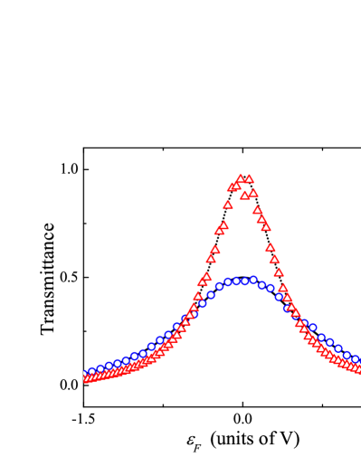
Figure 1: (Color online) Decoherent transmittances obtained for two values of the decoherence strength. For $\Gamma_{\phi}/V=0.01$, the Büttiker transmittance is plotted with the short-dot line and the transmittance of the QD model is plotted with the red triangles for a number $N_{S}=5$ of realizations in the average. For $\Gamma_{\phi}/V=0.3$, the Büttiker transmittance is showed by the solid line and the QD result, with the blue circles for a number of $N_{S}=50$ realizations. The other parameters are: $V=1$, $E_{0}=0$, $V_{L}=V_{R}=0.15$, $E_{r}=0$

The QD method fits the theoretical values to the desired precision. The only difference that one might notice in certain specific cases, such as narrow peaks, would arise from the fact that wave packets are built from states within an energy range as a consequence of the uncertainty principle. On the other hand, scattering theory, by using asymptotic plane waves, has no energy uncertainty. This example is representative of a wide variety of steady state problems that can be solved with the QD method, at only the cost of numerical resources. Indeed, we tested QD on extended systems, a situation where an implementation of the QJ would impose excessive local fluctuations. We found that in QD, much as in quantum parallelism ADLP07 , the collective observables have a tendency to self-average. This makes our model a very promising tool to evaluate decoherent dynamics in extended systems and in many-body problems. However, the true advantage of QD starts to be appreciated in addressing time-dependent problems, as we do in the next section.

V Quantum Dynamical Phase Transition in a Two Level System.

Let us consider a two-level system (TLS) that describes charge or spin dynamics, DALP07(ssc) ; SKVCirGi14 say states $\left|0\right\rangle$ $\equiv$ $\left|\uparrow\downarrow\right\rangle=\hat{c}_{0}^{+}\left|vacuum\right\rangle$ and $\left|1\right\rangle\equiv$ $\left|\downarrow\uparrow\right\rangle=\hat{c}_{1}^{+}\left|vacuum\right\rangle$, with degenerate energy $E_{0}$ and an interaction $V$ mixing them. Such simple system was seen to have a non-trivial dynamics when one of its levels interacts with an environment of spins: a quantum dynamical phase transition (QDPT) ADLP06 . In a QDPT certain observables present a non-analytic dependence on the system-environment interaction strength. The QDPT was missed in a solution for the density matrix in the usual secular approximation of the Redfield theory MKBE74 but showed up in a QJ variant ADLP06 . When the TLS suffers the asymmetric interaction of an environment, the QDPT already appears in the spectrum of the effective non-Hermitian Hamiltonian Rot09 . However, if the interaction is symmetrical, the QDPT only occurs in the density matrix if positivity is ensured P2007PhysB . Thus, obtaining the QDPT in a model with symmetric interaction with the environment constitutes a definitive test for the QD method.

The Hamiltonian of the TLS is

$$\hat{H}_{0}=E_{0}(\hat{c}_{0}^{+}\hat{c}_{0}+\hat{c}_{1}^{+}\hat{c}_{1})-V(\hat{c}_{1}^{+}\hat{c}_{0}+\hat{c}_{0}^{+}\hat{c}_{1}).$$ (13)

The survival probability of an excitation with an initial state $\left|\psi\left(0\right)\right\rangle=\left|0\right\rangle$, i.e. the diagonal element of the density matrix, is

$$P_{00}(t) = \left|\left\langle 0\right|e^{-\mathrm{i}\widehat{H}_{0}t/\hbar}\left|0\right\rangle\right|^{2},$$ (14)

$$= 1/2+1/2\cos\omega_{0}t.$$ (15)

Here, we can observe that $P_{00}(t)$ has Rabi oscillations Cohen92 with frequency $\omega_{0}=2V/\hbar$ and period $T=\pi\hbar/V$.

Let us consider now an environment that interacts independently with each state with a rate described by the Fermi golden rule $1/\tau_{SE}=2\Gamma_{\phi}/\hbar$, where, $\Gamma_{\phi}$ is the energy uncertainty of the level. Physical implications of this model are discussed in the next section in the context of a spin system. The numerical evolution of the TLS is now performed by choosing $\Gamma_{\phi}$ as the width of the Lorentzian distribution.

Here we will compare our QD method, where the decoherent survival probability is

$$\tilde{P}_{00}(t)=\left|\left\langle 0\right|\prod_{n=1}^{N_{t}}e^{-\mathrm{i}\hat{\Sigma}_{n}\mathrm{d}t/\hbar}e^{-\mathrm{i}\widehat{H}_{0}\mathrm{d}t/\hbar}\left|0\right\rangle\right|^{2},$$ (16)

with the analytic solution of the GLBE. This last was analytically solved for this problem in Refs. GLBE1 ; ADLP06 ; P2007PhysB , giving for the survival probability

$$\tilde{P}_{00}(t)=\frac{1}{2}+\frac{1}{2}e^{-\Gamma_{\phi}t/\hbar}\left[\cos\left(\omega t\right)+\frac{\Gamma_{\phi}}{2\omega}\sin\left(\omega t\right)\right].$$ (17)

Thus, the oscillations of both the diagonal and non-diagonal elements of the density matrix oscillate with a frequency $\omega$, which is lower than the Rabi frequency $\omega_{0}$ according to

$$\omega=\sqrt{\omega_{o}^{2}-\left(\Gamma_{\phi}/\hbar\right)^{2}}.$$ (18)

This evidences that the oscillation frequency of a TLS exhibits a non-analytic behavior. The frequency $\omega$ takes real values provided that $\Gamma_{\phi}/\hbar<\omega_{o}$ (underdamped regime). Beyond this value, i.e., for $\Gamma_{\phi}/\hbar>\omega_{o}$ (overdamped regime), $\mathit{Re}(\omega)\equiv 0$ and thus the oscillations are fully suppressed, and $\tilde{P}_{00}(t)$ is the sum of two exponential decays:

$$\tilde{P}_{00}(t)=\frac{1}{2}-\frac{\gamma_{2}}{2(\gamma_{1}-\gamma_{2})}e^{-\gamma_{1}t}+\frac{\gamma_{1}}{2(\gamma_{1}-\gamma_{2})}e^{-\gamma_{2}t},$$ (19)

where the decay rate $\gamma_{1(2)}$ is

$$\gamma_{1(2)}=\frac{1}{\hbar}\left(\Gamma_{\phi}\pm\sqrt{\Gamma_{\phi}^{2}-(\hbar\omega_{o})^{2}}\right).$$ (20)

Note that, at short times, $\tilde{P}_{00}(t)$ is always of the form $1-\omega_{o}^{2}t^{2}/4=1-V^{2}t^{2}/\hbar^{2}$, which is characteristic of a quantum evolution without perturbations. This is because, at short times, the environment interplay has a small cumulative effect on the survival probability, which is still determined by the unperturbed quantum dynamics. In a strongly decoherent regime, $\Gamma_{\phi}/\hbar\gg\omega_{o}$, the decay rates tend to $\gamma_{1}\simeq 2\Gamma_{\phi}/\hbar$, $\gamma_{2}\simeq\hbar\omega_{o}^{2}/2\Gamma_{\phi}$, defining a short-time decay rate, $\gamma_{1}$, and a rate $\gamma_{2}$, that dominates the long times as $\tilde{P}_{00}(t)\propto e^{-\gamma_{2}t}$. Both exponential terms are needed to obtain the whole evolution. An equivalent solution for the QDPT may be obtained by considering models for environmental noise Altshuler14 .

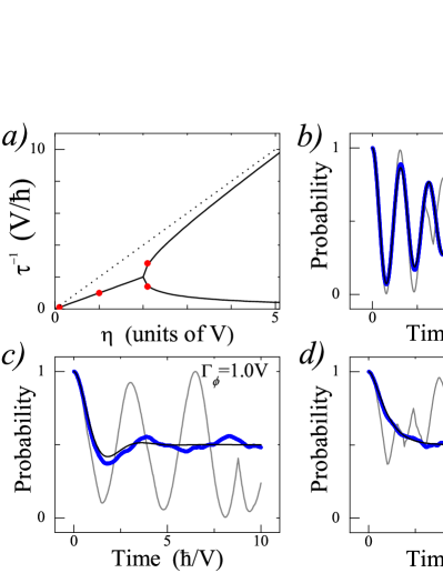
Figure 2: (Color online) $(a)$ Theoretical rates of decay predicted by the Eqs. 17 and 20. Red points indicate the rates of the GLBE solution for $(b)-(d)$. The QDPT occurs as a bifurcation in the rates for the critical value $\Gamma_{\phi}/V=2$. The dotted line represents the asymptotic value $2\Gamma_{\phi}/\hbar$. In $(b)-(d)$, we show the survival probabilities $\tilde{P}_{00}(t)$ (thick blue line), the GLBE solutions (thin black line), and individual realizations (thin gray line) in the underdamped regime, in $(b)$ with $\Gamma_{\phi}/V=0.1$ and $(c)$ with $\Gamma_{\phi}/V=1$, and in the overdamped regime, $(d)$ with $\Gamma_{\phi}/V=2.1$. Individual realizations tend to preserve the oscillations. These do not have jumps in the densities but in the slopes. The ensemble average is taken over $N_{S}=100$ realizations. For $\tilde{P}_{00}(t)\simeq 1/2$ are clear the typical fluctuations of the order of $1/\sqrt{N_{S}}$. The average $\tilde{P}_{00}(t)$ tends to the GLBE solution by increasing $N_{S}$.

In Fig. 2$(a)$ the decay rates are shown. The QDPT is manifested as the bifurcation in these rates. The fitted rates are shown as points superposed to the theoretical curve. In Fig. 2$(b)$, we show the Rabi oscillations of the average survival probability, $\tilde{P}_{00}(t)$, which are exponentially attenuated with $\tau^{-1}\simeq\Gamma_{\phi}/\hbar=1/2(\tau_{SE})^{-1}$. This is the most common example of decoherence in TLS’s. The $\tilde{P}_{00}(t)$ and the fitted decay rates match perfectly the GLBE solution. A single realization of QD method is also shown. Notice that there are no “jumps” in the survival probability, and an oscillatory-like behavior dominates the whole evolution. In Fig. 2$(c)$ we show the $\tilde{P}_{00}(t)$ in the underdamped regime for a value of $\Gamma_{\phi}=1V$, where, the oscillatory behavior is small. In Fig. 2$(d)$ we show $\tilde{P}_{00}(t)$ in the overdamped regime, for $\Gamma_{\phi}=2.1V$. We can identify the initial quadratic behavior and, at large times, the exponential decay with the rate $\gamma_{2}\propto 1/\Gamma_{\phi}$. The larger $\Gamma_{\phi}$, the slower $\tilde{P}_{00}(t)$ decays. This is a signature of the quantum Zeno effect in which the system is continuously perturbed freezing its evolution close to the initial condition. By increasing $\Gamma_{\phi}$, each single realization seems to be a stochastic process while preserving the quadratic initial starting. Single realizations do not present jumps in the density but in the correlations, seen as sudden changes on the slopes.

The actual dynamics of the observables emerge after ensemble averaging. As long as the survival probability is not too close to $1/2$, a fair representation of $\tilde{P}_{00}(t)$ is obtained with about $N=100$ realizations as shown in Fig. 2. Strongly damped cases evidence the typical fluctuations of random numbers where the observables have a precision of $1/\sqrt{N}$. In these cases, individual systems maintain a substantial oscillation whose slopes can be strongly discontinuous. Thus to obtain coincidence with the exact theoretical values within the graphical resolution (say $1\%$) one needs about $N=10\ 000$ realizations. We tested a binary and Gaussian phase drift distributions and the fluctuations and their influence on the precision of the ensemble averages persist. However, this is hardly a limitation if one is still far from the asymptotic values or when one addresses global observables.

VI Quantum Jumps vs. Quantum Drift in a many-spin dynamics

Here, we will further assess the differences between the QJ and QD in a situation of actual experimental relevance where the density matrix approach is clearly restrictive: that of many-spin dynamics. We will address the decoherent dynamics of this problem, which is non-trivial in terms of the density matrix. We are interested in the dynamics of a local spin excitation in a system of $M$ interacting spins $1/2$. Let us say that the state at $t=0$ is given by the density matrix:

$$\hat{\rho}_{0}=\frac{1}{2^{M}}(\mathbf{\hat{I}}+2\hat{S}_{1}^{z}),$$ (21)

which describes that spin $1$ is up-polarized. At very high temperature the other spins are not polarized at all, i.e. $tr[\hat{S}_{1}^{z}\hat{\rho}_{0}]=\frac{1}{2}$ and $tr[\hat{S}_{i}^{z}\hat{\rho}_{0}]=0$ $\forall i\neq 1$. In order to be more specific, let us consider the particular case of a linear chain with $M=5$ that was addressed theoretically and experimentally in NMR and where a decoherent calculation is lacking Ernst97 ; Past96CPL ; P95PRL . There, the effective Hamiltonian is reduced to nearest-neighbors planar (or $XY$) interactions. The Hamiltonian, using the spin lowering $\hat{S}_{i}^{-}$ and raising $\hat{S}_{i}^{+}$ operators is:

$$\hat{H}_{chain} = \sum_{i=1}^{M-1}J_{i,i+1}(\hat{S}_{i}^{+}\hat{S}_{i+1}^{-}+\hat{S}_{i+1}^{+}\hat{S}_{i}^{-})$$ (22)

$$+\sum_{i=1}^{M}\hbar\Omega_{i}(\hat{S}_{i}^{+}\hat{S}_{i}^{-}-\frac{1}{2}).$$

The first term is the $XY$ Hamiltonian, accounting for the couplings to nearest-neighbours. We will take $J_{i,i+1}=J$ as the unit of energy. The second one is the Zeeman Hamiltonian, where the precession frequencies are $\Omega_{i}=\omega_{0}$, and $\omega_{0}$ is the Larmor frequency in the external magnetic field. As predicted by the coherent calculation, the local excitation $\hat{\rho}_{0}$ was seen to propagate as a spin wave through the molecular chain and returns to the initial site in the form of a mesoscopic echo (ME). It is precisely the wave packet behavior that makes these systems promising as quantum channels CRC07 ; Bose03 ; CrisDEL07 ; Zwick11 . However, the experiments show that these spin waves decohere and attenuate as time pass by. Thus, here we consider that each spin is perturbed by a local environment that acts as a fluctuating Zeeman field. Thus $\Omega_{i}=\omega_{0}+\delta\omega_{i}$, where $\delta\omega_{i}$ fluctuates with time.

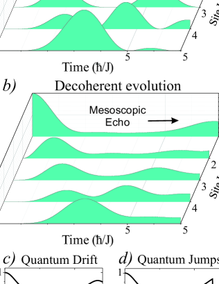
Figure 3: (Color online) Density as function of time at each spin for $(a)$ the coherent evolution, $(b)$ an average evolution with a finite coherence time $T_{coh}=3\hbar/J$, $(c)$ a single realization of the QD model, and $(d)$ a single realization of the QJ model. When the spin wave reaches the edge of the chain, it is reflected constituting the mesoscopic echo. Note that the curves for QD are smooth in density whereas those for QJ present a sudden change when the jump is produced.

We will solve this problem by resorting the Jordan-Wigner transformation DPL02PhysB which in this case looks $\hat{S}_{i}^{+}\longleftrightarrow\hat{c}_{i}^{+}$, $\hat{S}_{i}^{-}\longleftrightarrow\hat{c}_{i}$ and $\hat{S}_{i}^{z}\longleftrightarrow\hat{c}_{i}^{+}\hat{c}_{i}-1/2$ . Thus, this many-spin system can be reduced to a one-body problem. This transformation remains valid when considering the random fluctuations in the Zeeman field. Then, it is clear that these produce local energy fluctuations $\hbar\delta\omega_{i}$ that show up as decoherence in the spin dynamics. Note that the fluctuations are naturally described within the QD prescription and, conversely, the random phases of QD have a direct physical meaning in this problem.

In Figs. 3$(a)$ and 3$(b)$ we compare the coherent and decoherent evolutions of the spin wave. The local excitation travels from site $1$ to the edge of the chain and there it is reflected and returns to the initial spin as a ME. We use a decoherence time of about $\ 3\hbar/J$, consistent with the experimental observation.Ernst97 In Figs. 3$(c)$ and 3$(d)$ we show the local density for a single realization for both the QD and QJ methods. The QD has a smoother profile whereas the QJ resembles the coherent evolution until the jump is produced.

In similar problems, the master equation for the density matrix could be used to obtain the decoherent dynamics ZnidHv13 . However, with regard to numerical calculations, it is very demanding. Thus, the QJ method, which is based on a stochastic wave function, has proved to be more convenient in addressing large systems. Petr97 Indeed, it is faster and less demanding to perform an average over many realizations of the QJ than computing the whole density matrix. Since our QD method is also based in a stochastic wave function, for large enough systems the QD must become more convenient than a density matrix approach. Thus, we shall compare the QD with the QJ.

We will look at the convergence to the average decoherent dynamics for both QJ and QD methods. Due to the discontinuous nature of QJ, we expect that the difference with the mean dynamics is greater for QJ than for QD (see Figs. 3$(c)$ and 3$(d)$). This can be quantified in terms of the time average of the standard error,

$$\sigma^{(QD,QJ)}=\sqrt{\frac{1}{N_{s}~{}T}\int_{0}^{T}\mathrm{d}t\sum_{i=1}^{N_{s}}\left(\rho_{i,i}^{(QD,QJ)}(t)-\bar{\rho}_{i,i}(t)\right)^{2}}.$$ (23)

Here, $T$ is the evolution time and $\bar{\rho}_{ii}(t)=\overline{\left|i\right\rangle\left\langle i\right|}$ is the mean density at time $t$ at site $i$ obtained from an average over $N_{s}=10^{5}$ realizations, where both QJ and QD converge to the the same average dynamics with negligible error. In Fig. 4 we show $\sigma N_{s}^{1/2}$ for different values of $N_{s}$ as function of the evolution time $T$. Thus, this result evidences the general tendency of the QD method to present a smaller deviation from the mean than the QJ. Indeed, for each $N_{s}$, $\sigma^{QJ}$ is greater than $\sigma^{QD}$ by a factor of almost $2$. Thus, to converge with a given $\sigma$, QD needs to perform roughly the half of realizations than QJ.

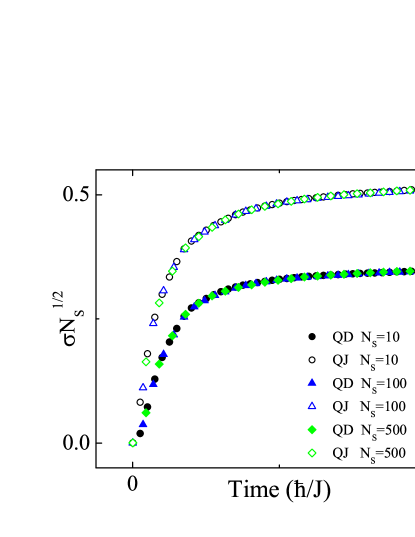
Figure 4: (Color online) The standard error $\sigma$ times $\sqrt{N}_{s}$ as function of the evolution time, for $N_{s}=10,100$, and $500$. Note that $\sigma N_{s}^{1/2}$ does not depends on $N_{s}$ but in the QD or QJ method. Note that, for the same $N_{s}$, $\sigma^{QJ}/\sigma^{QD}\approx 2$.

VII Loschmidt Echo

Following the logic of the two previous sections, one would be tempted to assign the meaning of decoherence to the decay of the oscillations. However, it has been clarified that a way to filter away the intrinsic dynamics from the observable is by using the Loschmidt echo (LE) JalP01 . This is the amount of excitation recovered after a time-reversal procedure implemented in presence of an environment. The advantage is that the LE codifies in a local observable the losses of non-local correlations. As in NMR experiments, this consists in changing the sign of the acting Hamiltonian $\widehat{H}_{0}\longrightarrow-\widehat{H}_{0}$. By using the Trotter-Suzuki expansion, the LE can be defined as:

$$M_{00}(2t) = \left|\left\langle 0\right|\prod_{m=N_{t}+1}^{2N_{t}}e^{+\mathrm{i}\widehat{H}_{0}\mathrm{d}t/\hbar}e^{-\mathrm{i}\hat{\Sigma}_{m}\mathrm{d}t/\hbar}\right.\times$$ (24)

$$\left.\prod_{n=1}^{N_{t}}e^{-\mathrm{i}\hat{\Sigma}_{n}\mathrm{d}t/\hbar}e^{-\mathrm{i}\widehat{H}_{0}\mathrm{d}t/\hbar}\left|0\right\rangle\right|^{2}$$

where $N_{t}=t/\mathrm{d}t$, and $\hat{\Sigma}_{n}$ is the perturbation’s Hamiltonian. Note that, whereas the sign of the Hamiltonian changes, the perturbation remains with the same sign.

In Fig. 5$(a)$, we show the survival probability $\widetilde{P}_{00}(t)$ and the Loschmidt echo $M_{00}(t)$ in the underdamped regime as function of the time of interaction with the environment, $t$. Surprisingly, in the underdamped regime, $M_{00}$ is not a simple exponential but has plateaus whenever the reversal starts while the system is at $\left|0\right\rangle$ or $\left|1\right\rangle$. On the contrary, $M_{00}$ suffers a maximal decay if the reversal starts when the system is at a superposition state $\left[\left|0\right\rangle\pm\left|1\right\rangle\right]/\sqrt{2}$. When the density is placed on one site, decoherent interactions act as a change in the global phase, which does not destroy the phase correlations between $\left|0\right\rangle$ and $\left|1\right\rangle$. Notice that the homogeneous exponential decay of the survival probability does not discriminate on the initial state, while the LE does. In any case, if one should define a overall rate $\gamma_{\phi LE}\equiv 1/\tau_{\phi LE}$ from the LE, it would coincide with that observed in the oscillation decay, i.e., $\gamma_{\phi LE}\simeq\Gamma_{\phi}/\hbar=1/2(\tau_{SE})^{-1}$. Thus, the LE gives a rationale to the $1/2$ factor: decoherent processes are effective on one half of the dynamical cycle.

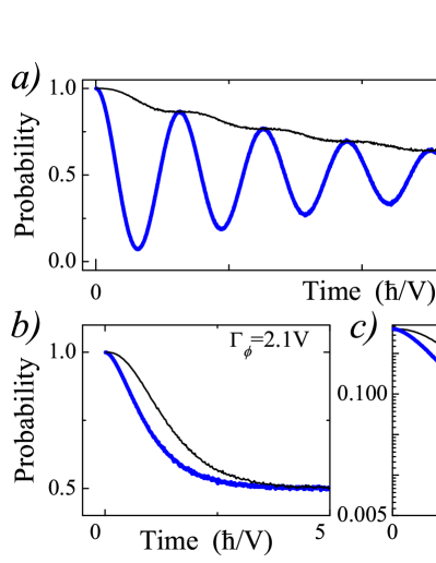
Figure 5: (Color online) Survival probability (thick blue line) and the Loschmidt echo (thin black line) as function of the time of action of the environment for: $(a)$ $\eta/V=0.1$ and $(b)$ $\eta/V=2.1$, averaged over $N_{S}=10000$ realizations. $(c)$: the same as in $(b)$ but in log scale. The rate of decay of the LE, $1/\tau_{SE}=1.12V/\hbar$, is smaller than the minimum decay rate of the $\tilde{P}_{00}$, $1/\tau_{2}=1.46V/\hbar$.

The overdamped regime is shown in Fig. 5$(b)$ and in a log scale in Fig. 5$(c)$ . This last clarifies the different decay rates and the difficulties to obtain probabilities around 1/2 from a limited number of realizations. The LE has a wider plateau than the survival probability at short times. For the same period of action of the decoherent processes, the LE signal is higher than the survival probability. This fact is consistent with that, in order for decoherent processes to be effective, the dynamics must first build up the superposition state. The decay rate of the LE does not fit with Eq. 20. By using a single exponential, the decay rate is $1/\tau_{\phi LE}=1.12V/\hbar$, which is slightly smaller than the minimum rate of $\tilde{P}_{00}$, $\gamma_{2}=\Gamma_{\phi}-\sqrt{\Gamma_{\phi}^{2}-(\hbar\omega_{o})^{2}}=1.46V$. This indicates that the LE gives more weight to the less correlated short-time processes where the strong interaction with the environment does not allow us to create the correlations and thus, it should have a slower decay.

VIII Final Discussion

We developed and implemented a stochastic model to include decoherent processes in quantum dynamics. Inspired in the Büttiker-D’Amato-Pastawski description of decoherent transport, it boils down to a wave function that undergoes smooth stochastic drifts in a local basis.

Unlike the quantum jumps (QJ) approach, no collapses of the wave function occur and phase shifts are introduced in a unitary dynamics. Thus, in QD jumps can only appear in the correlations functions, not in the local densities. Being an appealing conceptual framework, with a clear physical meaning, our QD model results particularly adapted to deal with extended system. Besides, it admits further extensions, ranging from the evaluation of currents in transport set-ups to the representation of specific many-body interactions.

Using numerical calculations, we proved that our dynamical model is in a full agreement with the decoherent-steady-state conductances through the resonant state $\left|0\right\rangle$ of a decoherent quantum dot, even resorting to a quite restricted ensemble average. For steady-state transport in extended systems, a QD evaluation of the wave function is, by construction, more efficient than density matrix approaches ZnidHv13 .

In spin systems, the physical foundation of the QD model becomes evident. Decoherence associated to the fluctuation of the local energy is a natural ingredient associated with the fast fluctuation of the local Zeeman fields. Thus, we tested the dynamical properties of QD model by applying it to a two-spin system and a five spin system in presence of decoherence. The first is a two-level system (TLS) that oscillates among $\left|0\right\rangle$ $\equiv$ $\left|\uparrow\downarrow\right\rangle$ and $\left|1\right\rangle\equiv$ $\left|\downarrow\uparrow\right\rangle$. There, a non-trivial quantum dynamical phase transition shows up, which was observed in NMR and obtained from the solution of the generalized Landauer-Büttiker equations ADLP07 ; DALP07(ssc) . We recovered not only the exponential damping of the oscillations at low rates of interaction with the environment but also the bifurcation of the decoherence rates at a critical interaction strength. The evaluation of the decoherent dynamics of a five-spin system is also done in connection with NMR experiments Ernst97 . By using rates consistent with the experiment, we show the robustness of the mesoscopic echo under decoherence. We also show that, for a given tolerance error for an observable, the QD method demands about half the realizations than QJ.

By evaluating decoherence in the TLS through Loschmidt echo (LE), we found that the pure states $\left|0\right\rangle$ $\equiv$ $\left|\uparrow\downarrow\right\rangle$ and $\left|1\right\rangle\equiv$ $\left|\downarrow\uparrow\right\rangle$ are quite robust against local perturbations of the environment. In contrast, the LE, and hence coherence, decays faster when the system is in a superposition state $\left(\left|\uparrow\downarrow\right\rangle\pm\left|\downarrow\uparrow\right\rangle\right)/\sqrt{2}$. These results are in agreement with the general trend recently observed in spin systems through NMR Sanchez14 .

In summary, we proposed a QD model that provides a stochastic unitary dynamics of the wave function. Observable evaluation of observables through QD and QJ are naturally parallelizable and thus they result in being more scalable than density matrix methodsPetr97 . This quality, which adds to the intrinsic physical significance, should make the QD method a suitable tool to address dynamical observables in both extended one-body and many-body systems.

- (1) I. Bloch, “Quantum gases in optical lattices,” Phys. World, vol. 17, p. 25, 2004.
- (2) J. I. Cirac and P. Zoller, “New frontiers in quantum information with atoms and ions,” Phys. Today, vol. 57, p. 38, 2004.
- (3) P. Cappellaro, C. Ramanathan, and D. G. Cory, “Simulations of information transport in spin chains,” Phys. Rev. Lett., vol. 99, p. 250506, 2007.
- (4) W. Lu, Z. Ji, L. Pfeiffer, K. W. West, and A. J. Rimberg, “Real-time detection of electron tunnelling in a quantum dot,” Nature (London), vol. 423, pp. 422–425, 2003.
- (5) M. J. A. Schuetz, E. M. Kessler, L. M. K. Vandersypen, J. I. Cirac, and G. Giedke, “Nuclear spin dynamics in double quantum dots: Multistability, dynamical polarization, criticality, and entanglement,” Phys. Rev. B, vol. 89, p. 195310, 2014.
- (6) J. R. Petta, A. C. Johnson, J. M. Taylor, E. A. Laird, A. Yacoby, M. D. Lukin, C. M. Marcus, M. P. Hanson, and A. C. Gossard, “Coherent manipulation of coupled electron spins in semiconductor quantum dots,” Science, vol. 309, p. 2180, 2005.
- (7) G. Lindblad, “On the generators of quantum dynamical semigroups,” Commun. Math. Phys., vol. 48, p. 119, 1976.
- (8) A. Kossakowski, “On quantum statistical mechanics of non- hamiltonian systems,” Rep. Math. Phys., vol. 3, p. 247, 1972.
- (9) A. Redfield, “The theory of relaxation processes,” Adv. Magn. Res., vol. 1, p. 1, 1965.
- (10) C. P. Slichter, Principles of Magnetic Resonance. Springer, 1996.
- (11) J. Dalibard, Y. Castin, and K. Mølmer, “Wave-function approach to dissipative processes in quantum optics,” Phys. Rev. Lett., vol. 68, pp. 580–583, 1992.
- (12) K. Mølmer, Y. Castin, and J. Dalibard, “Monte carlo wave-function method in quantum optics,” J. Opt. Soc. Am. B, vol. 10, p. 524, 1993.
- (13) W. G. Teich and G. Mahler, “Stochastic dynamics of individual quantum systems: Stationary rate equations,” Phys. Rev. A, vol. 45, p. 3300, 1992.
- (14) H. J. Carmichael, S. Singh, R. Vyas, and P. R. Rice, “Photoelectron waiting times and atomic state reduction in resonance fluorescence,” Phys. Rev. A, vol. 39, pp. 1200–1218, 1989.
- (15) H. J. Carmichael, “Quantum trajectory theory for cascaded open systems,” Phys. Rev. Lett., vol. 70, pp. 2273–2276, 1993.
- (16) H. P. Breuer, W. Huber, and F. Petruccione, “Stochastic wave-function method versus density matrix: a numerical comparison,” Comput. Phys. Commun., vol. 104, p. 46, 1997.
- (17) B. L. Altshuler and A. G. Aronov, Electron-Electron Interactions in Disordered Systems, edited by M. Pollack and A. I. Efros (North-Holland, Amsterdan, 1985).
- (18) D. J. Thouless, “Electrons in disordered systems and the theory of localization,” Phys. Rep., vol. 13, no. 3, p. 93, 1974.
- (19) Y. Imry and R. Landauer, “Conductance viewed as transmission,” Rev. Mod. Phys., vol. 71, p. S306, 1999.
- (20) M. Büttiker, “Role of quantum coherence in series resistors,” Phys. Rev. B, vol. 33, pp. 3020–3026, 1986.
- (21) J. L. D’Amato and H. M. Pastawski, “Conductance of a disordered linear chain including inelastic scattering events,” Phys. Rev. B, vol. 41, p. 7411, 1990.
- (22) H. M. Pastawski, “Classical and quantum transport from generalized landauer-büttiker equations,” Phys. Rev. B, vol. 44, pp. 6329–6339, Sep 1991.
- (23) N. A. Zimbovskaya and G. Gumbs, “On the low frequency electromagnetic waves in quasi-two-dimensional metals,” Solid State Commun., vol. 146, no. 1–2, pp. 88 – 91, 2008.
- (24) D. Nozaki, C. Gomes da Rocha, H. M. Pastawski, and G. Cuniberti, “Disorder and dephasing effects on electron transport through conjugated molecular wires in molecular junctions,” Phys. Rev. B, vol. 85, p. 155327, 2012.
- (25) C. J. Cattena, L. J. Fernández-Alcázar, R. A. Bustos-Marún, D. Nozaki, and H. M. Pastawski, “Generalized multi-terminal decoherent transport: recursive algorithms and applications to saser and giant magnetoresistance,” J. Phys.: Condens. Matter, vol. 26, no. 34, p. 345304, 2014.
- (26) H. M. Pastawski, “Classical and quantum transport from generalized landauer-büttiker equations. ii. time-dependent resonant tunneling,” Phys. Rev. B, vol. 46, pp. 4053–4070, Aug 1992.
- (27) P. Myöhänen, A. Stan, G. Stefanucci, and R. van Leeuwen, “Kadanoff-baym approach to quantum transport through interacting nanoscale systems: From the transient to the steady-state regime,” Phys. Rev. B, vol. 80, p. 115107, 2009.
- (28) E. Khosravi, A.-M. Uimonen, A. Stan, G. Stefanucci, S. Kurth, R. van Leeuwen, and E. K. U. Gross, “Correlation effects in bistability at the nanoscale: Steady state and beyond,” Phys. Rev. B, vol. 85, p. 075103, 2012.
- (29) G. A. Álvarez, E. P. Danieli, P. R. Levstein, and H. M. Pastawski, “Decoherence under many-body system-environment interactions: A stroboscopic representation based on a fictitiously homogenized interaction rate,” Phys. Rev. A, vol. 75, p. 062116, 2007.
- (30) E. Danieli, G. Álvarez, P. Levstein, and H. Pastawski, “Quantum dynamical phase transition in a system with many-body interactions,” Solid State Commun., vol. 141, no. 7, pp. 422 – 426, 2007.
- (31) G. A. Álvarez, E. P. Danieli, P. R. Levstein, and H. M. Pastawski, “Quantum parallelism as a tool for ensemble spin dynamics calculations,” Phys. Rev. Lett., vol. 101, p. 120503, 2008.
- (32) G. A. Álvarez, E. P. Danieli, P. R. Levstein, and H. M. Pastawski, “Environmentally induced quantum dynamical phase transition in the spin swapping operation,” J. Chem. Phys., vol. 124, no. 19, p. 194507, 2006.
- (33) R. A. Jalabert and H. M. Pastawski, “Environment-independent decoherence rate in classically chaotic systems.,” Phys. Rev. Lett., vol. 86, p. 2490, 2001.
- (34) H. M. Pastawski and E. Medina, “Tight binding methods in quantum transport trough molecules and small devices: from the coherent to the decoherent description,” Rev. Mex. Fis., vol. 47, p. 1, 2001.
- (35) An explicit evaluation of the energy dependence of shows that attenuation is not much effective for the small off-resonance tunneling, as the electrons with energies away from the resonance spent a very short time at this interacting state.
- (36) L. Müller, A. Kumar, T. Baumann, and R. R. Ernst, “Transient oscillations in nmr cross-polarization experiments in solids,” Phys. Rev. Lett., vol. 32, p. 1402, 1974.
- (37) I. Rotter, “A non-hermitian hamilton operator and the physics of open quantum systems,” J. Phys. A: Math. Theor., vol. 42, no. 15, p. 153001, 2009.
- (38) H. Pastawski, “Revisiting the fermi golden rule: Quantum dynamical phase transition as a paradigm shift.,” Physica B, vol. 398, p. 278, 2007.
- (39) C. Cohen-Tannoudji, G. Grynberg, and J. Dupont-Roc, Atom-Photon Interactions: Basic Processes and Applications. Wiley, 1992.
- (40) E. Paladino, Y. M. Galperin, G. Falci, and B. L. Altshuler, “ noise: Implications for solid-state quantum information,” Rev. Mod. Phys., vol. 86, pp. 361–418, 2014.
- (41) Z. L. Mádi, B. Brutscher, T. Schulte-Herbrüggen, R. Brüschweiler, and R. R. Ernst, “Time-resolved observation of spin waves in a linear chain of nuclear spins,” Chem. Phys. Lett., vol. 268, p. 300, 1997.
- (42) H. M. Pastawski, G. Usaj, and P. R. Levstein, “Quantum interference phenomena in the local polarization dynamics of mesoscopic systems: an nmr observation,” Chem. Phys. Lett., vol. 261, p. 329, 1996.
- (43) H. Pastawski, P. Levstein, and G. Usaj, “Quantum dynamical echoes in the spin diffusion in mesoscopic systems,” Phys. Rev. Lett., vol. 75, p. 4310, 1995.
- (44) S. Bose, “Quantum communication through an unmodulated spin chain,” Phys. Rev. Lett., vol. 91, p. 207901, 2003.
- (45) M. Christandl, N. Datta, A. Ekert, and A. J. Landahl, “Perfect state transfer in quantum spin networks,” Phys. Rev. Lett., vol. 92, p. 187902, 2004.
- (46) A. Zwick, G. A. Alvarez, J. Stolze, and O. Osenda, “Robustness of spin-coupling distributions for perfect quantum state transfer,” Phys. Rev. A, vol. 84, p. 022311, 2011.
- (47) E. Danieli, H. Pastawski, and P. Levstein, “Exact spin dynamics of inhomogeneous 1-d systems at high temperature,” Physica B, vol. 320, p. 351, 2002.
- (48) M. Žnidarič and M. Horvat, “Transport in a disordered tight-binding chain with dephasing,” Eur. Phys. J. B, vol. 86, no. 2, pp. 1–11, 2013.
- (49) C. M. Sánchez, R. H. Acosta, P. R. Levstein, H. M. Pastawski, and A. K. Chattah, “Clustering and decoherence of correlated spins under double quantum dynamics,” Phys. Rev. A, vol. 90, p. 042122, Oct 2014.