Analytical formula for numerical evaluations of the Wigner rotation matrices at high spins

Abstract

The Wigner $d$ function, which is the essential part of an irreducible representation of SU(2) and SO(3) parameterized with Euler angles, has been know to suffer from a serious numerical errors at high spins, if it is calculated by means of the Wigner formula as a polynomial of cos and sin of half of the second Euler angle. This paper shows a way to avoid this problem by expressing the $d$ functions as the Fourier series of the half angle. A precise numerical table of the coefficients of the series is provided as Supplemental Material.

I Introduction

The matrix elements of the rotation operator between angular-momentum eigenstates are called the Wigner $D$ function Rose (1957). When the rotation is specified with the three Euler angles ($\phi$, $\theta$, $\psi$), and the eigenstates are labeled with the magnitude ($j$ = $0,\frac{1}{2},1,\frac{3}{2},\cdots$) and the $z$ component ($m$ or $k$ = $-j,-j+1,\cdots,j$) of the angular momentum vector, the $D$ function can be decomposed into three factors,

$$D^{j}_{mk}(\phi,\theta,\psi) = \langle jm|e^{-i\phi\hat{j}_{z}}e^{-i\theta\hat{j}_{y}}e^{-i\psi\hat{j}_{z}}|jk\rangle$$ (1)

$$= e^{-i(m\phi+k\psi)}d^{j}_{mk}(\theta),$$

where

$$d^{j}_{mk}(\theta)=\langle jm|e^{-i\theta\hat{j}_{y}}|jk\rangle$$ (2)

is the nontrivial part which needs some method to evaluate. It is called the Wigner (small) $d$ function. In the standard phase convention for angular-momentum eigenstates, the matrix elements of $\hat{j}_{y}$ are purely imaginary and thus $d^{j}_{mk}(\theta)$ takes on real numbers.

One may be anxious about the fact that Bohr and MottelsonBohr and Mottelson (1969) define the rotation matrix $D^{j}_{mk}$ as the complex conjugate of the right-hand side (r.h.s.) of Eq.(1). However, their definition for $d^{j}_{mk}$ is identical with Wigner’s and the definition of the $d$ function is unique.

The Wigner $D$ function is used in various fields of physics. In some applications, those for large values of $j$ (say, $>50$) are necessary. An example in nuclear structure physics is the projection from spatially deformed solutions of modern realistic mean-field models to eigenstates of large angular momentum. For toy models, too, one occasionally needs $d$ functions for very large $j$ to confirm the validity of one’s picture under extreme conditions. (e.g., a two-rotor model of Refs. Tajima (2013) and Tajima and Otsuka (2011)).

The explicit form of the $d$ function is given by the Wigner formulaRose (1957), which can be written as,

$$d^{j}_{mk}(\theta)=\sum_{n=n_{\rm min}}^{n_{\rm max}}(-1)^{n}W_{n}^{jmk}(\theta),$$ (3)

where $n_{\rm min}$ and $n_{\rm max}$ are zero or positive integers,

$$n_{\rm min} = \max(0,k-m),$$ (4)

$$n_{\rm max} = \min(j-m,j+k),$$ (5)

and

$$W_{n}^{jmk}(\theta)=w_{n}^{jmk}\cdot\left(\cos{\textstyle\frac{\theta}{2}}\right)^{2j+k-m-2n}\left(-\sin{\textstyle\frac{\theta}{2}}\right)^{m-k+2n},$$ (6)

$$w_{n}^{jmk}=\frac{\sqrt{(j+m)!(j-m)!(j+k)!(j-k)!}}{(j-m-n)!(j+k-n)!(n+m-k)!n!}.$$ (7)

However, this formula suffers from a serious loss of precision at high spins (i.e., for large $j$) except in the neighborhood of $\theta=0,\pi$.

For example, assuming that $j$ is a positive integer, $\theta=\frac{\pi}{2}$, and $m=k=0$, one obtains

$$W_{n}^{j00}\left(\frac{\pi}{2}\right)=\frac{1}{2^{j}}\left[\frac{j!}{(j-n)!n!}\right]^{2},$$ (8)

which, if $j$ is even, becomes maximum at $n=\frac{j}{2}$,

$$W_{j/2}^{j00}\left(\frac{\pi}{2}\right)=\frac{1}{2^{j}}\frac{j!}{\left[(j/2)!\right]^{2}}\approx\sqrt{\frac{2}{\pi j}}2^{j}.$$ (9)

(The Stirling’s formula is used in the last approximation.) The absolute value of the $d$ function is not greater than one because it is a matrix element of a unitary operator between normalized states. Wigner’s formula expresses the $d$ function as a result of cancellation among terms of possibly huge size, $W_{n}^{jmk}\sim 2^{j}$. For $j\sim 54$, the precision of double-precision floating-point numbers (53-bit mantissa) is lost completely, and even quadruple precision float numbers (113-bit mantissa) is lost completely for $j\sim 114$.

A few remedies have been proposed Choi et al. (1999); Dachsel (2006) but the results are not completely free of the precision loss. In this paper, I investigate the details of this loss of significance, and then present a perfect remedy to avoid such numerical difficulty.

II The Fourier-series expression of $d$ functions

One can see easily that terms like $\cos^{\lambda}\frac{\theta}{2}\sin^{\mu}\frac{\theta}{2}$ appearing in the r.h.s. of Eq. (6), where $\lambda$ and $\mu$ are zero or positive integers such that $\lambda+\mu\leq 2j$, can be expressed as linear combinations of terms $\sin\frac{\kappa\theta}{2}$ (when $\mu$ is odd) and $\cos\frac{\kappa\theta}{2}$ (when $\mu$ is even) with integers $\kappa$ in $0\leq\kappa\leq\lambda+\mu$ and $\kappa\equiv\lambda+\mu$ (mod 2), by means of repeated applications of the elementary trigonometric identities called the product-to-sum identities or the prosthaphaeresis formulas.

Because the power of $\sin\frac{\theta}{2}$ is $\mu=m-k+2n$ in Eq. (6), one can see that $\mu\equiv m-k$ (mod 2) and that the $d$ function is an even (odd) function if $m-k$ is even (odd), which can be expanded only with cos (sin) function. This may also be deduced from Eq. (33), one of the properties of the $d$ function which I have enumerated in the appendix A.

From these considerations, one can conclude that the Fourier expansion of the $d$ function has the following form:

$$d^{j}_{mk}(\theta)=\sum_{\nu}t^{jmk}_{\nu}f(\nu\theta),$$ (10)

where

$$f=\left\{\begin{array}[]{c}\cos\\ \sin\end{array}\right\}\;\;\;\mbox{for}\;\;\left\{\begin{array}[]{c}\mbox{even}\\ \mbox{odd}\end{array}\right\}m-k,$$ (11)

and the summation runs over

$$\nu=\nu_{\rm min},\nu_{\rm min}+1,\cdots,j,$$ (12)

with the values of $\nu_{\rm min}$ given in Table 1.

Table 1: The values of $\nu_{\rm min}$ appearing in Eq. (10)

	Even $m-k$	Odd $m-k$
Even $2j$	0	1
Odd $2j$	$\frac{1}{2}$	$\frac{1}{2}$

For example, for $j=\frac{7}{2}$ and $m=-k=\frac{1}{2}$, the Wigner formula (3) gives an expression,

$$d^{\frac{7}{2}}_{\frac{1}{2},-\frac{1}{2}}(\theta) = \sin^{7}{\textstyle\frac{\theta}{2}}-12\cos^{2}{\textstyle\frac{\theta}{2}}\,\sin^{5}{\textstyle\frac{\theta}{2}}+18\cos^{4}{\textstyle\frac{\theta}{2}}\,\sin^{3}{\textstyle\frac{\theta}{2}}$$ (13)

$$-4\cos^{6}{\textstyle\frac{\theta}{2}}\,\sin{\textstyle\frac{\theta}{2}},$$

which can be rewritten in the form (10) as

$$d^{\frac{7}{2}}_{\frac{1}{2},-\frac{1}{2}}(\theta)=-\frac{35\,\sin{\textstyle\frac{7\theta}{2}}-5\,\sin{\textstyle\frac{5\theta}{2}}+15\,\sin{\textstyle\frac{3\theta}{2}}-9\,\sin{\textstyle\frac{\theta}{2}}}{64}.$$ (14)

By utilizing the orthogonality of $\cos\nu\theta$ and $\sin\nu\theta$ over $0\leq\theta\leq 4\pi$ (considering that $\nu$ can take both integer and half-integer values), one can express the coefficients $t_{\nu}^{jmk}$ by an integral

$$t^{jmk}_{\nu}=\frac{1}{2\pi(1+\delta_{\nu 0})}\int_{0}^{4\pi}d^{j}_{mk}(\theta)f(\nu\theta)d\theta,$$ (15)

where $\delta_{\nu 0}=1$ for $\nu=0$ and $\delta_{\nu 0}=0$ for $\nu=\frac{1}{2},1,\frac{3}{2},\cdots$.

By substituting the $d$ function in Eq. (15) with Eqs. (3-7), I have derived a more useful expression for $t_{\nu}^{jmk}$ containing only four elementary operations of arithmetic,

$$t_{\nu}^{jmk} = \frac{2(-1)^{m-k}}{1+\delta_{\nu 0}}\sum_{n=n_{\rm min}}^{n_{\rm max}}(-1)^{n}w_{n}^{jmk}\sum_{r=0}^{[\nu-\frac{1}{2}p]}(-1)^{r}\mbox{\footnotesize$\left(\begin{array}[]{c}2\nu\\ 2r+p\end{array}\right)$}$$ (18)

$$\times \frac{1}{2\pi}I_{2(j+\nu-n-r)-m+k-p,2(n+r)+m-k+p}$$ (19)

where $n_{\rm min}$ and $n_{\rm max}$ are those already defined by Eqs. (4) and (5), the square brackets are the floor function, i.e., $[l+x]=l$ for integer $l$ and real $x$ in $[0,1)$,

$$p\equiv\left|m-k\right|\;\;\;({\rm mod}\;2),$$ (20)

i.e.,

$$p=0 k=m,m\pm 2,m\pm 4,\cdots,$$ for (21)

$$p=1 k=m\pm 1,m\pm 3,\cdots,$$ for (22)

and

$$I_{\lambda\mu}=\int_{0}^{2\pi}\cos^{\lambda}x\sin^{\mu}x\,dx$$ (23)

with zero or positive integers for $\lambda$ and $\mu$. If both $\lambda$ and $\mu$ are even,

$$I_{\lambda\mu}=\frac{2\pi(\lambda-1)!!(\mu-1)!!}{(\lambda+\mu)!!},$$ (24)

while $I_{\lambda\mu}=0$ otherwise.

Unlike the r.h.s. of Eq. (3), where the terms can have huge sizes and thus the numerical error is a serious problem, the r.h.s. of Eq. (10) is a summation of terms of order one or less and hence the problem is expected to disappear. This can be seen by calculating the integrals of the squares of the both sides of Eq. (10),

$$\int_{0}^{4\pi}d^{j}_{mk}(\theta)^{2}d\theta = \sum_{\nu}\sum_{\mu}t_{\nu}^{jmk}t_{\mu}^{jmk}\int_{0}^{4\pi}f(\nu\theta)f(\mu\theta)d\theta$$ (25)

$$= \sum_{\nu}\frac{4\pi}{2-\delta_{\nu 0}}\left(t_{\nu}^{jmk}\right)^{2}.$$

Because the absolute values of $d$ functions are $\leq 1$, the left-hand side is $\leq 4\pi$ and, consequently, it holds $|t_{\nu}^{jmk}|\leq 2-\delta_{\nu 0}$.

A further study from the numerical point of view has indicated that the maximum (among all the possible combinations of $m$, $k$, and $\nu$) value of $|t_{\nu}^{jmk}|$ is $1$ for $j\leq 1$, decreases as $j$ increases from an integer to the next half integer, and does not change as $j$ increases from a half integer to the next integer. For the interval $50\leq j\leq 100$, the maximum value for integer $j$ behaves as $\approx 1.13/\sqrt{j}$.

III Computation of the numerical values of the coefficients

Unfortunately, Eq. (19) also suffers from a serious loss of significant digits in ordinary floating-point numerical calculations. Indeed, for even integer $j$, the term having the maximum magnitude among those in the r.h.s. of Eq. (19) occurs at $m=k=0$, $n=r=\frac{1}{2}j$, $\nu=j$, with the maximum value of

$$\frac{1}{\pi}w^{j00}_{j/2}\mbox{\footnotesize$\left(\begin{array}[]{c}2j\\ j\end{array}\right)$}I_{2j,2j}\approx\frac{2^{2(j+1)}}{(\pi j)^{2}},$$ (26)

which is roughly $2^{j}$ times as large as the value given by Eq. (9).

To avoid this problem, I first evaluated the r.h.s. of Eq. (19) rigorously as rational numbers or square root of rational numbers by means of a formula-manipulation software MAXIMA. Numerical values to be used in programs coded in Fortran, C, etc., can be calculated from such rigorous numbers to the full precision of the 64-bit floating-point number.

However, the computation time turned out to be excessively long for large values of $j$. To speed up the computation, I have changed the method to evaluate Eq. (19) not rigorously but in terms of high-precision floating-point numbers (of MAXIMA). This does not seem to be a major drawback because numerical values are sufficient for most of practical purposes.

I change the precision of floating-point numbers depending on $j$ in such a way that the number of digits equals the common logarithm of the value of Eq. (26) divided by $10^{-18}$. It increases with $j$, reaching 74 digits for $j=100$. Precise 64-bit floating-point numbers can be obtained simply by truncating the high-precision results.

Empirically, the time necessary to compute all the coefficients $t^{jmk}_{\nu}$ for each $j$ increases as $j^{4}$. The new method takes 43 h for $j=100$ with a personal computer with a CPU Intel core-i7 3960X running at 3.3GHz, using one physical core.

I use the obtained 64-bit floating-point number coefficients to evaluate the Fourier-series formula for $d$ functions. I provide data files of the numerical values of the coefficients, together with a sample FORTRAN90 program to read the data and calculate the values of the $d$ function, as Supplemental Material SuppMat .

For each value of $j$, there are $(2j+1)^{2}$ possible combinations of the values of $m$ and $k$ (because $-j\leq m\leq j$, $-j\leq k\leq j$). Only about a quarter of them are independent, however, because of the properties of the $d$ function expressed by Eqs. (34), (36), and (37) in the appendix A. Therefore, I consider only such combinations as $m\geq 0$ and $k\leq|m|$ in the following analysis of the numerical precision.

In other words, the coefficients $t_{\nu}^{jmk}$ have the following symmetry,

$$t_{\nu}^{jkm} = (-1)^{m-k}t_{\nu}^{jmk},$$ (27)

$$t_{\nu}^{j,-m,-k} = (-1)^{m-k}t_{\nu}^{jmk},$$ (28)

$$t_{\nu}^{j,-k,-m} = t_{\nu}^{jmk}.$$ (29)

Hence, the numerical data for $t_{\nu}^{jmk}$ in the Supplemental Material are given only for $m\geq 0$ and $k\leq|m|$.

There are $\approx\frac{1}{2}(j_{\rm max}+\frac{3}{2})^{4}$ coefficients for $j=0,\frac{1}{2},1,\cdots,j_{\rm max}$. The size of the memory to store them as 64-bit floating-point numbers amounts to 27 (404) MiB for $j_{\rm max}$=50 (100). My data are given as text files for the sake of compatibility, whose sizes are not very different from the above memory sizes after they are compressed (with the software GZIP).

The magnitude of the coefficient $t^{jmk}_{\nu}$ becomes smaller for larger values of $j$. However, even at $j=100$, 80% (90%) of the coefficients are larger than $10^{-5}$ ($10^{-10}$).

Some of the coefficients vanish according to rules unmentioned so far. For example, $t^{jmk}_{\nu}=0$ if $j$ is an integer, $m=0$ and/or $k=0$, and $j-\nu\equiv 1$ (mod 2). One can prove this vanishment by using Eq. (38). I do not use these additional rules but simply give zero values in the data files.

The evaluations of $\cos\,\nu\theta$ and $\sin\,\nu\theta$ should be calculated by means of a recursion relation,

$$\left(\begin{array}[]{c}\cos\,(\nu+1)\theta\\ \sin\,(\nu+1)\theta\end{array}\right)=\left(\begin{array}[]{cc}\cos\,\theta,&-\sin\,\theta\\ \sin\,\theta,&\cos\,\theta\end{array}\right)\left(\begin{array}[]{c}\cos\,\nu\theta\\ \sin\,\nu\theta\end{array}\right),$$ (30)

which is nothing but the trigonometric (angle) addition theorem. For integer $j$, the initial values are $\cos\,0=1$ and $\sin\,0=0$. For half integer $j$, one has to calculate, first, the initial values $\cos\,\frac{\theta}{2}$ and $\sin\,\frac{\theta}{2}$ and, second, $\cos\,\theta$ and $\sin\,\theta$ using identities $\cos\,\theta=\cos^{2}\frac{\theta}{2}-\sin^{2}\frac{\theta}{2}$ and $\sin\,\theta=2\sin\,\frac{\theta}{2}\,\cos\,\frac{\theta}{2}$.

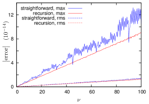
Figure 1: Maximum and root-mean-square errors in the values of $\cos\nu\theta$ and $\sin\nu\theta$, numerically calculated with 64-bit floating-point numbers, over $0\leq\theta\leq\pi$. The values of $\theta$ are sampled with a uniform spacing of $10^{-5}$ degree. The abscissa is $\nu=0,\frac{1}{2},1,\cdots,100$. Recursion means the usage of Eq. (30) together with the initial values described in the following sentences.

Straightforward evaluation of $\cos\,\nu\theta$ and $\sin\,\nu\theta$ (i.e., passing the value of $\nu\theta$ to the internal functions cos and sin) requires about $j$ calls to the functions and is computationally very inefficient. Moreover, as shown in Fig. 1, such straightforward evaluation causes slightly larger numerical errors probably due to the loss of significant digits in reducing the value of $\nu\theta$ to an interval such as $[-\frac{\pi}{4},\frac{\pi}{4}]$, especially when the value of $|\nu\theta|$ is large. The reason why the recursion formula (30) does not suffer from large errors even after hundred steps may be attributed to the fact that the magnitudes of cos and sin functions are always not greater than one.

IV Precision of the numerical values of the $d$ function

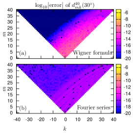
Figure 2: The common logarithm of the error in the 64-bit floating-point numerical value of the $d$ function $d^{j}_{mk}(\theta)$ as a function of $m$ and $k$ for $j=40$ and $\theta=30^{\circ}$. The value of the $d$ function is calculated by means of the Wigner formula in part (a) and the Fourier series expression in part (b). Only a quarter of the possible combinations of $m$ and $k$ are plotted because the error is symmetric in the lines $m=\pm k$. Errors smaller than $10^{-20}$ are painted with the same color as that for the error of $10^{-20}$.

In this section, I compare the errors of the values of $d^{j}_{mk}(\theta)$ calculated with 64-bit floating-point numbers according to the Wigner formula (3) and the Fourier series expression (10). The errors have been calculated as the differences from the exact values calculated by applying a formula-manipulation software MAXIMA to the Wigner formula.

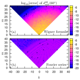
Figure 3: The same as in Fig. 2 but for $\theta=60^{\circ}$.

Figures 2,  3, and 4 show the errors for $\theta=30^{\circ}$, $60^{\circ}$, and $90^{\circ}$, respectively. The errors are expressed as a function of $(m,k)$ while $j$ is fixed at 40. I have found that similar plots for $\theta>90^{\circ}$ look almost indistinguishable from those for $180^{\circ}-\theta$ except that the sign of $k$ is reversed, as could be foreseen from Eq. (39).

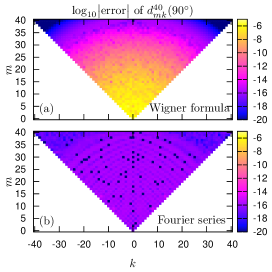
Figure 4: The same as in Fig. 2 but for $\theta=90^{\circ}$.

One can see that the Wigner formula results in very large errors, up to $\sim 10^{-5}$ for $\theta\sim 90^{\circ}$ and $m\sim k\sim 0$, while the Fourier series expression gives precisely 15 digits irrespective of the values of $\theta$, $j$, $m$, and $k$. I confidently recommend the Fourier series expression over the Winger formula already at $j\sim 40$.

For a special purpose, however, the Wigner formula still has an advantage. For regions of the arguments $\theta\sim 0^{\circ}$ ($180^{\circ}$) and $|m+k|\sim 0$ ($2j$), the Wigner formula has smaller errors than $10^{-15}$, i.e., than the level of the almost constant error of the Fourier series expression. In such regions of the arguments, the magnitude of $d^{j}_{mk}(\theta)$ is very small and a small number of terms dominate in the summation of the Wigner formula, while many terms of order 1 cancel among themselves to give the small value in the Fourier series expression. Therefore, if one needs such high precision at those regions, it would be a good idea to develop a program which switches between the two formulas depending on the values of $\theta$, $j$, $m$, and, $k$.

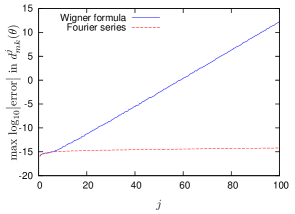
Figure 5: The common logarithm of the maximum error in the numerical value of the $d$ function $d^{j}_{mk}(\theta)$ versus $j$ calculated with the Wigner formula (blue solid line) and the Fourier series expression (red dashed line). The maximum is taken over the values of $m$, $k$, and $\theta$ for each $j$.

In Fig. 5, I compare the maximum errors of $d^{j}_{mk}(\theta)$ as functions of $j$. The maximum is taken over the values of $\theta$ from $0^{\circ}$ to $180^{\circ}$ with an increment of $5^{\circ}$ and all possible combinations of $m$ and $k$. For both formulas, the maximum error increases as exponential functions of $j$. The Wigner formula increases its error, however, far faster than the Fourier series expression. For the interval $20\leq j\leq 100$, the error of the Wigner formula can be approximated by $\log_{10}|{\rm error}|\approx 0.294j-17.2$ while that of the Fourier series expression can be approximated by $\log_{10}|{\rm error}|\approx 0.006j-14.8$. In other words, by increasing $j$ by one, the error of the Wigner formula is doubled, while that of the Fourier series expression increases only by 1.4%.

V Summary

I have shown that the Wigner formula for the $d$ function results in intolerable large numerical errors for large values of the angular momentum quantum number $j$. On the other hand, the Fourier series expression for the $d$ function is shown to be free of such errors, providing precision of $\sim 10^{-14}$ even at $j=100$. An analytic expression for the coefficients of the Fourier series is given. Their numerical values, which are precise as far as 64-bit floating-point numbers can express, are provided as electric files in Supplemental Material. Sample programs in FORTRAN90 to use the data files are also provided.

Appendix A Properties of the $d$ function utilized in this paper

I enumerate the symmetries of the $d$ function to be referred to in this paper.

First, the unitarity of rotations (i.e, the Hermite conjugate operator is the inverse operator) means

$$d^{j}_{mk}(\theta)=d^{j}_{km}(-\theta).$$ (31)

Second, the composition of two rotations can be rewritten as multiplication of matrices to represent them,

$$d^{j}_{mk}(\theta_{1}+\theta_{2})=\sum_{\nu=-j}^{j}d^{j}_{m\nu}(\theta_{1})d^{j}_{\nu k}(\theta_{2}).$$ (32)

I need three more relations, whose easiest derivation may be to use the Wigner formula (3) as in Ref. Rose (1957),

$$d^{j}_{mk}(\theta) = (-1)^{m-k}d^{j}_{mk}(-\theta),$$ (33)

$$d^{j}_{mk}(\theta) = d^{j}_{-k,-m}(\theta),$$ (34)

$$d^{j}_{mk}(\pi) = (-1)^{j+m}\delta_{m,-k}.$$ (35)

From Eqs. (31) and (33), one can prove

$$d^{j}_{mk}(\theta)=(-1)^{m-k}d^{j}_{km}(\theta),$$ (36)

from Eqs. (34) and (36),

$$d^{j}_{mk}(\theta)=(-1)^{m-k}d^{j}_{-m,-k}(\theta),$$ (37)

and from Eqs. (32), (35), and (36),

$$d^{j}_{mk}(\pi+\theta)=(-1)^{j+m}d^{j}_{-m,k}(\theta),$$ (38)

$$d^{j}_{mk}(\pi-\theta)=(-1)^{j+m}d^{j}_{m,-k}(\theta).$$ (39)

References

- Rose (1957) M. Rose, Elementary Theory of Angular Momentum (John Wiley and Sons, New York, 1957).
- Bohr and Mottelson (1969) A. Bohr and B. Mottelson, Nuclear Structure vol. I (Benjamin, New York, 1969).
- Tajima (2013) N. Tajima, Journal of Physics: Conference Series 445, 012014 (2013).
- Tajima and Otsuka (2011) N. Tajima and T. Otsuka, Phys. Rev. C 84, 064316 (2011).
- Choi et al. (1999) C. Choi, J. Ivanic, M. Gordon, and K. Ruedenberg, J. Chem. Phys. 111, 8825 (1999).
- Dachsel (2006) H. Dachsel, J. Chem. Phys. 124, 144115 (2006).
-
(7)
See Supplemental Material at http://link.aps.org/
supplemental/10.1103/PhysRevC.91.014320 for the numerical values of the coefficients of the Fourier series of the functions and sample programs to use the data.