On the four-zero texture of quark mass matrices and its stability

Abstract

We carry out a new study of quark mass matrices $M_{\rm u}$ (up-type) and $M_{\rm d}$ (down-type) which are Hermitian and have four zero entries, and find a new part of the parameter space which was missed in the previous works. We identify two more specific four-zero patterns of $M_{\rm u}$ and $M_{\rm d}$ with fewer free parameters, and present two toy flavor-symmetry models which can help realize such special and interesting quark flavor structures. We also show that the texture zeros of $M_{\rm u}$ and $M_{\rm d}$ are essentially stable against the evolution of energy scales in an analytical way by using the one-loop renormalization-group equations.

I Introduction

The discovery of the Higgs boson H signifies the “completion” of the Standard Model (SM) which is not only phenomenologically successful but also theoretically self-consistent. In particular, it verifies the Brout-Englert-Higgs mechanism and Yukawa interactions which are responsible for the generation of lepton and quark masses. However, the SM is not really “complete” in the sense that it cannot explain the origin of neutrino masses, the structures of lepton and quark flavors, the asymmetry of matter and antimatter in the Universe, the nature of dark matter, etc. Hence one has to go beyond the SM and explore possible new physics behind it in order to solve the aforementioned puzzles.

Here let us focus on the flavor puzzles in the SM. The flavor issues mainly refer to the generation of fermion masses, the dynamics of flavor mixing and the origin of CP violation. Even within the SM in which all the neutrinos are assumed to be massless, there are thirteen free flavor parameters which have to be experimentally determined. On the other hand, one is also puzzled by the observed spectra of lepton and quark masses and the observed patterns of flavor mixing, which must imply a kind of underlying flavor structure Xing2014 .

In this paper we restrict ourselves to the flavor issues in the quark sector where there are ten free parameters: six quark masses, three flavor mixing angles and one CP-violating phase. Thanks to the coexistence of Yukawa interactions and charged-current gauge interactions, the flavor and mass bases of three quark families do not coincide with each other, leading to the phenomenon of flavor mixing and CP violation. The latter is described by a $3\times 3$ unitary matrix $V$, the so-called Cabibbo-Kobayashi-Maskawa (CKM) matrix CKM ,

$$V=\left(\begin{matrix}V_{ud}&V_{us}&V_{ub}\cr V_{cd}&V_{cs}&V_{cb}\cr V_{td}&V_{ts}&V_{tb}\cr\end{matrix}\right)\;,$$ (1)

which can be parameterized in terms of three mixing angles ($\theta_{12},\theta_{13},\theta_{23}$) and one CP-violating phase ($\delta$) via the definitions of $V_{us}=\sin\theta_{12}\cos\theta_{13}$, $V_{ub}=\sin\theta_{13}e^{-{\rm i}\delta}$ and $V_{cb}=\cos\theta_{13}\sin\theta_{23}$ and the unitarity of $V$ itself. As $V$ originates from a mismatch between the diagonalizations of the up-type quark mass matrix $M_{\rm u}$ and the down-type one $M_{\rm d}$, which are equivalent to transforming their flavor bases into their mass bases, an attempt to calculate the flavor mixing parameters should start from the mass matrices in the flavor basis. In view of the experimental results $m_{u}\ll m_{c}\ll m_{t}$, $m_{d}\ll m_{s}\ll m_{b}$ and $\theta_{13}\ll\theta_{23}\ll\theta_{12}\equiv\theta_{\rm C}\simeq 13^{\circ}$, where $\theta_{\rm C}$ denotes the Cabibbo angle, we believe that the strong hierarchy of three flavor mixing angles must be attributed to the strong hierarchy of quark masses.

Therefore, one is tempted to relate the smallness of three flavor mixing angles with the smallness of four independent mass ratios $m_{u}/m_{c}$, $m_{c}/m_{t}$, $m_{d}/m_{s}$ and $m_{s}/m_{b}$. A famous relation of this kind is the Gatto-Sartori-Tonin (GST) relation $\sin\theta_{12}\sim\sqrt{m_{d}/m_{s}}$ gst . The Fritzsch ansatz of quark mass matrices fritzsch ,

$$M^{\rm F}_{{\rm u}}=\left(\begin{array}[]{ccc}0&C_{{\rm u}}&0\\ C_{{\rm u}}^{*}&0&B_{{\rm u}}\\ 0&B_{{\rm u}}^{*}&A_{{\rm u}}\end{array}\right)\;,\hskip 42.67912ptM^{\rm F}_{{\rm d}}=\left(\begin{array}[]{ccc}0&C_{{\rm d}}&0\\ C_{{\rm d}}^{*}&0&B_{{\rm d}}\\ 0&B_{{\rm d}}^{*}&A_{{\rm d}}\end{array}\right)\;,$$ (2)

can easily lead us to the above GST relation. Note that $M^{\rm F}_{{\rm u}}$ and $M^{\rm F}_{{\rm d}}$ possess the parallel structures with the same zero entries. Furthermore, they have been taken to be Hermitian without loss of generality, since a rotation of the right-handed quark fields does not affect any physical results in the SM or its extensions which have no flavor-changing right-handed currents. The Fritzsch ansatz totally involves eight independent parameters, and thus it can predict two relations among six quark masses and four flavor mixing parameters. However, it has been shown that this simple ansatz is in conflict with current experimental data sixzero .

One may modify the Fritzsch ansatz by reducing the number of its texture zeros. Given a Hermitian or symmetric mass matrix, a pair of its off-diagonal texture zeros are always counted as one zero. Hence the Fritzsch ansatz has six nontrivial texture zeros. It has been shown that adding nonzero (1,1) or (1,3) entries to $M^{\rm F}_{\rm u}$ and $M^{\rm F}_{\rm d}$ does not help much Shrock , but the following Fritzsch-like ansatz is phenomenologically viable fourzero ; fourzero2 :

$$M_{{\rm u}}=\left(\begin{array}[]{ccc}0&C_{{\rm u}}&0\\ C_{{\rm u}}^{*}&\tilde{B}_{{\rm u}}&B_{{\rm u}}\\ 0&B_{{\rm u}}^{*}&A_{{\rm u}}\end{array}\right)\;,\hskip 42.67912ptM_{{\rm d}}=\left(\begin{array}[]{ccc}0&C_{{\rm d}}&0\\ C_{{\rm d}}^{*}&\tilde{B}_{{\rm d}}&B_{{\rm d}}\\ 0&B_{{\rm d}}^{*}&A_{{\rm d}}\end{array}\right)\;.$$ (3)

We see that Hermitian $M_{{\rm u}}$ and $M_{{\rm d}}$ have the up-down parallelism and four texture zeros. So far a lot of interest has been paid to the phenomenological consequences of Eq. (3) fourzero ; fourzero2 ; previous ; recent . In particular, the parameter space of this ansatz was numerically explored in Ref. xingzhang , where a mild hierarchy $|B|/A\sim\tilde{B}/|B|\sim 0.24$ was found to be favored for both up and down sectors. Here we have omitted the subscript “u” and “d” for the relevant parameters, and we shall do so again when discussing something common to $M_{{\rm u}}$ and $M_{{\rm d}}$ throughout this paper. Although there are four complex parameters in Eq. (3), only two linear combinations of the four phases are physical and can simply be denoted as $\phi_{1}=\arg(C_{\rm u})-\arg(C_{\rm d})$ and $\phi_{2}=\arg(B_{\rm u})-\arg(B_{\rm d})$. It has been found that $\phi_{2}$ is very close to zero or $2\pi$ xingzhang , while $\sin{\phi_{1}}$ is close to $\pm 1$ and its sign can be fixed by $\eta_{\rm u}\eta_{\rm d}\sin{\phi_{1}}>0$, where the dimensionless coefficients $\eta_{\rm u}$ and $\eta_{\rm d}$ will be defined in section II.

In this paper we aim to carry out a new study of the four-zero texture of quark mass matrices and improve the previous works in the following aspects:

• We reexplore the parameter space of $M_{\rm u}$ and $M_{\rm d}$ by taking into account the updated values of quark masses and the latest results of the CKM flavor mixing parameters. The new analysis leads us to a new part of the parameter space, which is interesting but was missed in Ref. xingzhang and other references.

• We identify two more specific four-zero patterns of $M_{\rm u}$ and $M_{\rm d}$ with fewer free parameters. Namely, there is a kind of parameter correlation in such an ansatz, making the exercise of model building much easier. We present two toy flavor-symmetry models to realize such special and interesting quark flavor structures.

• The running behaviors of $M_{\rm u}$ and $M_{\rm d}$ from a superhigh scale down to the electroweak scale are studied in an analytical way by using the one-loop renormalization-group equations (RGEs), in order to examine whether those texture zeros are stable against the evolution of energy scales. We find that they are essentially stable in the SM.

The remaining parts of this paper are organized as follows. In section II we first explore the complete parameter space of $M_{\rm u}$ and $M_{\rm d}$ and then discuss the relevant phenomenological consequences. Particular attention will be paid to some properties of the four-zero texture that the previous works did not put emphasis on. Section III is devoted to discussions about the special patterns of four-zero quark mass matrices in which some particular relations among the finite matrix elements are possible. Two toy flavor-symmetry models, which can help realize such interesting patterns, will be presented for the sake of illustration. In section IV we derive the one-loop RGE corrections to $M_{\rm u}$ and $M_{\rm d}$ which evolve from a superhigh energy scale down to the electroweak scale. Our analytical results show that those texture zeros are essentially stable against the evolution of energy scales. As a byproduct, the possibility of applying the four-zero texture of quark mass matrices to resolving the strong CP problem is also discussed in a brief way. Finally, we summarize our main results and make some concluding remarks on the quark flavor issues in section V.

II The parameter space: results and explanations

Before performing an updated and complete numerical analysis of the parameter space of Hermitian $M_{\rm u}$ and $M_{\rm d}$ with four texture zeros, let us briefly reformulate the relations between the parameters of $M_{\rm u,d}$ and the observable quantities xingzhang . First of all, $M_{\rm u,d}$ can be transformed into a real symmetric matrix $\overline{M}_{\rm u,d}$ through a phase redefinition:

$$\overline{M}=P^{\dagger}MP=\left(\begin{array}[]{ccc}0&\hskip 8.5359pt|C|&\hskip 8.5359pt0\\ |C|&\hskip 8.5359pt\tilde{B}&\hskip 8.5359pt|B|\\ 0&\hskip 8.5359pt|B|&\hskip 8.5359ptA\end{array}\right)\;,$$ (4)

where the subscript “u” or “d” has been omitted, and $P={\rm Diag}\{1,e^{-{\rm i}\phi_{C}},e^{-{\rm i}(\phi_{C}+\phi_{B})}\}$ with $\phi_{B}=\arg(B)$ and $\phi_{C}=\arg(C)$. Of course, one may diagonalize $\overline{M}$ as follows:

$$O^{\rm T}\overline{M}O=\left(\begin{array}[]{ccc}\lambda_{1}&&\\ &\hskip 8.5359pt\lambda_{2}&\\ &&\hskip 8.5359pt\lambda_{3}\end{array}\right)\;.$$ (5)

Without loss of generality, we require $A$ and $\lambda_{3}$ to be positive. Then $|B|$, $\tilde{B}$ and $|C|$ can be expressed in terms of $A$ and the three quark mass eigenvalues $\lambda_{i}$ (for $i=1,2,3$, corresponding to $m_{u},m_{c},m_{t}$ in the up sector or $m_{d},m_{s},m_{b}$ in the down sector):

$$\begin{array}[]{cll}\vspace{0.2cm}\tilde{B}&=&\lambda_{1}+\lambda_{2}+\lambda_{3}-A\ ,\\ \vspace{0.2cm}|B|&=&\sqrt{\displaystyle\frac{\left(A-\lambda_{1}\right)\left(A-\lambda_{2}\right)\left(\lambda_{3}-A\right)}{A}}\ ,\\ |C|&=&\sqrt{\displaystyle\frac{-\lambda_{1}\lambda_{2}\lambda_{3}}{A}}\ .\end{array}$$ (6)

In this case the orthogonal matrix $O$ reads

$$O=\left(\begin{array}[]{ccc}\vspace{0.3cm}\sqrt{\displaystyle\frac{\lambda_{2}\lambda_{3}\left(A-\lambda_{1}\right)}{A\left(\lambda_{2}-\lambda_{1}\right)\left(\lambda_{3}-\lambda_{1}\right)}}&\hskip 14.22636pt\displaystyle\eta\sqrt{\frac{\lambda_{1}\lambda_{3}\left(\lambda_{2}-A\right)}{A\left(\lambda_{2}-\lambda_{1}\right)\left(\lambda_{3}-\lambda_{2}\right)}}&\hskip 14.22636pt\displaystyle\sqrt{\frac{\lambda_{1}\lambda_{2}\left(A-\lambda_{3}\right)}{A\left(\lambda_{3}-\lambda_{1}\right)\left(\lambda_{3}-\lambda_{2}\right)}}\\ \vspace{0.3cm}\displaystyle-\eta\sqrt{\frac{\lambda_{1}\left(\lambda_{1}-A\right)}{\left(\lambda_{2}-\lambda_{1}\right)\left(\lambda_{3}-\lambda_{1}\right)}}&\hskip 14.22636pt\displaystyle\sqrt{\frac{\lambda_{2}\left(A-\lambda_{2}\right)}{\left(\lambda_{2}-\lambda_{1}\right)\left(\lambda_{3}-\lambda_{2}\right)}}&\hskip 14.22636pt\displaystyle\sqrt{\frac{\lambda_{3}\left(\lambda_{3}-A\right)}{\left(\lambda_{3}-\lambda_{1}\right)\left(\lambda_{3}-\lambda_{2}\right)}}\\ \vspace{0.3cm}\displaystyle\eta\sqrt{\frac{\lambda_{1}\left(A-\lambda_{2}\right)\left(A-\lambda_{3}\right)}{A\left(\lambda_{2}-\lambda_{1}\right)\left(\lambda_{3}-\lambda_{1}\right)}}&\displaystyle-\sqrt{\frac{\lambda_{2}\left(A-\lambda_{1}\right)\left(\lambda_{3}-A\right)}{A\left(\lambda_{2}-\lambda_{1}\right)\left(\lambda_{3}-\lambda_{2}\right)}}&\displaystyle\sqrt{\frac{\lambda_{3}\left(A-\lambda_{1}\right)\left(A-\lambda_{2}\right)}{A\displaystyle\left(\lambda_{3}-\lambda_{1}\right)\left(\lambda_{3}-\lambda_{2}\right)}}\end{array}\right)\;,$$ (7)

where $\eta=\pm 1$, and the emergence of this coefficient can be understood as follows. Since $A$ and $\lambda_{3}$ have been taken to be positive, $\lambda_{1}$ and $\lambda_{2}$ must have the opposite signs so as to assure a negative value of the determinant of $\overline{M}$,

$${\rm Det}(\overline{M})=-A|C|^{2}=\lambda_{1}\lambda_{2}\lambda_{3}\ .$$ (8)

When identifying $\lambda_{1,2,3}$ with the physical quark masses, we use $\eta=+1$ and $-1$ to label the cases $(\lambda_{1},\lambda_{2},\lambda_{3})=(-m_{u},m_{c},m_{t})$ and $(\lambda_{1},\lambda_{2},\lambda_{3})=(m_{u},-m_{c},m_{t})$ in the up sector, respectively. The same labeling is valid for the down sector.

In terms of quark mass eigenstates, the weak charged-current interactions are written as

$$-{\cal L}_{\rm cc}=\frac{g_{2}}{\sqrt{2}}~{}\overline{\left(u~{}~{}c~{}~{}t\right)_{\rm L}}~{}\gamma^{\mu}\ V\left(\begin{matrix}d\cr s\cr b\cr\end{matrix}\right)_{\rm L}W^{+}_{\mu}+{\rm h.c.}\;,$$ (9)

where the CKM matrix $V$ appears in the form $V=O_{\rm u}^{\rm T}P_{\rm u}^{*}P_{\rm d}O_{\rm d}$. The nine elements of $V$ can be explicitly expressed as

$$V_{i\alpha}=O_{1i}^{\rm u}O_{1\alpha}^{\rm d}+O_{2i}^{\rm u}O_{2\alpha}^{\rm d}e^{{\rm i}\phi_{1}}+O_{3i}^{\rm u}O_{3\alpha}^{\rm d}e^{{\rm i}\left(\phi_{1}+\phi_{2}\right)}\ ,$$ (10)

where $\phi_{1}=\phi_{C_{\rm u}}-\phi_{C_{\rm d}}$ and $\phi_{2}=\phi_{B_{\rm u}}-\phi_{B_{\rm d}}$, and the subscripts $i$ and $\alpha$ run over $(u,c,t)$ and $(d,s,b)$, respectively. Now it is clear that $V$ depends on four free parameters $A_{\rm u}$, $A_{\rm d}$, $\phi_{1}$ and $\phi_{2}$, after the quark masses are input. With the help of the above analytical results, we are able to constrain the parameter space of $M_{\rm u}$ and $M_{\rm d}$ by taking account of the latest values of the CKM matrix elements pdg

$$|V|=\left(\begin{array}[]{ccc}0.97427\pm 0.00014&\hskip 28.45274pt0.22536\pm 0.00061&\hskip 28.45274pt0.00355\pm{0.00015}\\ 0.22522\pm 0.00061&\hskip 28.45274pt0.97343\pm 0.00015&\hskip 28.45274pt0.0414\pm{0.0012}\\ 0.00886\pm{0.00033}&\hskip 28.45274pt0.0405\pm{0.0012}&\hskip 28.45274pt0.99914\pm{0.00005}\end{array}\right)\;,$$ (11)

together with the updated values of quark masses at the scale of $M_{Z}$ mass

$$\begin{array}[]{lll}m_{u}=1.38^{+0.42}_{-0.41}\ {\rm MeV}\ ,&\hskip 28.45274ptm_{c}=638^{+43}_{-84}\ {\rm MeV}\ ,&\hskip 28.45274ptm_{t}=172.1\pm 1.2\ {\rm GeV}\ ,\\ m_{d}=2.82\pm 0.48\ {\rm MeV}\ ,&\hskip 28.45274ptm_{s}=57^{+18}_{-12}\ {\rm MeV}\ ,&\hskip 28.45274ptm_{b}=2860^{+160}_{-60}\ {\rm MeV}\ .\end{array}$$ (12)

In our numerical analysis, we prefer to use $|V_{us}|$, $|V_{ub}|$, $|V_{cb}|$ and the CP-violating observable $\sin 2\beta$ as the inputs because their values have been determined to a very good degree of accuracy. Here $\beta$ stands for one of the inner angles of the CKM unitarity triangle described by the orthogonality relation $V_{ub}^{*}V_{ud}+V_{cb}^{*}V_{cd}+V_{tb}^{*}V_{td}=0$ in the complex plane. The three inner angles of this triangle are defined as

$$\alpha=\arg\left(-\displaystyle\frac{V_{tb}^{*}V_{td}}{V_{ub}^{*}V_{ud}}\right)\ ,\hskip 28.45274pt\beta=\arg\left(-\displaystyle\frac{V_{cb}^{*}V_{cd}}{V_{tb}^{*}V_{td}}\right)\ ,\hskip 28.45274pt\gamma=\arg\left(-\displaystyle\frac{V_{ub}^{*}V_{ud}}{V_{cb}^{*}V_{cd}}\right)\ ,$$ (13)

and their experimental values are pdg

$$\alpha=\left(85.4^{+3.9}_{-3.8}\right)^{\circ}\ ,\hskip 28.45274pt\sin{2\beta}=0.682\pm 0.019\ ,\hskip 28.45274pt\gamma=\left(68.0^{+8.0}_{-8.5}\right)^{\circ}\ .$$ (14)

Obviously, the uncertainty associated with $\sin 2\beta$ is much smaller than those associated with $\alpha$ and $\gamma$. The unitarity of $V$ requires $\alpha+\beta+\gamma=\pi$.

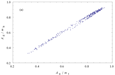
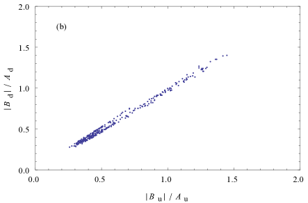
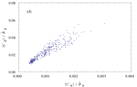
Figure 1: The allowed regions of $A_{\rm u,d}$, $|B_{\rm u,d}|$, $\tilde{B}_{\rm u,d}$ and $|C_{\rm u,d}|$ as constrained by current experimental data in the $(\eta_{\rm u},\eta_{\rm d})=(+1,+1)$ case.

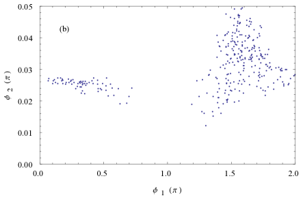
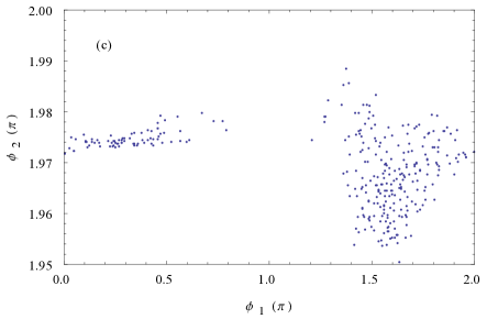
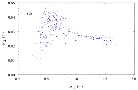
Figure 2: The allowed regions of $\phi_{1}$ and $\phi_{2}$ as constrained by current experimental data in the $(\eta_{\rm u},\eta_{\rm d})=(\pm 1,\pm 1)$ cases.

FIG. 1(a) shows the allowed region of $A_{\rm u}$ and $A_{\rm d}$, which are rescaled as $r_{\rm u}=A_{\rm u}/m_{t}$ and $r_{\rm d}=A_{\rm d}/m_{b}$, in the $(\eta_{\rm u},\eta_{\rm d})=(+1,+1)$ case. Since the results of $r_{\rm u}$ and $r_{\rm d}$ in the other three cases are not quite different from that illustrated in FIG. 1(a), here we just concentrate on the $(\eta_{\rm u},\eta_{\rm d})=(+1,+1)$ case for the sake of simplicity. Now that $r_{\rm u}\simeq r_{\rm d}$ is a quite good approximation as shown in FIG. 1(a), we simply use $r$ to denote both $r_{\rm u}$ and $r_{\rm d}$ when their difference needs not to be mentioned. We find that the region of $r$ can be roughly divided into two parts: (1) $r$ is close to 1 and mainly lies in the range of $0.8$ to $0.9$; (2) $r$ is around 0.5 and mainly ranges from $0.4$ to $0.6$. These two parts will be referred to as the $r\sim 1$ and $r\sim 0.5$ regions, respectively, in the following discussions. The reasonableness of this treatment will become clear shortly, since the phase parameters $\phi_{1}$ and $\phi_{2}$ behave very differently in these two regions.

The allowed regions of $\phi_{1}$ and $\phi_{2}$ are shown in FIG. 2, where the possibilities of $(\eta_{\rm u},\eta_{\rm d})=(+1,+1),(+1,-1),(-1,+1)$ and $(-1,-1)$ have all been considered. Taking the $(+1,+1)$ case for example, we find that $\phi_{2}$ is very close to 2$\pi$ and thus its allowed range can also be denoted as $\phi_{2}\lesssim 0$. In comparison, the allowed range of $\phi_{1}$ is much wider but it can also be divided into two parts in a reasonable approximation: $\phi_{1}\sim 0.5\pi$ and $\phi_{1}\sim 1.5\pi$. There is actually a correlation between $r$ and $\phi_{1}$: in the $r\sim 1$ region $\phi_{1}\sim 0.5\pi$ holds, and in the $r\sim 0.5$ region $\phi_{1}\sim 1.5\pi$ holds. After examining all the four $(\eta_{\rm u},\eta_{\rm d})=(\pm 1,\pm 1)$ cases, we obtain the more general correlation between $r$ and $\phi_{1,2}$ as follows:

$$\begin{array}[]{ll}\eta_{\rm u}\ \eta_{\rm d}\ \sin{\phi_{1}}>0\hskip 5.69046pt{\rm for}\hskip 5.69046ptr\sim 1\ ;&\hskip 19.91684pt\eta_{\rm u}\ \eta_{\rm d}\ \sin{\phi_{1}}<0\hskip 5.69046pt{\rm for}\hskip 5.69046ptr\sim 0.5\ ;\\ \eta_{\rm d}\ \sin{\phi_{2}}<0\ ;&\hskip 19.91684pt\eta_{\rm u}\ \eta_{\rm d}\ \cos{\phi_{1}}<0\ .\\ \end{array}$$ (15)

Note that only the constraint $\eta_{\rm d}\sin{\phi_{2}}<0$ is numerically exact, and the other three constraints serve for good approximations in which most scattered points are satisfied. Such correlative constraints can also be given in a more explicit way, as listed in TABLE i@. Finally let us point out that the $r\sim 1$ region and its corresponding parameter correlation found here are consistent with the results presented in Ref. xingzhang , but the $r\sim 0.5$ region and its parameter correlation are our new findings which were missed in the previous works (mainly because $\phi_{1}$ takes totally different values in this region from our expectation based on its values in the $r\sim 1$ region).

Table 1: The correlation between $r$ and $\phi_{1,2}$ in the four $(\eta_{\rm u},\eta_{\rm d})=(\pm 1,\pm 1)$ cases.

	$r\sim 1$	$r\sim 0.5$
$(\eta_{\rm u},\eta_{\rm d})=(+1,+1)$	$\phi_{1}\sim 0.5\pi$ ,   $\cos{\phi_{1}}<0$ ,   $\phi_{2}\lesssim 0$ .	$\phi_{1}\sim 1.5\pi$ ,  $\cos{\phi_{1}}<0$ ,  $\phi_{2}\lesssim 0$ .
$(\eta_{\rm u},\eta_{\rm d})=(+1,-1)$	$\phi_{1}\sim 1.5\pi$ ,   $\cos{\phi_{1}}>0$ ,  $\phi_{2}\gtrsim 0$ .	$\phi_{1}\sim 0.5\pi$ ,  $\cos{\phi_{1}}>0$ ,  $\phi_{2}\gtrsim 0$ .
$(\eta_{\rm u},\eta_{\rm d})=(-1,+1)$	$\phi_{1}\sim 1.5\pi$ ,   $\cos{\phi_{1}}>0$ ,  $\phi_{2}\lesssim 0$ .	$\phi_{1}\sim 0.5\pi$ ,  $\cos{\phi_{1}}>0$ ,  $\phi_{2}\lesssim 0$ .
$(\eta_{\rm u},\eta_{\rm d})=(-1,-1)$	$\phi_{1}\sim 0.5\pi$ ,   $\cos{\phi_{1}}<0$ ,  $\phi_{2}\gtrsim 0$ .	$\phi_{1}\sim 1.5\pi$ ,  $\cos{\phi_{1}}<0$ ,   $\phi_{2}\gtrsim 0$ .

All the correlative constraints listed in TABLE I can find an explanation once the analytical expression of the CKM matrix $V$ is explicitly presented. No matter whether the region $r\sim 1$ or $r\sim 0.5$ is concerned, one can easily check that $A$ is close to the mass of the third-family quark and thus it is much larger than the masses of the first- and second-family quarks. As a result, the orthogonal matrices $O_{\rm u}$ and $O_{\rm d}$ can approximate to

$$O_{\rm u} \simeq \left(\begin{array}[]{ccc}\vspace{0.3cm}1&\hskip 14.22636pt\eta_{\rm u}\sqrt{\displaystyle\frac{m_{u}}{m_{c}}}&\hskip 14.22636pt0\\ \vspace{0.3cm}-\eta_{\rm u}\sqrt{\displaystyle r_{\rm u}\ \frac{m_{u}}{m_{c}}}&\hskip 14.22636pt\sqrt{r_{\rm u}}&\hskip 14.22636pt\sqrt{1-r_{\rm u}}\\ \vspace{0.3cm}\eta_{\rm u}\sqrt{(1-r_{\rm u})\ \displaystyle\frac{m_{u}}{m_{c}}}&\hskip 14.22636pt-\sqrt{1-r_{\rm u}}&\hskip 14.22636pt\sqrt{r_{\rm u}}\\ \end{array}\right)\;,$$ (19)

$$O_{\rm d} \simeq \left(\begin{array}[]{ccc}\vspace{0.3cm}1&\hskip 14.22636pt\eta_{\rm d}\sqrt{\displaystyle\frac{m_{d}}{m_{s}}}&\hskip 14.22636pt\sqrt{\left(\displaystyle\frac{1}{r_{\rm d}}-1\right)\displaystyle\frac{m_{d}}{m_{b}}\ \frac{m_{s}}{m_{b}}}\\ \vspace{0.3cm}-\eta_{\rm d}\sqrt{r_{\rm d}\ \displaystyle\frac{m_{d}}{m_{s}}}&\hskip 14.22636pt\sqrt{r_{\rm d}}&\hskip 14.22636pt\sqrt{1-r_{\rm d}}\\ \vspace{0.3cm}\eta_{\rm d}\sqrt{(1-r_{\rm d})\left(1-\ \displaystyle\frac{\eta_{\rm d}}{r_{\rm d}}\ \displaystyle\frac{m_{s}}{m_{b}}\right)\displaystyle\frac{m_{d}}{m_{s}}}&\hskip 14.22636pt-\sqrt{1-r_{\rm d}}&\hskip 14.22636pt\sqrt{r_{\rm d}\ \left(1-\ \displaystyle\frac{\eta_{\rm d}}{r_{\rm d}}\ \displaystyle\frac{m_{s}}{m_{b}}\right)}\\ \end{array}\right)\;.\hskip 19.91684pt$$ (23)

Because $m_{u}/m_{c}\sim m_{c}/m_{t}\sim\sin^{4}\theta_{\rm C}$ and $m_{d}/m_{s}\sim m_{s}/m_{b}\sim\sin^{2}\theta_{\rm C}$ hold, the (1,3) entry of $O_{\rm u}$ is negligibly small but that of $O_{\rm d}$ is not. Although the factor $m_{s}/(r_{\rm d}m_{b})$ is actually much smaller than 1, it is kept in the (3,1) and (3,3) entries of $O_{\rm d}$ since it will play a crucial role in explaining the correlation $\eta_{\rm d}\sin{\phi_{2}}<0$.

Given the approximate results of $O_{\rm u}$ and $O_{\rm d}$ in Eq. (16), it is straightforward to calculate all the CKM matrix elements by using Eq. (10). We are particularly interested in

$$\begin{aligned} \vspace{0.5cm}|V_{us}|\simeq&\left|\eta_{\rm u}\ \eta_{\rm d}\sqrt{\displaystyle\frac{m_{d}}{m_{s}}}-\sqrt{\displaystyle\frac{m_{u}}{m_{c}}}\ e^{{\rm i}\phi_{1}}\left(\displaystyle\sqrt{r_{\rm u}\ r_{\rm d}}+\sqrt{\displaystyle(1-r_{\rm u})\ (1-r_{\rm d})}\ e^{{\rm i}\phi_{2}}\right)\right|\;,\\ \vspace{0.5cm}|V_{cb}|\simeq&\left|\sqrt{\displaystyle r_{\rm u}\ (1-r_{\rm d})}-\sqrt{\displaystyle(1-r_{\rm u})\ r_{\rm d}\left(1-\ \displaystyle\frac{\eta_{\rm d}}{r_{\rm d}}\ \displaystyle\frac{m_{s}}{m_{b}}\right)}\ e^{{\rm i}\phi_{2}}\right|\;,\\ \vspace{0.5cm}{|V_{ub}|}\simeq&\left|\sqrt{\displaystyle\frac{m_{d}}{m_{b}}\ \frac{m_{s}}{m_{b}}\left(\displaystyle\frac{1}{r_{\rm d}}-1\right)}-\eta_{\rm u}\sqrt{\displaystyle\frac{m_{u}}{m_{c}}}\ V_{cb}\right|\;.\\ \end{aligned}$$ (24)

Among them $|V_{cb}|$ deserves special attention and can be decomposed as follows:

$$\begin{array}[]{ll}\vspace{0.3cm}&|V_{cb}|=\left|\ {\rm Re}\ (V_{cb}^{\prime})-{\rm i}\ {\rm Im}\ (V_{cb}^{\prime})\ \right|=\sqrt{\left[{\rm Re}(V_{cb}^{\prime})\right]^{2}+\left[{\rm Im}(V_{cb}^{\prime})\right]^{2}}\ ,\\ \vspace{0.3cm}&{\rm Re}(V_{cb}^{\prime})\simeq\sqrt{r_{\rm u}\ (1-r_{\rm d})}-\sqrt{(1-r_{\rm u})\ r_{\rm d}\ \left(1-\ \displaystyle\frac{\eta_{\rm d}}{r_{\rm d}}\ \displaystyle\frac{m_{s}}{m_{b}}\right)}\ \cos{\phi_{2}}\ ,\\ &{\rm Im}(V_{cb}^{\prime})\simeq\sqrt{(1-r_{\rm u})\ r_{\rm d}\ \left(1-\ \displaystyle\frac{\eta_{\rm d}}{r_{\rm d}}\ \displaystyle\frac{m_{s}}{m_{b}}\right)}\ \sin{\phi_{2}}\ ,\end{array}$$ (25)

where $V_{cb}^{\prime}=e^{-{\rm i}\phi_{1}}V_{cb}$ has been defined. Clearly, neither $|{\rm Re}\ (V_{cb}^{\prime})|$ nor $|{\rm Im}\ (V_{cb}^{\prime})|$ is allowed to be larger than the experimental result $|V_{cb}|\simeq 0.04$. That is why $r_{\rm u}$ is always nearly equal to $r_{\rm d}$ and $\phi_{2}$ is so close to $0$ or $2\pi$. For either $r_{\rm u}\sim r_{\rm d}\sim 1$ or $r_{\rm u}\sim r_{\rm d}\sim 0.5$, the fact of $\phi_{2}\sim 0$ (or $2\pi$) allows us to simplify the expression of $|V_{us}|$ to

$$\begin{array}[]{l}|V_{us}|\simeq\left|\eta_{\rm u}\ \eta_{\rm d}\sqrt{\displaystyle\frac{m_{d}}{m_{s}}}-\sqrt{\displaystyle\frac{m_{u}}{m_{c}}}\ e^{{\rm i}\phi_{1}}\right|=\sqrt{\displaystyle\frac{m_{d}}{m_{s}}-2\ \eta_{\rm u}\ \eta_{\rm d}\ \sqrt{\displaystyle\frac{m_{u}}{m_{c}}\ \displaystyle\frac{m_{d}}{m_{s}}}\ \cos{\phi_{1}}+\displaystyle\frac{m_{u}}{m_{c}}}\ .\end{array}$$ (26)

It is known that the term $\sqrt{m_{d}/m_{s}}$ itself can fit the experimental value of $|V_{us}|$ to a good degree of accuracy (i.e., the GST relation), and hence one has to control the contribution from the smaller term $\sqrt{m_{u}/m_{c}}$ by adjusting the CP-violating phase $\phi_{1}$. This observation immediately leads to $\cos{\phi_{1}}\sim 0$, or equivalently $\phi_{1}\sim 0.5\pi$ or $1.5\pi$. As first pointed out in Ref. FX95 , the relation in Eq. (19) is essentially compatible with the orthogonality relation $V_{ub}^{*}V_{ud}+V_{cb}^{*}V_{cd}+V_{tb}^{*}V_{td}=0$ after the latter is rescaled by $V^{*}_{cb}$, leading to the striking prediction $\alpha\simeq\phi_{1}\sim 0.5\pi$ for the corresponding CKM unitarity triangle. Needless to say, this prediction is consistent with current experimental data shown in Eq. (14).

In order to understand the correlation between the signs of $\sin\phi_{1,2}$ and those of $\eta_{\rm u,d}$, one needs to consider the impact of the CP-violating observable $\sin 2\beta$ on the parameter space of $M_{\rm u}$ and $M_{\rm d}$. Eqs. (10) and (16) allow us to obtain

$$\begin{array}[]{lll}\vspace{0.2cm}{\rm Re}(V_{cd}V_{cb}^{*})&\simeq&-\eta_{\rm u}\ \displaystyle\sqrt{\frac{m_{u}}{m_{c}}}\ \sin{\phi_{1}}\ {\rm Im}(V_{cb}^{\prime})+\left[\eta_{\rm u}\ \displaystyle\sqrt{\frac{m_{u}}{m_{c}}}\cos{\phi_{1}}-\eta_{\rm d}\ \displaystyle\sqrt{\frac{m_{d}}{m_{s}}}\ \right]{\rm Re}(V_{cb}^{\prime})\ ,\\ \vspace{0.2cm}{\rm Im}(V_{cd}V_{cb}^{*})&\simeq&-\eta_{\rm u}\ \displaystyle\sqrt{\frac{m_{u}}{m_{c}}}\ \sin{\phi_{1}}\ {\rm Re}(V_{cb}^{\prime})-\left[\eta_{\rm u}\ \displaystyle\sqrt{\frac{m_{u}}{m_{c}}}\cos{\phi_{1}}-\eta_{\rm d}\ \displaystyle\sqrt{\frac{m_{d}}{m_{s}}}\ \right]{\rm Im}(V_{cb}^{\prime})\ ,\\ \vspace{0.2cm}{\rm Re}(V_{td}V_{tb}^{*})&\simeq&-\eta_{\rm d}\ \displaystyle\sqrt{\frac{m_{d}}{m_{s}}}\ \left[\displaystyle\frac{\eta_{\rm d}}{r_{\rm d}}\ \displaystyle\frac{m_{s}}{m_{b}}\sqrt{r_{\rm u}\left(1-r_{\rm d}\right)}-{\rm Re}(V_{cb}^{\prime})\right]\ ,\\ {\rm Im}(V_{td}V_{tb}^{*})&\simeq&-\eta_{\rm d}\ \displaystyle\sqrt{\frac{m_{d}}{m_{s}}}\ {\rm Im}(V_{cb}^{\prime})\ .\end{array}$$ (27)

Then the definition of $\beta$ in Eq. (13) leads us to

$$\tan\beta = -\frac{{\rm Re}(V_{cd}V_{cb}^{*})\ {\rm Im}(V_{td}V_{tb}^{*})-{\rm Im}(V_{cd}V_{cb}^{*})\ {\rm Re}(V_{td}V_{tb}^{*})}{{\rm Re}(V_{cd}V_{cb}^{*})\ {\rm Re}(V_{td}V_{tb}^{*})+{\rm Im}(V_{cd}V_{cb}^{*})\ {\rm Im}(V_{td}V_{tb}^{*})}\hskip 14.22636pt$$ (28)

$$\simeq \eta_{\rm u}\ \eta_{\rm d}\ \sin{\phi_{1}}\ \displaystyle\sqrt{\frac{m_{u}}{m_{c}}\ \frac{m_{s}}{m_{d}}}\ -\ \displaystyle\frac{\eta_{\rm d}}{r_{\rm d}}\ \frac{m_{s}}{m_{b}}\ \sqrt{r_{\rm u}\left(1-r_{\rm d}\right)}$$

$$\times\left[1-\eta_{\rm u}\ \eta_{\rm d}\ \cos{\phi_{1}}\sqrt{\displaystyle\frac{m_{u}}{m_{c}}\ \frac{m_{s}}{m_{d}}}\right]\displaystyle\frac{{\rm Im}(V_{cb}^{\prime})}{|V_{cb}|^{2}}\ .$$

Given the experimental value of $\sin 2\beta$ in Eq. (14), we arrive at $\tan\beta=0.394\pm 0.015$. In the $r\sim 1$ region the first term of Eq. (21) is dominant, and thus $\eta_{\rm u}\eta_{\rm d}\sin{\phi_{1}}$ is required to be positive. Note that this term is at most 0.322, if the values of quark masses in Eq. (12) are input. Hence the second term of Eq. (21) has to be positive too. In other words, $\eta_{\rm d}\sin{\phi_{2}}$ should be negative because ${\rm Im}(V_{cb}^{\prime})$ is proportional to $\sin{\phi_{2}}$. Furthermore, $\eta_{\rm u}\eta_{\rm d}\cos{\phi_{1}}$ is likely to be negative to enhance the contribution of the second term of Eq. (21) to $\tan\beta$. When the $r\sim 0.5$ region is concerned, we find that the second term of Eq. (21) becomes important, so $\eta_{\rm d}\sin{\phi_{2}}$ is still required to be negative. Since this term has a chance to saturate the experimental value of $\tan{\beta}$, the first term of Eq. (21) is possible to be negative in such a case. In fact, $\eta_{\rm u}\eta_{\rm d}\sin{\phi_{1}}$ must be negative in the $r\sim 0.5$ region if we take into account the constraint from $|V_{ub}|$. With the help of Eqs. (17) and (18), we have

$${|V_{ub}|}\simeq\left|\sqrt{\displaystyle\frac{m_{d}}{m_{b}}\hskip 2.84544pt\frac{m_{s}}{m_{b}}\left(\displaystyle\frac{1}{r_{\rm d}}-1\right)}+\eta_{\rm u}\ \eta_{\rm d}\ \sin{\phi_{1}}\ \sqrt{\displaystyle\frac{m_{u}}{m_{c}}}\hskip 2.84544pt\left|{\rm Im}(V_{cb}^{\prime})\right|\right|\;.$$ (29)

Taking $r_{\rm d}=0.5$ for example, we find that the first term of Eq. (22) is about 0.0044, larger than the experimental value $|V_{ub}|\simeq 0.0036$. In this case the second term of Eq. (22) should be negative so as to partially offset the contribution from the first term. Therefore, we are left with $\eta_{\rm u}\eta_{\rm d}\sin{\phi_{1}}<0$. However, when the first term is large enough, the second term will fail to offset its extra contribution, bringing about a lower bound about 0.3 for $r_{\rm d}$ as shown in FIG. 1(a).

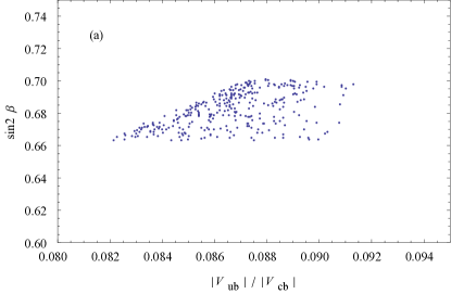
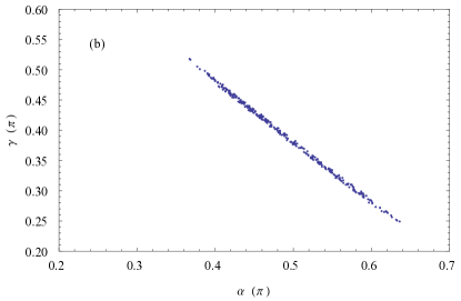
Figure 3: The numerical outputs of $|V_{\rm ub}|/|V_{\rm cb}|$ versus $\sin{2\beta}$ and $\alpha$ versus $\gamma$ in the $(\eta_{\rm u},\eta_{\rm d})=(+1,+1)$ case.

To summarize, we have performed a new numerical analysis of the four-zero ansatz of quark mass matrices by using the updated values of quark masses and CKM parameters. We find a new part of the parameter space of this ansatz — the $r\sim 0.5$ region together with the relevant correlation between $\phi_{1,2}$ and $\eta_{\rm u,d}$. We have also explained the salient features of the whole parameter space of $M_{\rm u}$ and $M_{\rm d}$ in some analytical approximations. As a byproduct, FIG. 3 shows the numerical outputs of $|V_{\rm ub}|/|V_{\rm cb}|$ versus $\sin{2\beta}$ and $\alpha$ versus $\gamma$ in the $(\eta_{\rm u},\eta_{\rm d})=(+1,+1)$ case. One can see that the uncertainties associated with the CP-violating quantities $\alpha$ and $\gamma$ remain quite significant, and they mainly originate from the uncertainties of $m_{s}$, $r_{\rm u}$ and $r_{\rm d}$. In the next section, we shall go back to the quark mass matrices themselves to look at their structures and to see whether they assume some special patterns with fewer free parameters.

III Special four-zero patterns and model building

In the Fritzsch ansatz of quark mass matrices, the first term of Eq. (29) should be replaced with $\left(m_{s}/m_{b}\right)\sqrt{m_{d}/m_{b}}~{}$, whose size is about 0.00078. This result can easily be understood from the trace of $M^{\rm F}_{\rm u,d}$ (i.e., $A=\lambda_{1}+\lambda_{2}+\lambda_{3}$), which gives rise to $r_{\rm d}=1-\mathcal{O}(m_{s}/m_{b})$ in the down sector. Since the upper limit that the second term of Eq. (29) can reach is about 0.00236, the experimental value of $|V_{ub}|$ has no way to be saturated by these two terms in the Fritzsch ansatz. When the four-zero texture of $M_{\rm u,d}$ is concerned, the existence of nonzero (2,2) entries modifies the trace of $M_{\rm u,d}$ to the form $A+\tilde{B}=\lambda_{1}+\lambda_{2}+\lambda_{3}$. The constraint on $r_{\rm d}$ is consequently relaxed, and it actually becomes a free parameter. Given a typical value $r_{\rm d}=0.9$ in the $r\sim 1$ region, for example, the first term of Eq. (29) contributes a value 0.0014 to $|V_{ub}|$ such that the experimental result of $|V_{ub}|$ can be well fitted. In this case the magnitude of $\tilde{B}$ is about 0.1$\lambda_{3}$. To avoid a relatively large $\lambda_{2}$ from such a large $\tilde{B}$, the three parameters $A$, $\tilde{B}$ and $|B|$ must satisfy an approximate geometrical relation fourzero2 up to a correction of $\mathcal{O}(m_{2}/m_{3})$:

$$\frac{|B|}{A}\simeq\displaystyle\frac{\tilde{B}}{|B|}\left[1+\mathcal{O}\left(\displaystyle\frac{m_{2}}{m_{3}}\right)\right]\ .$$ (30)

This observation is certainly supported by the numerical results presented in FIG. 1. In light of the definition $A/m_{3}=r$, $\tilde{B}/m_{3}\simeq 1-r$ holds as a good approximation because of $|\lambda_{1}+\lambda_{2}|\ll\lambda_{3}=m_{3}$. Hence Eq. (30) implies $|B|/m_{3}\simeq\sqrt{r\left(1-r\right)}~{}$. In short, the (2,3) sectors of $\overline{M}_{\rm u}$ and $\overline{M}_{\rm d}$ have the same structure which can be parameterized as

$$\overline{M}_{\rm u}^{(2,3)}\sim A_{\rm u}\left(\begin{array}[]{cc}\epsilon^{2}&\hskip 8.5359pt\epsilon\\ \epsilon&\hskip 8.5359pt1\end{array}\right)\;,\hskip 28.45274pt\overline{M}_{\rm d}^{(2,3)}\sim A_{\rm d}\left(\begin{array}[]{cc}\epsilon^{2}&\hskip 8.5359pt\epsilon\\ \epsilon&\hskip 8.5359pt1\end{array}\right)\;,$$ (31)

where $\epsilon\simeq\sqrt{\left(1-r\right)/r}~{}$, and its value is about 0.3 in the $r\sim 1$ region of the parameter space. Eq. (31) hints at a common origin of the (2,3) sectors of $\overline{M}_{\rm u}$ and $\overline{M}_{\rm d}$, and thus it can be taken as a guideline for model building. However, a numerical analysis shows that such an up-down parallelism is slightly broken by the (2,2) entries of quark mass matrices. In addition, their (1,2) entries do not share this kind of parallelism, as one can see in FIG. 1(d). With the help of Eq. (6), we typically take $r_{\rm u}\simeq r_{\rm d}\simeq 0.9$ and illustrate the finite matrix elements of $\overline{M}_{\rm u}$ and $\overline{M}_{\rm d}$ as follows:

$$\overline{M}_{\rm u}\simeq A_{\rm u}\left(\begin{array}[]{ccc}0&\hskip 5.69046pt0.0002&\hskip 5.69046pt0\\ 0.0002&\hskip 5.69046pt0.11&\hskip 5.69046pt0.31\\ 0&\hskip 5.69046pt0.31&\hskip 5.69046pt1\end{array}\right)\;,\hskip 28.45274pt\overline{M}_{\rm d}\simeq A_{\rm d}\left(\begin{array}[]{ccc}0&\hskip 5.69046pt0.005&\hskip 5.69046pt0\\ 0.005&\hskip 5.69046pt0.13&\hskip 5.69046pt0.31\\ 0&\hskip 5.69046pt0.31&\hskip 5.69046pt1\end{array}\right)\;.$$ (32)

It is worth reiterating that the mild hierarchy in the (2,3) sectors of quark mass matrices is crucial to fit current experimental data.

In the $r\sim 0.5$ region of the parameter space of quark mass matrices $M_{\rm u}$ and $M_{\rm d}$, there is a particularly interesting case,

$$A_{\rm u}=\tilde{B}_{\rm u}\ ,\hskip 28.45274ptA_{\rm d}=\tilde{B}_{\rm d}\ ,$$ (33)

which deserves special attention. We have verified that these exact equalities are really allowed in our numerical calculations. The corresponding parameter space is certainly a part of the parameter space restricted by $r\sim 0.5$. In this special case, the (2,3) sectors of $\overline{M}_{\rm u}$ and $\overline{M}_{\rm d}$ have a neat form:

$$\overline{M}_{\rm u}^{(2,3)}\sim A_{\rm u}\left(\begin{array}[]{cc}\vspace{0.2cm}1&\hskip 5.69046pt1-\displaystyle\frac{2m_{c}}{m_{t}}\\ 1-\displaystyle\frac{2m_{c}}{m_{t}}&\hskip 5.69046pt1\end{array}\right)\;,\hskip 28.45274pt\overline{M}_{\rm d}^{(2,3)}\sim A_{\rm d}\left(\begin{array}[]{cc}\vspace{0.2cm}1&\hskip 5.69046pt1-\displaystyle\frac{2m_{s}}{m_{b}}\\ 1-\displaystyle\frac{2m_{s}}{m_{b}}&\hskip 5.69046pt1\end{array}\right)\;.$$ (34)

A typical numerical illustration of the structures of $\overline{M}_{\rm u}$ and $\overline{M}_{\rm d}$ turns out to be

$$\overline{M}_{\rm u}\simeq A_{\rm u}\left(\begin{array}[]{ccc}0&\hskip 5.69046pt0.0005&\hskip 5.69046pt0\\ 0.0005&\hskip 5.69046pt1&\hskip 5.69046pt0.993\\ 0&\hskip 5.69046pt0.993&\hskip 5.69046pt1\end{array}\right)\;,\hskip 28.45274pt\overline{M}_{\rm d}\simeq A_{\rm d}\left(\begin{array}[]{ccc}0&\hskip 5.69046pt0.013&\hskip 5.69046pt0\\ 0.013&\hskip 5.69046pt1&\hskip 5.69046pt0.96\\ 0&\hskip 5.69046pt0.96&\hskip 5.69046pt1\end{array}\right)\;.$$ (35)

One can see that the (2,3) sectors of quark mass matrices are suggestive of an underlying flavor symmetry which controls the second and third quark families.

In fact, the $2\leftrightarrow 3$ permutation symmetry of quark mass matrices, which is quite similar to the striking $\mu\leftrightarrow\tau$ permutation symmetry in the lepton sector XZ14 , has been conjectured long before fukuyama . Under this simple flavor symmetry the mass matrix takes the form

$$\overline{M}=\left(\begin{array}[]{ccc}0&\hskip 5.69046ptC&\hskip 5.69046ptC\\ C&\hskip 5.69046ptA&\hskip 5.69046ptB\\ C&\hskip 5.69046ptB&\hskip 5.69046ptA\end{array}\right)\;.$$ (36)

But such a scenario has been ruled out by the present experimental data, as pointed out in Ref. 23sym . This situation can be easily understood by taking a look at the expression of $|V_{ub}|$ in Eq. (24), where the two terms originate from $O_{\rm u}$ and $O_{\rm d}$ in the following way:

$$\theta_{13}^{\rm d}\;\Longrightarrow\;\sqrt{\displaystyle\frac{m_{d}}{m_{b}}\ \frac{m_{s}}{m_{b}}\left(\displaystyle\frac{1}{r_{\rm d}}-1\right)}\ ,\hskip 28.45274pt\theta_{12}^{\rm u}\ V_{cb}\;\Longrightarrow\;\sqrt{\displaystyle\frac{m_{u}}{m_{c}}}\ V_{cb}\ .$$ (37)

If there were an exact $2\leftrightarrow 3$ permutation symmetry, both $\theta_{13}^{\rm u}$ and $\theta_{13}^{\rm d}$ would have to be vanishing. However, the second term alone is unable to fit the experimental value of $|V_{ub}|$, as already discussed above. Hence we conclude that quark mass matrices might possess a partial $2\leftrightarrow 3$ permutation symmetry such that

$$\overline{M}_{22}=\overline{M}_{33}\ ,\hskip 28.45274pt\overline{M}_{12}\neq\overline{M}_{13}\ .$$ (38)

Since there is a large hierarchy between (1,2) and (3,3) entries of $\overline{M}$ (i.e., $\overline{M}_{33}\gg\overline{M}_{12}$), the $2\leftrightarrow 3$ permutation symmetry can be taken as a starting point for model building, and it is broken later on by introducing a small (1,2) entry. Furthermore, the equality $\overline{M}_{22}=\overline{M}_{23}=\overline{M}_{33}$ should be a good leading-order approximation.

Having identified two special patterns of four-zero quark mass matrices, we proceed to discuss the model building issues in order to derive them. There are several ways to determine or constrain quark flavor structures, among which flavor symmetries should be the most popular and powerful one. So far a number of flavor symmetries, such as the Abelian $U(1)$ flavor group fn and the non-Abelian $S(3)$ flavor group s3 , have been tried in this respect. Before introducing a flavor symmetry to realize the above special patterns of quark mass matrices, let us discuss what the Hermiticity of $M_{\rm u,d}$ implies for model building.

Quark mass matrices originate from the Yukawa interactions and are in general non-Hermitian and complex. There are two possibilities of making them Hermitian: (a) a proper transformation of the right-handed quark fields, or equivalently a proper choice of the flavor basis, as one has done in obtaining Eq. (2) or (3) in the SM or its extensions which have no flavor-changing right-handed currents; (b) imposing a reasonable assumption, such as the parity symmetry to be discussed soon, on the Lagrangian of Yukawa interactions. Note that case (a) is no more favored for our present purpose, because an implementation of possible flavor symmetries is also basis-dependent, and hence it is hard to coincide with the chosen basis of Hermitian quark mass matrices in most cases. So let us focus on case (b) in the following model-building exercises.

Under the parity symmetry, a flavor theory should be invariant when a left-handed fermion field is replaced by its right-handed counterpart (i.e., $\psi_{\rm L}\to\psi_{\rm R}$), or vice versa. As for the Yukawa interactions of quark fields, the parity transformation is

$$y_{ij}\overline{\psi_{\rm L}^{i}}\langle H\rangle\psi_{\rm R}^{j}+y_{ij}^{*}\overline{\psi_{\rm R}^{j}}\langle H\rangle\psi_{\rm L}^{i}\hskip 14.22636pt\longleftrightarrow\hskip 14.22636pty_{ij}\overline{\psi_{\rm R}^{i}}\langle H\rangle\psi_{\rm L}^{j}+y_{ij}^{*}\overline{\psi_{\rm L}^{j}}\langle H\rangle\psi_{\rm R}^{i}\ ,$$ (39)

where $i$ and $j$ are the quark flavor indices, and $\langle H\rangle$ stands for the vacuum expectation value (VEV) of the Higgs field. The invariance of Yukawa interactions under parity transformation requires the Yukawa coupling matrix elements to satisfy the condition $y_{ij}=y_{ji}^{*}$, and hence the corresponding quark mass matrix must be Hermitian in the flavor space. We are therefore motivated to consider Hermitian quark mass matrices in the framework of the Left-Right (LR) symmetric model with an explicit parity symmetry lr .

The LR model extends the SM gauge groups to $SU(2)_{\rm L}\times SU(2)_{\rm R}\times U(1)_{B-L}$, where $SU(2)_{\rm R}$ is the opposite of $SU(2)_{\rm L}$ and acts only on the iso-doublets constituted by the right-handed fields, and $B$$-$$L$ stands for the baryon number minus the lepton number. All the fermion fields are grouped into iso-doublets as follows:

$$Q_{\rm L}^{i}=\left(\begin{array}[]{c}u_{\rm L}^{i}\\ d_{\rm L}^{i}\end{array}\right)\;,\hskip 28.45274ptQ_{\rm R}^{i}=\left(\begin{array}[]{c}u_{\rm R}^{i}\\ d_{\rm R}^{i}\end{array}\right)\;,\hskip 28.45274ptL_{\rm L}^{i}=\left(\begin{array}[]{c}\nu_{\rm L}^{i}\\ e_{\rm L}^{i}\end{array}\right)\;,\hskip 28.45274ptL_{\rm R}^{i}=\left(\begin{array}[]{c}\nu_{\rm R}^{i}\\ e_{\rm R}^{i}\end{array}\right)\;.$$ (40)

In the present work we concentrate on the quark sector and leave out the lepton fields $L_{\rm L}^{i}$ and $L_{\rm R}^{i}$. At the scale $\Lambda_{\rm R}$ which is higher than the electroweak scale, $SU(2)_{\rm R}\times U(1)_{B-L}$ is broken to $U(1)_{\rm Y}$. The residual $SU(2)_{\rm L}$ and $U(1)_{\rm Y}$ are exactly the SM gauge groups which are subsequently broken by a bi-doublet field $\Phi$ under $SU(2)_{\rm L}\times SU(2)_{\rm R}$:

$$\Phi=\left(\begin{array}[]{cc}\phi_{1}^{0}&~{}\phi_{2}^{+}\\ \phi_{1}^{-}&~{}\phi_{2}^{0}\end{array}\right)\hskip 12.80365pt\longrightarrow{\rm VEV}\longrightarrow\hskip 12.80365pt\langle\Phi\rangle=\left(\begin{array}[]{cc}\kappa&\\ &\kappa^{\prime}\end{array}\right)\;.$$ (41)

The six quarks acquire their masses via their Yukawa interactions with $\Phi$:

$$\overline{\left(u_{\rm L}^{i}~{}~{}d_{\rm L}^{i}\right)}\left[y_{ij}\left(\begin{array}[]{cc}\kappa&\\ &\kappa^{\prime}\end{array}\right)+y_{ij}^{\prime}\left(\begin{array}[]{cc}\kappa^{\prime}&\\ &\kappa\end{array}\right)\right]\left(\begin{array}[]{c}u_{\rm R}^{j}\\ d_{\rm R}^{j}\end{array}\right)+{\rm h.c.}\ .$$ (42)

In the minimal non-supersymmetric LR model $\kappa^{\prime}$ has a relative phase as compared with $\kappa$, and this may violate the Hermiticity of quark mass matrices. Hence we prefer to (but not necessarily) work in the framework of the supersymmetric (SUSY) LR model susylr . Note that the $y_{ij}^{\prime}$ term in Eq. (35) will be forbidden by the holography requirement of the superpotential in this framework.

Table 2: The fields relevant for the Yukawa couplings and their charges under $U(1)_{\rm FN}$.

$Q_{\rm L}^{1}/Q_{\rm R}^{1c}$	$Q_{\rm L}^{2}/Q_{\rm R}^{2c}$	$Q_{\rm L}^{3}/Q_{\rm R}^{3c}$	$\Phi_{1}$	$\Phi_{2}$	$\Phi_{3}$/$\Phi_{4}$	$S_{1}$	$S_{2}$
$-5$	$4$	$0$	$0$	$-1$	$1$	$-4$	$-1$

Now that the issue of Hermiticity has been settled, let us continue to build quark mass models under certain flavor symmetries in a usual way. We begin with a model that can lead to a four-zero texture of $M_{\rm u}$ and $M_{\rm d}$ in the $r\sim 1$ region. It is easy to derive the special pattern of $M_{\rm u,d}$ in Eq. (31) with the help of the Froggatt-Nielsen (FN) mechanism fn . The point is to introduce a global $U(1)_{\rm FN}$ symmetry to structure the quark mass matrices. All the fields relevant for quark masses and their charges under $U(1)_{\rm FN}$ are listed in TABLE 2. According to the convention in SUSY, $Q_{\rm R}^{i}$ is represented by its corresponding left-handed chiral superfield $Q_{\rm R}^{ic}$. In the SUSY LR models, at least two bi-doublets are needed to avoid the exact parallelism between $M_{\rm u}$ and $M_{\rm d}$. In our model four bi-doublets are introduced, and their VEVs are written as

$$\langle\Phi_{1}\rangle=\left(\begin{array}[]{cc}\kappa_{1}&\\ &\kappa_{1}^{\prime}\end{array}\right)\;,\hskip 28.45274pt\langle\Phi_{2}\rangle=\left(\begin{array}[]{cc}\kappa_{2}&\\ &\kappa_{2}^{\prime}\end{array}\right)\;,$$ (47)

$$\langle\Phi_{3}\rangle=\left(\begin{array}[]{cc}\kappa_{3}&\\ &\kappa_{3}^{\prime}\end{array}\right)\;,\hskip 28.45274pt\langle\Phi_{4}\rangle=\left(\begin{array}[]{cc}\kappa_{4}&\\ &\kappa_{4}^{\prime}\end{array}\right)\;.$$ (52)

In addition, two gauge singlets $S_{1}$ and $S_{2}$ are introduced to spontaneously break the $U(1)_{\rm FN}$ flavor symmetry.

For clarity, let us explore the phenomenological consequences of this model step by step. The contribution from $\Phi_{1}$ can be expressed as

$$\begin{array}[]{l}\vspace{0.3cm}y_{33}Q_{\rm R}^{3c}\Phi_{1}Q_{\rm L}^{3}+y_{23}Q_{\rm R}^{2c}\Phi_{1}Q_{\rm L}^{3}\displaystyle\frac{S_{1}}{\Lambda}+y_{23}^{*}Q_{\rm R}^{3c}\Phi_{1}Q_{\rm L}^{2}\frac{S_{1}}{\Lambda}+y_{22}Q_{\rm R}^{2c}\Phi_{1}Q_{\rm L}^{2}\displaystyle\left(\frac{S_{1}}{\Lambda}\right)^{2}\ ,\end{array}$$ (53)

where $y_{22}$ and $y_{33}$ are real, but $y_{23}$ is complex. $\Lambda$ is the scale where all the fields associated with the FN mechanism reside. The non-renormalizable operators arise from integrating out the heavy fields which are not explicitly given in TABLE 2, and thus they are suppressed by $\Lambda$. The key point of the FN mechanism is to assume that the ratios of $\langle S_{1}\rangle$ and $\langle S_{2}\rangle$ to $\Lambda$ are small quantities which can be generally denoted as $\epsilon$, such that each element of quark mass matrices is encoded in a power of $\epsilon$. Here we have identified this small quantity with the one in Eq. (31), and thus its magnitude is about 0.3. When $S_{1}$ and $\Phi_{1}$ acquire their VEVs, the (2,3) sectors of $M_{\rm u}$ and $M_{\rm d}$ are of the form

$$M_{\rm u}^{(2,3)}\sim y_{33}\kappa_{1}\left(\begin{array}[]{cc}\vspace{0.3cm}\displaystyle\frac{y_{22}}{y_{33}}\epsilon^{2}&\hskip 8.5359pt\displaystyle\frac{y_{23}}{y_{33}}\epsilon\\ \displaystyle\frac{y_{23}^{*}}{y_{33}}\epsilon&\hskip 8.5359pt1\end{array}\right)\;,\hskip 28.45274ptM_{\rm d}^{(2,3)}\sim y_{33}\kappa_{1}^{\prime}\left(\begin{array}[]{cc}\vspace{0.3cm}\displaystyle\frac{y_{22}}{y_{33}}\epsilon^{2}&\hskip 8.5359pt\displaystyle\frac{y_{23}}{y_{33}}\epsilon\\ \displaystyle\frac{y_{23}^{*}}{y_{33}}\epsilon&\hskip 8.5359pt1\end{array}\right)\;,$$ (54)

which can reproduce the flavor structure in Eq. (31). There is the exact parallelism between up and down quark sectors, because they have the same origin (i.e., from $\Phi_{1}$ here). However, this situation also brings about two phenomenological problems. One of them is that the (2,2) entries of $M_{\rm u}$ and $M_{\rm d}$ actually do not respect this exact parallelism, as we have seen in Eq. (32). The other problem is that the (2,3) entries of $M_{\rm u}$ and $M_{\rm d}$ should have a phase difference, so as to assure $\phi_{2}\neq 0$ or $2\pi$.

To address these two problems, let us take account of the contribution from $\Phi_{2}$ as follows:

$$\begin{array}[]{l}\vspace{0.3cm}y_{23}^{\prime}Q_{\rm R}^{2c}\Phi_{2}Q_{\rm L}^{3}\displaystyle\left(\frac{S_{2}}{\Lambda}\right)^{3}+y_{23}^{\prime*}Q_{\rm R}^{3c}\Phi_{2}Q_{\rm L}^{2}\displaystyle\left(\frac{S_{2}}{\Lambda}\right)^{3}+y_{22}^{\prime}Q_{\rm R}^{2c}\Phi_{2}Q_{\rm L}^{2}\displaystyle\frac{S_{1}S_{2}^{3}}{\Lambda^{4}}\ .\end{array}$$ (55)

This treatment modifies Eq. (54) to the form

$$\begin{array}[]{l}\vspace{0.5cm}M_{\rm u}^{(2,3)}\sim y_{33}\kappa_{1}\left(\begin{array}[]{cc}\vspace{0.3cm}\displaystyle\frac{y_{22}}{y_{33}}\epsilon^{2}+\displaystyle\frac{y_{22}^{\prime}}{y_{33}}\displaystyle\frac{\kappa_{2}}{\kappa_{1}}\epsilon^{4}&\hskip 8.5359pt\displaystyle\frac{y_{23}}{y_{33}}\epsilon+\displaystyle\frac{y_{23}^{\prime}}{y_{33}}\displaystyle\frac{\kappa_{2}}{\kappa_{1}}\epsilon^{3}\\ \displaystyle\frac{y_{23}^{*}}{y_{33}}\epsilon+\displaystyle\frac{y_{23}^{\prime*}}{y_{33}}\displaystyle\frac{\kappa_{2}}{\kappa_{1}}\epsilon^{3}&\hskip 8.5359pt1\end{array}\right)\;,\vspace{-0.2cm}\\ M_{\rm d}^{(2,3)}\sim y_{33}\kappa_{1}^{\prime}\left(\begin{array}[]{cc}\vspace{0.3cm}\displaystyle\frac{y_{22}}{y_{33}}\epsilon^{2}+\displaystyle\frac{y_{22}^{\prime}}{y_{33}}\displaystyle\frac{\kappa_{2}^{\prime}}{\kappa_{1}^{\prime}}\epsilon^{4}&\hskip 8.5359pt\displaystyle\frac{y_{23}}{y_{33}}\epsilon+\displaystyle\frac{y_{23}^{\prime}}{y_{33}}\displaystyle\frac{\kappa_{2}^{\prime}}{\kappa_{1}^{\prime}}\epsilon^{3}\\ \displaystyle\frac{y_{23}^{*}}{y_{33}}\epsilon+\displaystyle\frac{y_{23}^{\prime*}}{y_{33}}\displaystyle\frac{\kappa_{2}^{\prime}}{\kappa_{1}^{\prime}}\epsilon^{3}&\hskip 8.5359pt1\end{array}\right)\;.\end{array}$$ (56)

If the ratios $\kappa_{1}/\kappa_{2}$ and $\kappa_{1}^{\prime}/\kappa_{2}^{\prime}$ are close but not exactly equal to each other, the difference between the (2,2) entries of $M_{\rm u}$ and $M_{\rm d}$ will be of ${\cal O}(\epsilon^{4})\sim 0.01$, in agreement with the numerical result given in Eq. (32). The difference between the (2,3) entries of $M_{\rm u}$ and $M_{\rm d}$ seems to be of ${\cal O}(\epsilon^{3})\sim 0.03$ and in conflict with Eq. (32). One may essentially get around this problem by assuming that the phase difference between $y_{23}$ and $y^{\prime}_{23}$ is about $\pi/2$, such that the absolute values of $M_{\rm u23}$ and $M_{\rm d23}$ only have a negligibly small difference of ${\cal O}(\epsilon^{5})\sim 0.003$. But the phase difference between $M_{\rm u23}$ and $M_{\rm d23}$ is of ${\cal O}(\epsilon^{2})\sim 0.1$, just consistent with the value of $\phi_{2}$ illustrated in section ii@.

Finally, $\Phi_{3}$ and $\Phi_{4}$ can offer finite masses for the first quark family through the terms

$$\begin{array}[]{l}\vspace{0.3cm}y_{12}Q_{\rm R}^{1c}\Phi_{3}Q_{\rm L}^{2}+y_{12}^{*}Q_{\rm R}^{2c}\Phi_{3}Q_{\rm L}^{1}+y_{12}^{\prime}Q_{\rm R}^{1c}\Phi_{4}Q_{\rm L}^{2}+y_{12}^{\prime*}Q_{\rm R}^{2c}\Phi_{4}Q_{\rm L}^{1}\ ,\end{array}$$ (57)

from which we obtain

$$M_{\rm u12}=M_{\rm u21}^{*}=y_{12}\kappa_{3}+y_{12}^{\prime}\kappa_{4}\;,\hskip 28.45274ptM_{\rm d12}=M_{\rm d21}^{*}=y_{12}\kappa_{3}^{\prime}+y_{12}^{\prime}\kappa_{4}^{\prime}\ .$$ (58)

The reason that we arrange $\Phi_{3}$ and $\Phi_{4}$ to have the same quantum number is rather simple: in this case the phases of $M_{\rm u12}$ and $M_{\rm d12}$ can be different, such that we are left with a nonzero $\phi_{1}$. In a complete flavor-symmetry model the smallness of $M_{\rm u12}$ and $M_{\rm d12}$ should also be explained via the FN mechanism as we have done for the (2,3) sectors of $M_{\rm u}$ and $M_{\rm d}$. Instead of repeating a similar exercise, here we simply assume that $\kappa_{3}$, $\kappa_{3}^{\prime}$, $\kappa_{4}$ and $\kappa_{4}^{\prime}$ are much smaller than their counterparts $\kappa_{1}$, $\kappa_{1}^{\prime}$, $\kappa_{2}$ and $\kappa_{2}^{\prime}$. Of course, the elements $M_{11}$ and $M_{13}$ are vanishing as limited by the relevant flavor quantum numbers.

When it comes to the particular case $M_{22}=M_{33}$, a non-Abelian flavor symmetry is needed to realize this equality. The simplest candidate of this kind is the $S(3)$ group which has three irreducible representations 1, 1^′ and 2. The tensor products of these representations can be decomposed as follows s3rule :

$$\begin{array}[]{l}\vspace{0.5cm}\left(\begin{array}[]{c}x_{1}\\ x_{2}\end{array}\right)_{\textbf{2}}\times\left(\begin{array}[]{c}y_{1}\\ y_{2}\end{array}\right)_{\textbf{2}}=\left(x_{1}y_{1}+x_{2}y_{2}\right)_{\textbf{1}}+\left(x_{1}y_{2}-x_{2}y_{1}\right)_{\textbf{1${}^{\prime}$}}+\left(\begin{array}[]{c}x_{1}y_{2}+x_{2}y_{1}\\ x_{1}y_{1}-x_{2}y_{2}\end{array}\right)_{\textbf{2}}\;,\\ \left(\begin{array}[]{c}x_{1}\\ x_{2}\end{array}\right)_{\textbf{2}}\times y_{\textbf{1${}^{\prime}$}}=\left(\begin{array}[]{c}-x_{2}y\\ x_{1}y\end{array}\right)_{\textbf{2}}\;,\hskip 28.45274ptx_{\textbf{1${}^{\prime}$}}\times y_{\textbf{1${}^{\prime}$}}=\left(xy\right)_{\textbf{1}}\ .\end{array}$$ (59)

The quark fields are organized to be the representations of $S(3)$ in the following way:

$$Q_{\rm L}^{1}-{\bf 1}\ ,\hskip 14.22636ptQ_{\rm R}^{1c}-{\bf 1}\ ,\hskip 14.22636pt\left(\begin{array}[]{c}Q_{\rm L}^{2}\\ Q_{\rm L}^{3}\end{array}\right)-{\bf 2}\ ,\hskip 14.22636pt\left(\begin{array}[]{c}Q_{\rm R}^{2c}\\ Q_{\rm R}^{3c}\end{array}\right)-{\bf 2}\ ,$$ (60)

while the bi-doublets introduced and their representations under the $S(3)$ group are:

$$\Phi_{1}-{\bf 1}\ ,\hskip 14.22636pt\Phi_{2}-{\bf 1^{\prime}}\ ,\hskip 14.22636pt\left(\begin{array}[]{c}\Phi_{3}\\ \Phi_{4}\end{array}\right)-{\bf 2}\ .$$ (61)

The VEVs of bi-doublets are specified to be

$$\langle\Phi_{1}\rangle=\left(\begin{array}[]{cc}\kappa_{1}&\\ &\kappa_{1}^{\prime}\end{array}\right)\;,\hskip 28.45274pt\langle\Phi_{2}\rangle=\left(\begin{array}[]{cc}\kappa_{2}&\\ &\kappa_{2}^{\prime}\end{array}\right)\;,$$ (66)

$$\langle\Phi_{3}\rangle=\left(\begin{array}[]{cc}\kappa_{3}&\\ &\kappa_{3}^{\prime}\end{array}\right)\;,\hskip 28.45274pt\langle\Phi_{4}\rangle=\left(\begin{array}[]{cc}0&\\ &\hskip 11.38092pt0\end{array}\right)\;.$$ (71)

In this model the equality of $M_{22}$ and $M_{33}$ results from the operator

$$y_{1}\left(\begin{array}[]{c}Q_{\rm R}^{2c}\\ Q_{\rm R}^{3c}\end{array}\right)\Phi_{1}\left(\begin{array}[]{c}Q_{\rm L}^{2}\\ Q_{\rm L}^{3}\end{array}\right)~{}\Longrightarrow~{}y_{1}\left[Q_{\rm R}^{2c}\langle\Phi_{1}\rangle Q_{\rm L}^{2}+Q_{\rm R}^{3c}\langle\Phi_{1}\rangle Q_{\rm L}^{3}\right]\;,$$ (72)

and their values are given by

$$M_{\rm u22}=M_{\rm u33}=y_{1}\kappa_{1}\ ,\hskip 28.45274ptM_{\rm d22}=M_{\rm d33}=y_{1}\kappa_{1}^{\prime}\ .$$ (73)

In comparison, the elements $M_{23}$ and $M_{32}$ are generated by the operators

$$\begin{array}[]{ll}\vspace{0.2cm}y_{2}\left(\begin{array}[]{c}Q_{\rm R}^{2c}\\ Q_{\rm R}^{3c}\end{array}\right)\Phi_{2}\left(\begin{array}[]{c}Q_{\rm L}^{2}\\ Q_{\rm L}^{3}\end{array}\right)&~{}\Longrightarrow~{}y_{2}\left[Q_{\rm R}^{2c}\langle\Phi_{2}\rangle Q_{\rm L}^{3}+Q_{\rm R}^{3c}\langle\Phi_{2}\rangle Q_{\rm L}^{2}\right]\;,\\ y_{3}\left(\begin{array}[]{c}Q_{\rm R}^{2c}\\ Q_{\rm R}^{3c}\end{array}\right)\left(\begin{array}[]{c}\Phi_{3}\\ \Phi_{4}\end{array}\right)\left(\begin{array}[]{c}Q_{\rm L}^{2}\\ Q_{\rm L}^{3}\end{array}\right)&~{}\Longrightarrow~{}y_{3}\left[Q_{\rm R}^{2c}\langle\Phi_{3}\rangle Q_{\rm L}^{3}+Q_{\rm R}^{3c}\langle\Phi_{4}\rangle Q_{\rm L}^{2}\right]\;,\end{array}$$ (74)

which lead us to

$$\begin{array}[]{l}M_{\rm u23}=y_{2}\kappa_{2}+y_{3}\kappa_{3}\hskip 28.45274ptM_{\rm u32}=-y_{2}\kappa_{2}+y_{3}\kappa_{3}\ ,\\ M_{\rm d23}=y_{2}\kappa_{2}^{\prime}+y_{3}\kappa^{\prime}_{3}\hskip 28.45274ptM_{\rm d32}=-y_{2}\kappa_{2}^{\prime}+y_{3}\kappa^{\prime}_{3}\ .\end{array}$$ (75)

Notice that the Hermiticity of quark mass matrices as required by the LR symmetry leaves us $y_{2}^{*}=-y_{2}$ and $y_{3}^{*}=y_{3}$ (i.e., $y_{2}$ is imaginary while $y_{3}$ is real). If only one of the $y_{2}$ and $y_{3}$ terms exists, $\phi_{2}$ will be zero, so both of them are necessary. Another noteworthy point is that the operators in Eqs. (72) and (74) are completely independent of each other, so it is difficult to understand why $M_{23}$ is so close to $M_{22}$ and $M_{33}$. We conjecture that these two operators are possible to come from the same tensor product in a larger group, so that $M_{22}=M_{33}=M_{23}$ can be obtained as the leading-order approximation.

Finally, let us consider the operators

$$\begin{array}[]{l}y_{3}Q_{\rm R}^{1c}\left(\begin{array}[]{c}\Phi_{2}\\ \Phi_{3}\end{array}\right)\left(\begin{array}[]{c}Q_{\rm L}^{2}\\ Q_{\rm L}^{3}\end{array}\right)+y_{3}^{*}\left(\begin{array}[]{c}Q_{\rm R}^{2c}\\ Q_{\rm R}^{3c}\end{array}\right)\left(\begin{array}[]{c}\Phi_{2}\\ \Phi_{3}\end{array}\right)Q_{\rm L}^{1}\hskip 1.42271pt\Longrightarrow\hskip 1.42271pty_{3}Q_{\rm R}^{1c}\langle\Phi_{2}\rangle Q_{\rm L}^{2}+y_{3}^{*}Q_{\rm R}^{2c}\langle\Phi_{2}\rangle Q_{\rm L}^{1}\ .\end{array}$$ (76)

They lead us to the nonzero (1,2) entries of quark mass matrices:

$$M_{\rm u12}=M_{\rm u21}^{*}=y_{3}\kappa_{2}\ ,\hskip 28.45274ptM_{\rm d12}=M_{\rm d21}^{*}=y_{3}\kappa_{2}^{\prime}\ .$$ (77)

Note that it is $\langle\Phi_{3}\rangle=0$ that ensures the vanishing of $M_{13}$ and $M_{31}$. There is also a problem that $\phi_{1}$ equals zero, but it can be overcome by introducing the column vector $(\Phi_{4},\Phi_{5})^{\rm T}$. Similar to $(\Phi_{2},\Phi_{3})^{\rm T}$, $\Phi_{4}$ acquires its VEV but $\Phi_{5}$ does not. In this case Eq. (77) is modified to the form

$$M_{\rm u12}=M_{\rm u21}^{*}=y_{3}\kappa_{2}+y_{3}^{\prime}\kappa_{4}\ ,\hskip 28.45274ptM_{\rm d12}=M_{\rm d21}^{*}=y_{3}\kappa_{2}^{\prime}+y_{3}^{\prime}\kappa_{4}^{\prime}\ .$$ (78)

We just need $\kappa_{4}/\kappa_{2}\neq\kappa_{4}^{\prime}/\kappa_{2}^{\prime}$ to make $\phi_{1}$ nonzero. The last remarkable issue is that one needs to impose the FN quantum numbers on $Q_{\rm L}^{1}$ and $Q_{\rm R}^{1c}$, in order to explain why the magnitude of $M_{12}$ is suppressed by a power of $\epsilon$ as compared with those of $M_{22}$ and $M_{23}$. Such a treatment can also help avoid a large $M_{11}$ arising from the operator $y_{5}Q_{\rm R}^{1c}\langle\Phi_{1}\rangle Q_{\rm L}^{1}$. If we assign an FN quantum number $n$ to both $Q_{\rm L}^{1}$ and $Q_{\rm R}^{1c}$, for instance, the contribution of this operator will be suppressed by $\epsilon^{2n}$ and thus negligibly small.

In short, we have identified two special four-zero patterns of quark mass matrices and discussed two toy models for realizing them. We should point out that the introduction of so many bi-doublet Higgs fields may cause the flavor-changing-neutral-current (FCNC) problem. But this problem can be avoided by assuming that the LR symmetry breaks at a very high scale and there is just one (two) effective Higgs field(s) (as linear combinations of the above Higgs fields) at the low scale in which case we go back to the SM (MSSM) situation. Otherwise, we can address this issue by introducing some flavon fields located at a superhigh energy scale to play the role of bi-doublets as multiple representations of the flavor symmetries. In this case, we do not need Higgs fields other than the usual ones which have already been required for other purposes rather than the flavor physics. After integrating out the flavon fields, there will be no trace of the flavor physics except that the Yukawa couplings have been constrained by the flavor symmetries. This way of preventing the flavor physics from disturbing the other physics is widely used in flavor-symmetry models for the lepton sector f-symmetry .

IV On the stability of the four-zero texture

As shown in section III, the four-zero texture of quark mass matrices may result from an underlying flavor symmetry. But the failure in discovering any new physics of this kind indicates that it is likely to reside in a superhigh energy scale, such as the grand unification theory (GUT) scale. This means that a flavor-symmetry model should be built somewhere far above the electroweak scale and the RGE running effects have to be taken into account when its phenomenological consequences are confronted with the experimental data at low energies renorm . One may follow two equivalent ways to consider the evolution of energy scales, provided there is no new physics between the flavor symmetry scale $\Lambda_{\rm FS}$ and the electroweak scale $M_{Z}$ lindner : (a) the first step is to figure out quark masses and flavor mixing parameters from $M_{\rm u}$ and $M_{\rm d}$ at $\Lambda_{\rm FS}$, and the second step is to run these physical quantities down to $M_{Z}$ via their RGEs; (b) the first step is to evolve $M_{\rm u}$ and $M_{\rm d}$ from $\Lambda_{\rm FS}$ down to $M_{Z}$ via their RGEs, and the second step is to calculate quark masses and flavor mixing parameters from the corresponding quark mass matrices at $M_{Z}$. Here we take advantage of way (b) to examine the stability of texture zeros of $M_{\rm u}$ and $M_{\rm d}$ against the evolution of energy scales in an analytical way. The RGE effect on the Fritzsch texture of quark mass matrices has been studied in a similar way lindner ; lindner0 .

At the one-loop level, the RGEs of the quark Yukawa coupling matrices in the SM can be written as

$$16\pi^{2}\displaystyle\frac{{\rm d}Y_{\rm q}(t)}{{\rm d}t}=\left[\ \displaystyle\frac{3}{2}S_{\rm q}(t)-G_{\rm q}(t)\bm{1}+T(t)\bm{1}\ \right]Y_{\rm q}(t)\ ,$$ (79)

where $t=\ln(\mu/M_{Z})$, and the subscript “q” stands for “u” and “d”. The contributions of the charged leptons and neutrinos to Eq. (79) have been omitted, because they are negligibly small in the SM. Denoting the VEV of the Higgs field as $v$, we can express the four-zero texture of $Y_{\rm u}$ and $Y_{\rm d}$ at $\Lambda_{\rm FS}$ as follows:

$$\begin{array}[]{l}Y_{\rm u}(\Lambda_{\rm{FS}})=\displaystyle\frac{1}{v}M_{{\rm u}}(\Lambda_{\rm{FS}})=\left(\begin{array}[]{ccc}0&\hskip 2.84544ptc_{\rm u}&\hskip 2.84544pt0\\ c_{\rm u}&\hskip 2.84544pt\tilde{b}_{\rm u}&\hskip 2.84544ptb_{\rm u}\\ 0&\hskip 2.84544ptb_{\rm u}&\hskip 2.84544pta_{\rm u}\end{array}\right),\hskip 8.5359ptY_{\rm d}(\Lambda_{\rm{FS}})=\displaystyle\frac{1}{v}M_{{\rm d}}(\Lambda_{\rm{FS}})=\left(\begin{array}[]{ccc}0&\hskip 2.84544ptc_{\rm d}&\hskip 2.84544pt0\\ c_{\rm d}^{*}&\hskip 2.84544pt\tilde{b}_{\rm d}&\hskip 2.84544ptb_{\rm d}\\ 0&\hskip 2.84544ptb_{\rm d}^{*}&\hskip 2.84544pta_{\rm d}\end{array}\right).\end{array}$$ (80)

Without loss of generality for CP violation, we have chosen $b_{\rm u}$ and $c_{\rm u}$ to be real in Eq. (80). The terms $G_{\rm q}(t)$ and $T(t)$ read

$$G_{\rm u}=G_{\rm d}+g_{1}^{2}=8g_{3}^{2}+\displaystyle\frac{9}{4}g_{2}^{2}+\displaystyle\frac{17}{12}g_{1}^{2}\ ,\hskip 28.45274ptT=3{\rm{Tr}}\left(Y_{\rm u}Y_{\rm u}^{\dagger}+Y_{\rm d}Y_{\rm d}^{\dagger}\right)\ ,$$ (81)

which arise from quantum corrections to the quark and Higgs field strengths, respectively. They are flavor-blind, and thus proportional to the identity matrix in the flavor space. Since their effects are simply to rescale quark mass matrices as a whole at a lower energy scale, they will be dropped for the moment. Namely, we are mainly concerned about the first term in Eq. (79): $S_{\rm u}=-S_{\rm d}=Y_{\rm u}Y_{\rm u}^{\dagger}-Y_{\rm d}Y_{\rm d}^{\dagger}$, which governs the nonlinear evolution of $Y_{\rm q}$. Defining $H_{\rm q}=Y_{\rm q}Y_{\rm q}^{\dagger}$, let us rewrite Eq. (79) by dropping its $G_{\rm q}(t)$ and $T(t)$ terms:

$$\frac{32\pi^{2}}{3}\displaystyle\frac{{\rm d}H_{\rm q}}{{\rm d}t}=S_{\rm q}H_{\rm q}+H_{\rm q}S_{\rm q}\ .$$ (82)

In a good approximation $S_{\rm q}$ can be expressed as

$$S_{\rm u}=-S_{\rm d}\simeq\left(\begin{array}[]{ccc}0&\hskip 8.5359pt0&\hskip 8.5359pt0\\ 0&\hskip 8.5359pt\Delta_{2}&\hskip 8.5359pt\Delta_{3}\\ 0&\hskip 8.5359pt\Delta_{3}&\hskip 8.5359pt\Delta_{1}\end{array}\right)\;,$$ (83)

where $\Delta_{1}=a_{\rm u}^{2}+b_{\rm u}^{2}$, $\Delta_{2}=b_{\rm u}^{2}+\tilde{b}_{\rm u}^{2}$ and $\Delta_{3}=b_{\rm u}(a_{\rm u}+\tilde{b}_{\rm u})$. Then we solve the differential equations in Eq. (82) and obtain

$$H_{\rm u}(M_{Z})\simeq\left(\begin{array}[]{ccc}\vspace{0.3cm}c_{\rm u}^{2}&\hskip 5.69046ptc_{\rm u}\tilde{b}_{\rm u}\rho-\displaystyle\frac{\rho-1}{\Delta_{1}+\Delta_{2}}c_{\rm u}a_{\rm u}\left(a_{\rm u}\tilde{b}_{\rm u}-b_{\rm u}^{2}\right)&\hskip 5.69046ptc_{\rm u}b_{\rm u}\rho+\displaystyle\frac{\rho-1}{\Delta_{1}+\Delta_{2}}c_{\rm u}b_{\rm u}\left(a_{\rm u}\tilde{b}_{\rm u}-b_{\rm u}^{2}\right)\\ \cdots&\hskip 5.69046pt\begin{array}[]{c}\vspace{0.2cm}c_{\rm u}^{2}+\Delta_{2}\rho^{2}-2\displaystyle\frac{\rho^{2}-\rho}{\Delta_{1}+\Delta_{2}}\left(a_{\rm u}\tilde{b}_{\rm u}-b_{\rm u}^{2}\right)^{2}\end{array}&\hskip 5.69046pt\Delta_{3}\rho^{2}\\ \cdots&\hskip 5.69046pt\cdots&\hskip 5.69046pt\begin{array}[]{c}\vspace{0.2cm}\Delta_{1}\rho^{2}-2\displaystyle\frac{\rho^{2}-\rho}{\Delta_{1}+\Delta_{2}}\left(a_{\rm u}\tilde{b}_{\rm u}-b_{\rm u}^{2}\right)^{2}\end{array}\end{array}\right)\;,$$ (84)

where the elements denoted as “$\cdots$” can be directly read off by considering the Hermiticity of $H_{\rm u}$, and $\rho$ describes the RGE running effects from $\Lambda_{\rm FS}$ to $M_{Z}$:

$$\rho=\exp\left\{\displaystyle\frac{3}{32\pi^{2}}\int^{0}_{t_{\rm FS}}y^{2}(t^{\prime}){\rm d}t^{\prime}\right\}\ .$$ (85)

Here $t_{\rm FS}=\ln\left(\Lambda_{\rm FS}/M_{Z}\right)$, and $y(t^{\prime})$ is the Yukawa coupling eigenvalue of the top quark which evolves according to

$$8\pi^{2}\displaystyle\frac{{\rm d}y^{2}}{{\rm d}t}=\left(\displaystyle\frac{9}{2}y^{2}-G_{\rm u}\right)y^{2}\ .$$ (86)

For illustration, $\rho\sim 0.9$ when $\Lambda_{\rm FS}\sim 10^{15}$ GeV, as shown in FIG. 4. On the other hand,

$$H_{\rm d}(M_{Z})\simeq\left(\begin{array}[]{ccc}\vspace{0.3cm}\left|c_{\rm d}\right|^{2}&c_{\rm d}\tilde{b}_{\rm d}\rho^{-1}-\displaystyle\frac{\rho^{-1}-1}{\Delta_{1}+\Delta_{2}}c_{\rm d}\left(\Delta_{1}\tilde{b}_{\rm d}-\Delta_{3}b_{\rm d}\right)&c_{\rm d}b_{\rm d}\rho^{-1}-\displaystyle\frac{\rho^{-1}-1}{\Delta_{1}+\Delta_{2}}c_{\rm d}\left(\Delta_{2}b_{\rm d}-\Delta_{3}\tilde{b}_{\rm d}\right)\\ \vspace{0.3cm}\cdots&\begin{array}[]{c}\left|c_{\rm d}\right|^{2}+\left(\left|b_{\rm d}\right|^{2}+\tilde{b}_{\rm d}^{2}\right)\rho^{-2}+\displaystyle\frac{\rho^{-2}-\rho^{-1}}{\Delta_{1}+\Delta_{2}}\\ \times\left[\Delta_{3}\left(a_{\rm d}+\tilde{b}_{\rm d}\right)\left(b_{\rm d}+b_{\rm d}^{*}\right)-2\Delta_{1}\left(\left|b_{\rm d}\right|^{2}+\tilde{b}_{\rm d}^{2}\right)\right]\end{array}&\begin{array}[]{c}b_{\rm d}\left(a_{\rm d}+\tilde{b}_{\rm d}\right)\rho^{-1}+\displaystyle\frac{\rho^{-2}-\rho^{-1}}{\Delta_{1}+\Delta_{2}}\\ \times\left(a_{\rm d}^{2}+2\left|b_{\rm d}\right|^{2}+\tilde{b}_{\rm d}^{2}\right)\Delta_{3}\end{array}\\ \cdots&\cdots&\begin{array}[]{c}\left(a_{\rm d}^{2}+\left|b_{\rm d}\right|^{2}\right)\rho^{-2}+\displaystyle\frac{\rho^{-2}-\rho^{-1}}{\Delta_{1}+\Delta_{2}}\\ \times\left[\Delta_{3}\left(a_{\rm d}+\tilde{b}_{\rm d}\right)\left(b_{\rm d}+b_{\rm d}^{*}\right)-2\Delta_{2}\left(a_{\rm d}^{2}+\left|b_{\rm d}\right|^{2}\right)\right]\end{array}\end{array}\right)$$ (87)

The RGE-corrected quark mass matrices can then be extracted from Eqs. (59) and (62):

$$M_{\rm u}(M_{Z}) \simeq \sigma_{\rm u}v\left(\begin{array}[]{ccc}\vspace{0.3cm}0&\hskip 8.5359ptc_{\rm u}&\hskip 8.5359pt0\\ \vspace{0.3cm}\cdots&\hskip 8.5359pt\begin{array}[]{c}\tilde{b}_{\rm u}\rho-\displaystyle\frac{\rho-1}{\Delta_{1}+\Delta_{2}}a_{\rm u}\left(a_{\rm u}\tilde{b}_{\rm u}-b_{\rm u}^{2}\right)\end{array}&\hskip 8.5359pt\begin{array}[]{c}b_{\rm u}\rho+\displaystyle\frac{\rho-1}{\Delta_{1}+\Delta_{2}}b_{\rm u}\left(a_{\rm u}\tilde{b}_{\rm u}-b_{\rm u}^{2}\right)\end{array}\\ \cdots&\hskip 8.5359pt\cdots&\hskip 8.5359pt\begin{array}[]{c}a_{\rm u}\rho-\displaystyle\frac{\rho-1}{\Delta_{1}+\Delta_{2}}\tilde{b}_{\rm u}\left(a_{\rm u}\tilde{b}_{\rm u}-b_{\rm u}^{2}\right)\end{array}\end{array}\right)\;,$$ (94)

$$M_{\rm d}(M_{Z}) \simeq \sigma_{\rm d}v\left(\begin{array}[]{ccc}\vspace{0.3cm}0&\hskip 8.5359ptc_{\rm d}&\hskip 8.5359pt0\\ \vspace{0.3cm}c_{\rm d}^{*}&\hskip 8.5359pt\tilde{b}_{\rm d}\rho^{-1}+\displaystyle\frac{\rho^{-1}-1}{\Delta_{1}+\Delta_{2}}\left(\Delta_{3}b_{\rm d}^{*}-\Delta_{1}\tilde{b}_{\rm d}\right)&\hskip 8.5359ptb_{\rm d}\rho^{-1}+\displaystyle\frac{\rho^{-1}-1}{\Delta_{1}+\Delta_{2}}\left(\Delta_{3}a_{\rm d}-\Delta_{1}b_{\rm d}\right)\\ 0&\hskip 8.5359ptb_{\rm d}^{*}\rho^{-1}+\displaystyle\frac{\rho^{-1}-1}{\Delta_{1}+\Delta_{2}}\left(\Delta_{3}\tilde{b}_{\rm d}-\Delta_{2}b_{\rm d}^{*}\right)&\hskip 8.5359pta_{\rm d}\rho^{{-1}}+\displaystyle\frac{\rho^{-1}-1}{\Delta_{1}+\Delta_{2}}\left(\Delta_{3}b_{\rm d}-\Delta_{2}a_{\rm d}\right)\end{array}\right)\;,\hskip 17.07182pt$$ (98)

where

$$\sigma_{\rm q}=\exp\left\{\displaystyle\frac{1}{16\pi^{2}}\int^{0}_{t_{\rm FS}}\left[3y^{2}(t^{\prime})-G_{\rm q}(t^{\prime})\right]{\rm d}t^{\prime}\right\}\$$ (99)

is the overall rescaling factor of quark mass matrices brought back from the $G_{\rm q}(t)$ and $T(t)$ terms of Eq. (79) that were tentatively dropped in Eq. (82). Apparently, $M_{\rm d}(M_{Z})$ is not Hermitian any more, because the RGE of $Y_{\rm d}(t)$ does not respect Hermiticity. To illustrate, the numerical changes of $\sigma_{\rm u}$ and $\sigma_{\rm d}$ with the scale $\Lambda_{\rm FS}$ are shown in FIG. 4 in the framework of the SM. Of course, the above analytical results can exactly reproduce those obtained in Ref. lindner for the Fritzsch ansatz of quark mass matrices when $\tilde{b}_{\rm u}$ and $\tilde{b}_{\rm d}$ are switched off.

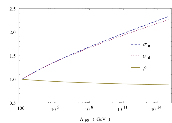
Figure 4: An illustration of the changes of $\sigma_{\rm q}$ and $\rho$ with the scale $\Lambda_{\rm FS}$ in the SM.

Note that the geometrical relation in Eq. (30) can be reexpressed as $(a_{\rm q}\tilde{b}_{\rm q}-b_{\rm q}^{2})/(\Delta_{1}+\Delta_{2})\sim m_{2}/m_{3}$. Hence in each entry of the (2,3) sector of $M_{\rm u}(M_{Z})$ the second term is suppressed by a factor proportional to $(1-\rho)\ m_{c}/m_{t}\lesssim 10^{-3}$ as compared with the first term. As for $M_{\rm d}(M_{Z})$, let us take its (2,3) entry as an example to look at the corresponding RGE correction. Because of the parallelism between $(a_{\rm u},b_{\rm u},\tilde{b}_{\rm u})$ and $(a_{\rm d},{\rm Re}(b_{\rm d}),\tilde{b}_{\rm d})$, we find

$$\Delta_{3}a_{\rm d}-\Delta_{1}{\rm Re}(b_{\rm d}) = \Delta_{1}\rm Re(b_{\rm d})\left[\displaystyle\frac{\Delta_{3}}{\Delta_{1}}\frac{a_{\rm d}}{{\rm Re}(b_{\rm d})}-1\right]$$ (100)

$$\simeq \Delta_{1}{\rm Re}(b_{\rm d})\left[\displaystyle\frac{\Delta_{3}}{\Delta_{1}}\frac{a_{\rm u}}{b_{\rm u}}-1\right]={\rm Re}(b_{\rm d})\left(a_{\rm u}\tilde{b}_{\rm u}-b_{\rm u}^{2}\right)\ .$$

So the real part of the second term of $M_{\rm d23}$ at $M_{Z}$ is suppressed by a factor proportional to $(1-\rho)\ m_{c}/m_{t}\lesssim 10^{-3}$ as compared with the real part of its first term. In other words, the real part of $M_{\rm d23}$ is approximately equal to $\rho^{-1}{\rm Re}(b_{\rm d})$ at $M_{Z}$. According to our phase assignment in Eq. (80), $\phi_{2}=\arg(b_{\rm u})-\arg(b_{\rm d})=-\arg(b_{\rm d})$ holds. Hence the phase of $b_{\rm d}$ is equal to $-\phi_{2}$ and must be close to $0$ or $-2\pi$. In the $r\sim 1$ region where $\Delta_{2}$ is much smaller than $\Delta_{1}$, it is easy to see that the imaginary part of the (2,3) entry of $M_{\rm d}(M_{Z})$ is about ${\rm Im}(b_{\rm d})$. That means $\arg(b_{\rm d})\simeq{\rm Im}(b_{\rm d})/{\rm Re}(b_{\rm d})$ is rescaled by $\rho$ due to the RGE effects, or equivalently

$$\phi_{2}(\Lambda_{\rm FS})\simeq\rho^{-1}\phi_{2}(M_{Z})\ .$$ (101)

In a word, the four texture zeros of quark mass matrices are essentially stable against the evolution of energy scales. To be more specific, $M_{\rm u}$ and $M_{\rm d}$ develop the overall factors $\sigma_{\rm u}$ and $\sigma_{\rm d}$ during their running from $\Lambda_{\rm FS}$ down to $M_{Z}$, respectively; and their finite entries $(a_{\rm u},b_{\rm u},\tilde{b}_{\rm u})$ and $(a_{\rm d},{\rm Re}(b_{\rm d}),\tilde{b}_{\rm d})$ are rescaled by $\rho$ and $\rho^{-1}$, respectively.

To illustrate the RGE-induced corrections, let us give a numerical example to compare between Eq. (80) at $\Lambda_{\rm FS}$ and Eq. (94) at $M_{Z}$. We first figure out the values of quark masses and flavor mixing parameters at $\Lambda_{\rm{FS}}\sim 10^{11}$ GeV by solving the one-loop RGEs numerically:

$$\begin{array}[]{lll}m_{u}=0.69\ {\rm MeV}\;,&\hskip 28.45274ptm_{c}=320\ {\rm MeV}\;,&\hskip 28.45274ptm_{t}=95.6\ {\rm GeV}\;;\\ m_{d}=1.4\ {\rm MeV}\;,&\hskip 28.45274ptm_{s}=29.1\ {\rm MeV}\;,&\hskip 28.45274ptm_{b}=1.3\ {\rm GeV}\;;\\ |V_{us}|=0.225\ ,&\hskip 28.45274pt|V_{cb}|=0.0458\ ,&\hskip 28.45274pt|V_{ub}|=0.00387\ ,\end{array}$$ (102)

and the value of $\sin 2\beta$ is almost unchanged from $M_{Z}$ to $\Lambda_{\rm FS}$ (or vice versa) within the accuracy that we need. The choice of this specific scale is for two simple reasons: on the one hand, it is expected to be around the canonical seesaw SS and leptogenesis FY scales; on the other hand, it is close to the energy scale relevant for the possible vacuum stability issue of the SM stability . Therefore,

$$Y_{\rm u}(\Lambda_{\rm FS}) \simeq 10^{-1}\left(\begin{array}[]{ccc}0&\hskip 2.84544pt9\times 10^{-4}&\hskip 2.84544pt0\\ \cdots&\hskip 2.84544pt0.6&\hskip 2.84544pt1.7\\ \cdots&\hskip 2.84544pt\cdots&\hskip 2.84544pt4.9\end{array}\right)\;,$$ (106)

$$Y_{\rm d}(\Lambda_{\rm FS}) \simeq 10^{-3}\left(\begin{array}[]{ccc}0&\hskip 2.84544pt0.04\ e^{-1.67\rm i}&\hskip 2.84544pt0\\ \cdots&\hskip 2.84544pt1.0&\hskip 2.84544pt2.4\ e^{0.14\rm i}\\ \cdots&\hskip 2.84544pt\cdots&\hskip 2.84544pt6.7\end{array}\right)\;.$$ (110)

In comparison, the corresponding quark mass matrices at the electroweak scale are

$$M_{\rm u}(M_{Z}) \simeq 10^{-1}\sigma_{\rm u}v\left(\begin{array}[]{ccc}\vspace{0.2cm}0&\hskip 8.5359pt9\times 10^{-4}&\hskip 8.5359pt0\\ \vspace{0.2cm}\cdots&\hskip 8.5359pt0.6\rho-8\cdot 10^{-3}\left(\rho-1\right)&\hskip 8.5359pt1.7\rho+3\times 10^{-3}\left(\rho-1\right)\\ \cdots&\hskip 8.5359pt\cdots&\hskip 8.5359pt4.9\rho-10^{-3}\left(\rho-1\right)\end{array}\right)\;,$$ (114)

$$M_{\rm d}(M_{Z}) \simeq 10^{-3}\sigma_{\rm d}v\left(\begin{array}[]{ccc}\vspace{0.2cm}0&0.04\ e^{-1.67\rm i}&0\\ \vspace{0.2cm}\cdots&1.0\rho^{-1}-\left(0.2+0.1\rm i\right)\varepsilon&2.4\rho^{-1}+0.3{\rm i}-0.04\varepsilon\\ \cdots&\left(2.4-0.3{\rm i}\right)\rho^{-1}+\left(0.05+0.04{\rm i}\right)\varepsilon&\hskip 5.69046pt6.7\rho^{-1}+\left(0.01+0.1{\rm i}\right)\varepsilon\end{array}\right)\;,\hskip 14.22636pt$$ (118)

where $\varepsilon=\rho^{-1}-1$ is a small value of ${\cal O}(0.1)$ or much smaller. This numerical exercise confirms our qualitative analysis made above. In particular, the imaginary part of the (2,3) entry of $M_{\rm d}(M_{Z})$ is really independent of $\rho$, and its real part is proportional to $\rho^{-1}$.

Now let us turn to the running behaviors of quark masses and flavor mixing parameters. Since $c_{\rm u}$ is negligibly small in magnitude as compared with $a_{\rm u}$, $b_{\rm u}$ and $\tilde{b}_{\rm u}$, the invariants of the (2,3) submatrix of $M_{\rm u}(\Lambda_{\rm FS})$ and $M_{\rm u}(M_{Z})$ lead us to

$$m_{c}(\Lambda_{\rm FS})+m_{t}(\Lambda_{\rm FS})\simeq v\left(a_{\rm u}+\tilde{b}_{\rm u}\right)\ ,$$

$$m_{c}(\Lambda_{\rm FS})\ m_{t}(\Lambda_{\rm FS})\simeq v^{2}\left(a_{\rm u}\tilde{b}_{\rm u}-b_{\rm u}^{2}\right)\ ;$$

$$m_{c}(M_{Z})+m_{t}(M_{Z})\simeq\sigma_{\rm u}v\left(a_{\rm u}+\tilde{b}_{\rm u}\right)\rho\ ,$$

$$m_{c}(M_{Z})\ m_{t}(M_{Z})\simeq\sigma_{\rm u}^{2}v^{2}\left(a_{\rm u}\tilde{b}_{\rm u}-b_{\rm u}^{2}\right)\rho\ .$$ (119)

These relations indicate that $m_{c}$ and $m_{t}$ change with the energy scale in the following way:

$$m_{t}(\Lambda_{\rm FS})\simeq\sigma_{\rm u}^{-1}\rho^{-1}m_{t}(M_{Z})\ ,\hskip 28.45274ptm_{c}(\Lambda_{\rm FS})\simeq\sigma_{\rm u}^{-1}m_{c}(M_{Z})\ .$$ (120)

When $c_{\rm u}$ is concerned, a similar trick yields $m_{u}(\Lambda_{\rm FS})\simeq\sigma_{\rm u}^{-1}m_{u}(M_{Z})$. It is easy to verify that the similar relations hold in the down sector:

$$m_{b}(\Lambda_{\rm FS})\simeq\sigma_{\rm d}^{-1}\rho\ m_{b}(M_{Z})\ ,\hskip 28.45274ptm_{s}(\Lambda_{\rm FS})\simeq\sigma_{\rm d}^{-1}m_{s}(M_{Z})\ ,$$ (121)

and $m_{d}(\Lambda_{\rm FS})\simeq\sigma_{\rm d}^{-1}m_{d}(M_{Z})$. These results clearly show that the mass ratios $m_{u}/m_{c}$ and $m_{d}/m_{s}$ are essentially free from the RGE corrections.

To see how the flavor mixing parameters evolve from $\Lambda_{\rm FS}$ down to $M_{Z}$, we take a new look at Eq. (24). Above all, the dimensionless parameters $r_{\rm u}$ and $r_{\rm d}$ are independent of the energy scale to a good degree of accuracy. The reason is simply that $m_{t}$ (or $m_{b}$) and $A_{\rm u}$ (or $A_{\rm d}$) have nearly the same running behaviors, as one can see from Eqs. (63), (71) and (72). It is also straightforward to conclude that $|V_{us}|$ is stable against the evolution of energy scales. In view of $r_{\rm u}\simeq r_{\rm d}$ and $\phi_{2}\simeq 0$, we arrive at the approximation

$$|V_{cb}|\simeq\displaystyle\sqrt{\left(1-r_{\rm u}\right)r_{\rm d}}\left|\displaystyle\frac{1}{2}\ \displaystyle\frac{\eta_{\rm d}}{r_{\rm d}}\ \displaystyle\frac{m_{s}}{m_{b}}-{\rm i}\sin{\phi_{2}}\right|\ .$$ (122)

Given Eqs. (101) and (121), the running behavior of $|V_{cb}|$ turns out to be

$$\left|V_{cb}(\Lambda_{\rm FS})\right|\simeq\rho^{-1}\left|V_{cb}(M_{Z})\right|\;.$$ (123)

With the help of this result and Eq. (24), we immediately obtain

$$\left|V_{ub}(\Lambda_{\rm FS})\right|\simeq\rho^{-1}\left|V_{ub}(M_{Z})\right|\;.$$ (124)

In addition, Eq. (28) tells us that $\beta$ is nearly scale-independent. It is easy to check that $\alpha$ and $\gamma$, the other two inner angles of the CKM unitarity triangle, are also free from the RGE corrections at the one-loop level Luo .

The above results can simply be translated into the ones for three flavor mixing angles and one CP-violating phase in the standard parametrization of the CKM matrix:

$$\begin{array}[]{ll}\theta_{12}(\Lambda_{\rm FS})\simeq\theta_{12}(M_{Z})\ ,&\hskip 28.45274pt\theta_{23}(\Lambda_{\rm FS})\simeq\rho^{-1}\theta_{23}(M_{Z})\ ,\\ \theta_{13}(\Lambda_{\rm FS})\simeq\rho^{-1}\theta_{13}(M_{Z})\ ,&\hskip 28.45274pt\delta(\Lambda_{\rm FS})\simeq\delta(M_{Z})\ .\end{array}$$ (125)

Of course, $\alpha$, $\beta$ and $\gamma$ are all the functions of $\delta$ in this parametrization. As for the Jarlskog invariant ${\cal J}=\cos\theta_{12}\sin\theta_{12}\cos^{2}\theta_{13}\sin\theta_{13}\cos\theta_{23}\sin\theta_{23}\sin\delta$ J , it is easy to arrive at ${\cal J}(\Lambda_{\rm FS})\simeq\rho^{-2}{\cal J}(M_{Z})$ in the same approximation. Such a rephasing-invariant measure of weak CP violation is actually tiny, only about $3\times 10^{-5}$ at $M_{Z}$.

Finally, let us briefly comment on a possible implication of the loss of Hermiticity of $M_{\rm d}$ running from $\Lambda_{\rm FS}$ down to $M_{Z}$. We conjecture that it might have something to do with the strong CP problem scp , which is put forward due to the unnatural smallness of the parameter $\overline{\theta}=\theta_{\rm QCD}+\theta_{\rm QFD}$. Here $\theta_{\rm QCD}$ is the coefficient of the CP-violating term in the QCD Lagrangian qcd ,

$$\mathcal{L}_{\theta}=\theta_{\rm QCD}\displaystyle\frac{g_{3}^{2}}{32\pi^{2}}G_{\mu\nu}\tilde{G}^{\mu\nu}\ ;$$ (126)

and $\theta_{\rm QFD}$ comes from the quark flavor sector,

$$\theta_{\rm QFD}=\arg\left[{\rm Det}\left(M_{\rm u}M_{\rm d}\right)\right]\ .$$ (127)

The experimental upper bound of $\overline{\theta}$ is at the $10^{-11}$ level theta , in sharp contrast with a natural value of $\mathcal{O}(1)$ from a theoretical point of view. The demand for explaining why $\overline{\theta}$ is so tiny poses the strong CP problem. An attractive solution for this problem is the Peccei-Quinn mechanism pq in which an anomalous $U(1)$ symmetry is introduced to ensure a complete cancellation between $\theta_{\rm QCD}$ and $\theta_{\rm QFD}$. Another competitive strategy is to remove $\theta_{\rm QCD}$ by imposing a spontaneously broken P or CP symmetry (e.g., in the LR symmetric model), and to keep the second term vanishing in the meantime sponcp ; sponcp2 .

Being Hermitian, the four-zero texture of quark mass matrices automatically satisfies the requirement $\arg\left[{\rm Det}\left(M_{\rm u}M_{\rm d}\right)\right]=0$ at a superhigh energy scale $\Lambda_{\rm FS}$. Nevertheless, the RGE effects can render $M_{\rm d}(M_{Z})$ non-Hermitian as shown in Eq. (94). Since the strong CP term begins to take effect at the scale of about 260 MeV where the QCD vacuum transforms, nonzero $\arg\left[{\rm Det}\left(M_{\rm d}\right)\right]$ at or below $M_{Z}$ will contribute to $\overline{\theta}$ in spite of $\arg\left[{\rm Det}\left(M_{\rm d}\right)\right]=0$ at $\Lambda_{\rm FS}$. Given the explicit form of $M_{\rm u}(M_{Z})$ and $M_{\rm d}(M_{Z})$ in Eq. (63), one may calculate its contribution to $\overline{\theta}$ as follows:

$$\theta_{\rm QFD}=\arg\left[{\rm Det}M_{\rm d}(M_{Z})\right]\simeq\arctan\left[\frac{\rho^{-1}-1}{\Delta_{1}+\Delta_{2}}\frac{\Delta_{3}\ {\rm Im}(b_{\rm d})}{a_{\rm d}\ \rho^{-1}}\right]\sim\left(1-r\right)^{2}\left(1-\rho\right)\sin{\phi_{2}}\ .$$ (128)

Although $\phi_{2}$ is very small, it cannot be exactly zero as shown in our numerical analysis. Given $r=0.9$ and $\Lambda_{\rm FS}=1$ TeV, for instance, Eq. (79) leads us to a value of ${\cal O}(10^{-5})$, much larger than the upper bound of $\overline{\theta}$. One way out of this problem is to fine-tune the value of $r$. But the possibility of $r\simeq 1$ has phenomenologically been ruled out, as discussed at the beginning of section iii@. If the parallelism between the forms of $M_{\rm u}$ and $M_{\rm d}$ is given up, the situation will change. For example, in a flavor basis with $M_{\rm u}$ being diagonal, the value of $\theta_{\rm QFD}$ was estimated to be of ${\cal O}(10^{-16})$ in Ref. qfd . In short, it seems difficult to directly employ the four-zero texture of quark mass matrices to solve the strong CP problem in the scenario of spontaneous CP violation. But a more detailed study of this issue is needed before a firm conclusion can be achieved.

V Summary

We have carried out a new study of the four-zero texture of Hermitian quark mass matrices and improved the previous works in several aspects. In our numerical analysis what really matters is that we have found a new part of the parameter space, corresponding to $A\sim|B|\sim\tilde{B}$ (or $r\sim 0.5$), and confirmed the known part corresponding to $A>|B|>\tilde{B}$ (or $r\sim 1$). In particular, the exact equality between $A$ and $\tilde{B}$ is allowed, and this opens an interesting window for model building. We want to emphasize that the newly found parameter space is phenomenologically different from the already known: since the former allows the (near) equality of mass matrix entries — a characteristic of non-Abelian flavor symmetries which are very popular in the lepton sector f-symmetry , it provides a possibility of unifying the description of quarks and leptons with the same flavor symmetries and this will be discussed elsewhere.

We have identified two special four-zero patterns of quark mass matrices and constructed two toy flavor-symmetry models to realize them. One of the patterns possesses a mild hierarchy $A\sim\epsilon|B|\sim\epsilon^{2}\tilde{B}$ with $\epsilon$ being about 0.3, and it can be obtained with the help of the FN mechanism. The other pattern assumes $A=\tilde{B}$, which can be realized by means of the $S(3)$ flavor symmetry. Both of them show a similarity between the (2,3) sectors of $M_{\rm u}$ and $M_{\rm d}$, indicating that the latter could have the same origin. We have done two model-building exercises in the SUSY LR framework with an explicit parity symmetry, which ensures the Hermiticity of quark mass matrices at the flavor symmetry scale $\Lambda_{\rm FS}$.

We have also studied the RGE effects on the four-zero texture of quark mass matrices in an analytical way, from $\Lambda_{\rm FS}$ down to the electroweak scale $M_{Z}$. Our results show that the texture zeros of $M_{\rm u}$ and $M_{\rm d}$ are essentially stable against the evolution of energy scales, but their finite entries are rescaled due to the RGE-induced corrections. An interesting consequence of the RGE running is the loss of the Hermiticity of $M_{\rm d}$ at $M_{Z}$ in the SM. As a byproduct, the possibility of applying the four-zero texture of quark mass matrices to resolving the strong CP problem has been discussed in a very brief way.

Although the predictive power of texture zeros has recently been questioned in the lepton sector Grimus , they remain useful in the quark sector to understand the correlation between the hierarchy of quark masses and that of flavor mixing angles. We remark that possible flavor symmetries are behind possible texture zeros, and they are phenomenologically important to probe the underlying flavor structure before a complete flavor theory is developed.

Note added. While our paper was being finished, we noticed a new preprint LG in which a systematic survey of possible texture zeros of quark mass matrices was done but the four-zero texture of Hermitian quark mass matrices with the up-down parallelism was not explicitly discussed.

References

(1)
G. Aad et al. (ATLAS Collaboration), Phys. Lett. B 716, 1 (2012);
S. Chatrchyan (CMS Collaboration), Phys. Lett. B 716, 30 (2012).
(2)
For a brief review, see: Z. Z. Xing, Int. J. Mod. Phys. A 29, 1430067 (2014).
(3)
N. Cabibbo, Phys. Rev. Lett. 10, 531 (1963);
M. Kobayashi and T. Maskawa, Prog. Theor. Phys. 49, 652 (1973).
(4)
R. Gatto, G. Sartori and M. Tonin, Phys. Lett. B 28, 128 (1968).
(5)
H. Fritzsch, Phys. Lett. B 73, 317 (1978);
Nucl. Phys. B 155, 189 (1979);
For a review with extensive references, see: H. Fritzsch and Z. Z. Xing,
Prog. Part. Nucl. Phys. 45, 1 (2000).
(6)
N. Mahajan, R. Verma and M. Gupta, Int. J. Mod. Phys. A 25, 2037 (2010); W. A. Ponce and R. H. Benavides, Eur. Phys. J. C
71, 1641 (2011); Y. Giraldo, Phys. Rev. D 86, 093021 (2012).
(7)
R. E. Shrock, Phys. Rev. D 45, 10 (1992); Int. J. Mod. Phys. A
7, 6357 (1992).
(8)
H. Fritzsch, Phys. Lett. B 184, 391 (1987); H. Fritzsch
and Z. Z. Xing, Phys. Lett. B 413, 396 (1997);
Phys. Rev. D 57, 594 (1998).
(9)
H. Fritzsch and Z. Z. Xing, Phys. Lett. B 555, 63 (2003).
(10)
For previous studies, see, e.g., D. Du and Z. Z. Xing, Phys. Rev. D
48, 2349 (1993); L. J. Hall and A. Rasin, Phys. Lett. B
315, 164 (1993); H. Fritzsch and D. Holtmanspotter,
Phys. Lett. B 338, 290 (1994); H. Fritzsch and
Z. Z. Xing, Phys. Lett. B 353, 114 (1995); P. S. Gill
and M. Gupta, J. Phys. G 21, 1 (1995);
Phys. Rev. D 56, 3143 (1997); H. Lehmann,
C. Newton and T. T. Wu, Phys. Lett. B 384, 249 (1996);
Z. Z. Xing, J. Phys. G 23, 1563 (1997); K. Kang and
S. K. Kang, Phys. Rev. D 56, 1511 (1997); T. Kobayashi
and Z. Z. Xing, Mod. Phys. Lett. A 12, 561 (1997); Int.
J. Mod. Phys. A 13, 2201 (1998); J. L. Chkareuli and
C. D. Froggatt, Phys. Lett. B 450, 158 (1999); J. L. Chkareuli,
C. D. Froggatt and H. B. Nielsen, Nucl. Phys. B 626, 307 (2002); A. Mondragon and
E. Rodriguez-Jauregui, Phys. Rev. D 59, 093009 (1999);
H. Nishiura, K. Matsuda and T. Fukuyama, Phys. Rev. D 60, 013006 (1999); G. C. Branco, D. Emmanuel-Costa and
R. Gonzalez Felipe, Phys. Lett. B 477, 147 (2000);
S. H. Chiu, T. K. Kuo and G. H. Wu, Phys. Rev. D 62,
053014 (2000); H. Fritzsch and Z. Z. Xing, Phys. Rev. D 61, 073016 (2000); Phys. Lett. B 506, 109 (2001);
R. Rosenfeld and J. L. Rosner, Phys. Lett. B 516, 408
(2001); R. G. Roberts, A. Romanino, G. G. Ross, and
L. Velasco-Sevilla, Nucl. Phys. B 615, 358 (2001).
(11)
For recent studies, see, e.g., R. Verma, G. Ahuja and M. Gupta,
Phys. Lett. B 681, 330 (2009); R. Verma, G. Ahuja,
N. Mahajan, M. Randhawa and M. Gupta, J. Phys. G 37,
075020 (2010); M. Gupta and G. Ahuja, Int. J. Mod. Phys. A 26, 2973 (2011); F. N. Ndili, arXiv:1205.5326 [hep-ph]; R. Verma, J. Phys.
G 40, 125003 (2013);
W. G. Hollik and U. J. S. Salazar, arXiv:1411.3549 [hep-ph].
(12)
Z. Z. Xing and H. Zhang, J. Phys. G 30, 129 (2004).
(13)
K. A. Olive et al. (Particle Data Group), Chin. Phys. C
38, 090001 (2014).
(14)
Z. Z. Xing, H. Zhang and S. Zhou, Phys. Rev. D 77,
113016 (2008); Phys. Rev. D 86, 013013 (2012).
(15)
H. Fritzsch and Z. Z. Xing, Phys. Lett. B 353, 114 (1995).
(16)
Z. Z. Xing and S. Zhou, Phys. Lett. B 737, 196 (2014);
S. Luo and Z. Z. Xing, Phys. Rev. D 90, 073005 (2014).
(17)
K. Matsuda, T. Fukuyama and H. Nishiura, Phys. Rev. D 61, 053001 (2000); H. Nishiura, K. Matsuda, T. Kikuchi and
T. Fukuyama, Phys. Rev. D 65, 097301 (2002); K. Matsuda
and H. Nishiura, Phys. Rev. D 69, 053005 (2004).
(18)
A. E. Carcamo Hernandez, R. Martinez and J. A. Rodriguez,
Eur. Phys. J. C 50, 935 (2007).
(19)
C. D. Froggatt and H. B. Nielsen, Nucl. Phys. B 147, 277
(1979).
(20)
H. Harari, H. Haut and J. Weyers, Phys. Lett. B 78, 459
(1978); M. Fukugita, M. Tanimoto and T. Yanagida, Phys. Rev. D
57, 4429 (1998); H. Fritzsch and Z. Z. Xing, Phys. Lett.
B 440, 313 (1998).
(21)
J. C. Pati and A. Salam, Phys. Rev. D 10, 275 (1974);
R. N. Mohapatra and J. C. Pati, Phys. Rev. D 11, 566
(1975); Phys. Rev. D 11, 2558 (1975); G. Senjanovic and
R. N. Mohapatra, Phys. Rev. D 12, 1502 (1975).
(22)
C. S. Aulakh, K. Benakli and G. Senjanovic, Phys. Rev. Lett.
79, 2188 (1997); R. Kuchimanchi and R. N. Mohapatra,
Phys. Rev. D 48, 4352 (1993); Phys. Rev. Lett. 75, 3989 (1995).
(23)
H. Ishimori, T. Kobayashi, H. Ohki, H. Okada, Y. Shimizu and M. Tanimoto,
Prog. Theor. Phys. Suppl. 183, 1 (2010).
(24)For a review, see G. Altarelli and F. Feruglio,
Rev. Mod. Phys. 82, 2701 (2010).
(25)
For a previous study of the RGE effects on the texture zeros of
quark mass matrices, see, e.g., Z. Z. Xing, Phys. Rev. D 68,
073008 (2003).
(26)
C. H. Albright and M. Lindner, Phys. Lett. B 213, 347 (1988).
(27)
B. Grzadkowski and M. Lindner, Phys. Lett. B 193, 71
(1987); B. Grzadkowski, M. Lindner and S. Theisen, Phys. Lett. B
198, 64 (1987).
(28) P. Minkowski, Phys. Lett. B 67, 421 (1977);
T. Yanagida, in Proceedings of the Workshop on Unified Theory
and the Baryon Number of the Universe, edited by O. Sawada and A. Sugamoto
(KEK, Tsukuba, 1979), p. 95; M. Gell-Mann, P. Ramond, and
R. Slansky, in Supergravity, edited by P. van Nieuwenhuizen
and D. Freedman (North-Holland, Amsterdam, 1979), p. 315; S. L. Glashow,
in Quarks and Leptons, edited by M. Lvy et al. (Plenum, New York, 1980), p. 707; R. N. Mohapatra
and G. Senjanovic, Phys. Rev. Lett. 44, 912 (1980).
(29) M. Fukugita and T. Yanagida, Phys. Lett. B 174,
45 (1986).
(30)
For a discussion about this issue, see, e.g., J. Elias-Miro,
J. R. Espinosa, G. F. Giudice, G. Isidori, A. Riotto and A. Strumia,
Phys. Lett. B 709, 222 (2012); and Ref. mass .
(31)
Z. Z. Xing, Phys. Lett. B 679, 111 (2009); S. Luo and Z. Z.
Xing, J. Phys. G 37, 075018 (2010).
(32)
C. Jarlskog, Phys. Rev. Lett. 55, 1039 (1985);
Z. Phys. C 29, 491 (1985).
(33)
For reviews, see, e.g., R. D. Peccei, Lect. Notes Phys. 741, 3 (2008); H. Y. Cheng, Phys. Rept. 158, 1
(1988).
(34)
C. G. Callan, R. F. Dashen and D. J. Gross, Phys. Lett. B 63, 334 (1976); R. Jackiw and C. Rebbi, Phys. Rev. Lett. 37, 172 (1976).
(35)
M. Burghoff et al., arXiv:1110.1505 [nucl-ex].
(36)
R. D. Peccei and H. R. Quinn, Phys. Rev. Lett. 38, 1440
(1977); Phys. Rev. D 16, 1791 (1977).
(37)
M. A. B. Beg and H. S. Tsao, Phys. Rev. Lett. 41, 278
(1978); H. Georgi, Hadronic Jour. 1, 155 (1978);
R. N. Mohapatra and G. Senjanovic, Phys. Lett. B 126,
283 (1978).
(38)
A. E. Nelson, Phys. Lett. B 143, 165 (1984); S. M. Barr,
Phys. Rev. Lett. 53, 329 (1984).
(39)
K. S. Babu, B. Dutta and R. N. Mohapatra, Phys. Rev. D 65,
016005 (2001).
(40)
P. O. Ludl and W. Grimus, JHEP 1407, 090 (2014);
P. M. Ferreira and L. Lavoura, Nucl. Phys. B 891, 378 (2014).
(41)P. O. Ludl and W. Grimus, arXiv:1501.04942 [hep-ph].