Effects of electron-phonon interaction on thermal and electrical transport through molecular nano-conductors

Abstract

The topic of this review is the effects of electron-phonon interaction (EPI) on the transport properties of molecular nano-conductors. A nano-conductor connects to two electron leads and two phonon leads, possibly at different temperatures or chemical potentials. The EPI appears only in the nano-conductor. We focus on its effects on charge and energy transport. We introduce three approaches. For weak EPI, we use the nonequilibrium Green’s function method to treat it perturbatively. We derive the expressions for the charge and heat currents. For weak system-lead couplings, we use the quantum master equation approach. In both cases, we use a simple single level model to study the effects of EPI on the system’s thermoelectric transport properties. It is also interesting to look at the effect of currents on the dynamics of the phonon system. For this, we derive a semi-classical generalized Langevin equation to describe the nano-conductor’s atomic dynamics, taking the nonequilibrium electron system, as well as the rest of the atomic degrees of freedom as effective baths. We show simple applications of this approach to the problem of energy transfer between electrons and phonons.

I Introduction

Electron-phonon interaction (EPI) is one of the most important many-body interactions in condensed-matter and molecular systems, responsible for a variety of phenomena, from electrical, thermal conduction, superconductivity to Raman scattering, polaron formation, just to list a fewBorn and Huang (1954); Born and Oppenheimer (1927); van Leeuwen (2004); Ziman (1960); Grimvall (1981); Sham and Ziman (1963); Hubač and Wilson (2008). Its effects on the electrical, thermal, and optical properties of bulk semiconductors and metals have been intensively studied along with the development of many-body theories and experimental techniques. Recent advances in experimental fabrication of meso- and nano-scopic structures have generated tremendous efforts in understanding the effects of EPI on transport properties of reduced-dimensional systemsGalperin et al. (2007a); Horsfield et al. (2006); Tao (2006).

Of special interest are current-induced forces and Joule heating in low-dimensional systems, especially in molecular nano-conductorsTodorov (1998); Todorov et al. (2000); Di Ventra et al. (2004); Dundas et al. (2009); Todorov et al. (2010); Lü et al. (2010, 2012); Bode et al. (2011); Abedi et al. (2010, 2013); Stipe et al. (1998); Ness and Fisher (1999); Agraït et al. (2002a); Smit et al. (2004); Sergueev et al. (2005); Viljas et al. (2005); de la Vega et al. (2006); Paulsson et al. (2005); Huang et al. (2006); Tsutsui et al. (2007); Lü and Wang (2007); Asai (2008); Lü and Wang (2009); Ioffe et al. (2008); Wu and Cao (2009); Yu et al. (2011); Ward et al. (2011); Shekhar et al. (2011); Härtle and Thoss (2011); Shekhar et al. (2012); Hützen et al. (2012); Simine and Segal (2012, 2013); Wilner et al. (2013); Bergfield and Ratner (2013); Kaasbjerg et al. (2013); Wang et al. (2013); Simine and Segal (2014). On the one hand, the electrical transport signature of EPI is an invaluable spectroscopic tool to study the structural information of molecular nano-conductorsStipe et al. (1998); Agraït et al. (2002a). On the other hand, these processes are crucial in maintaining the stability of these conductorsSmit et al. (2004), relevant to the continuous scaling down of modern electronic devices. Different theoretical approaches have been developed to study these problems, in many cases separately. Recently, it was realized that non-conservative nature of current-induced forces provides an alternative, deterministic way of energy transfer between electrons and phonons, or more generally atomic motionsDundas et al. (2009). It is fundamentally different from the stochastic Joule heating. These advances have motivated the development of methods treating current-induced forces and Joule heating on the same footingLü et al. (2010); Bode et al. (2011); Lü et al. (2012); Lü and Wang (2009).

Equally significantly, there has been an increasing interest in the thermoelectric properties of low dimensional systemsDresselhaus et al. (2007); Dubi and Di Ventra (2011); Li et al. (2012a); Yang et al. (2012a, b). A starting point of the theoretical treatment is to ignore the effect of EPI, and study the transport of electrons and phonons separately. But how important the effect of EPI is is a pertinent question, on which much of recent work is devoted toLeijnse et al. (2010); Hsu et al. (2010); Sergueev et al. (2011); Entin-Wohlman et al. (2010); Zhou et al. (2015). Here, we will look at this problem using the various approaches we have developed.

EPI is a genuine many-body interaction, the exact treatment of which is challenging, if possible at all. One natural approach is to perform perturbation calculation over a certain small parameter. In the most common multi-probe transport setup (see Fig. 1 and Sec. II), this small parameter can be chosen according to the strength of EPI. This strength can be roughly characterized by the ratio between two time scales: the first one corresponds to the phonon period, and the second one corresponds to the electron dwell timeBüttiker (1983) in the nano-conductor. If the time electrons spend in the nano-conductor is much shorter than the phonon period, the system is in the weak EPI regime. The small parameter is the EPI matrix. In the other limit, the coupling of the nano-conductor to electrodes is the small parameter, over which one can perform the perturbation expansion.

In this review, we summarize our own effort in developing and/or utilizing different theoretical approaches to study the aforementioned problems in different parameter regimes. We discuss some relevant results when possible, but we make no effort on reviewing all of them considering the huge amount of literature. The paper is organized as follows: In Sec. II, we give a brief introduction of the EPI problem starting from the Born-Oppenheimer approximation. We then introduce the system setup and Hamiltonian we use in this paper. In Sec. III, we briefly summarize our use of the nonequilibrium Green’s function (NEGF) method to study electron, phonon transport and their interaction perturbatively. We consider several applications of the method. The first one is the effects of EPI on the thermoelectric transport coefficients in a single level model. The second one is the heat transport between electrons and phonons due to EPI. The use of simple models enables us to approach the problems semi-analytically. The last example is a numerical study of the Joule heating and phonon-drag effect in carbon nanotubes. In Sec. IV, we consider the case of strong EPI using the quantum master equation (QME) approach. After reviewing the earlier work, the same thermoelectric transport model is re-visited focusing on how the strength of EPI affects the results. In Sec. V, we focus on the current-induced dynamics. Based on the Feynman-Vernon influence functional approach, we derive the semi-classical Langevin equation, taking into account the equilibrium phonon and nonequilibrium electron baths. The final section is our conclusion and remarks.

II Born-Oppenheimer approximation and electron-phonon interactions

To discuss the meaning and formulation of the electron and phonon systems and their mutual interaction, we need to start from the Born-Oppenheimer approximationBorn and Oppenheimer (1927); Born and Huang (1954). Consider an electron-ion system with a total Hamiltonian $H=P^{i}+H^{e}$, where $P^{i}$ is the kinetic energy operator for the ions, and $H^{e}=P^{e}+U$ is electron Hamiltonian with kinetic energy of the electrons, $P^{e}$, and potential energy $U=U^{ee}+U^{ei}+U^{ii}$, which includes the Coulomb interactions among the electrons and ions. Since the ions are much heavier than the electrons, one can treat the ion kinetic energy term as a small perturbation with the expansion parameterBorn and Huang (1954)

$$\left(\frac{m_{\rm e}}{m_{\rm p}}\right)^{1/4},$$ (1)

where $m_{\rm e}$ is the mass of an electron and $m_{\rm p}$ mass of an ion (assuming all have the same mass). If the ions are considered infinitely heavy, the ions will not move and the electron wavefunctions satisfy

$$H^{e}\phi_{\alpha}(x;R)=E^{e}_{\alpha}(R)\phi_{\alpha}(x;R),$$ (2)

where $x$ represents the set of all coordinates of the electrons, $R$ the positions of all the ions, and $\alpha$ is the electronic state quantum number. The eigen-functions and the eigenvalues depend on $R$ parametrically.

We assume an orthonormal set $\{\phi_{\alpha}\}$ that satisfies Eq. (2) has been obtained. To take into account the effects of the ions, we consider a trial full wavefunction in a factored form

$$\Psi(x,R)=\phi_{\alpha}(x;R)\chi_{\beta;\alpha}(R)=|\alpha\beta\rangle,$$ (3)

and consider the variational solutionvan Leeuwen (2004) of the full Hamiltonian, ${\rm min}_{\chi}\langle\Psi|H|\Psi\rangle$, subject to the normalization $\langle\chi|\chi\rangle=1$. This variational approach is equivalent to omitting the off-diagonal elements (which is the Born-Oppenheimer approximation, see Ref. Born and Huang, 1954, App. VIII), giving an equation for the ions

$$\Bigl{(}P^{i}+E^{e}_{\alpha}(R)+\langle\phi_{\alpha}|P^{i}|\phi_{\alpha}\rangle\qquad\qquad\qquad$$

$$\qquad\qquad-\frac{\hbar^{2}}{m_{\rm p}}\langle\phi_{\alpha}|\nabla_{R}|\phi_{\alpha}\rangle\cdot\nabla_{R}\Bigr{)}\chi=E\chi,$$ (4)

where $\langle\cdots\rangle$ means the $x$-dependence is integrated out but still $R$-dependent; $\nabla_{R}$ is a multi-dimensional gradient operator with respect to $R$. Since the left-hand side depends on the electronic quantum number $\alpha$, the full eigen-energy $E$ and functions also depend on $\alpha$ parametrically, e.g., we may write $E_{\beta;\alpha}$.

If we assume that the electrons are in its instantaneous ground state, the ions move in a potential surface generated by the electrons. There are no explicit electron-phonon interaction (EPI) terms. To account for the EPI, we need to go back to the basis, Eq. (3), and consider the matrix elements

$$\langle\alpha\beta|H|\alpha^{\prime}\beta^{\prime}\rangle.$$ (5)

The off-diagonal terms are interpreted as the EPIZiman (1960); Grimvall (1981), which are small. If the off-diagonals are omitted, the electrons stay in a given quantum state $\alpha$. The off-diagonal terms describe the scattering of the electrons to different state $\alpha^{\prime}$. If ion displacements are small, the most important contribution is from the linear term in the displacement

$$-\frac{\hbar^{2}}{m_{\rm p}}\langle\phi_{\alpha}\chi_{\beta;\alpha}|\nabla_{R}|\phi_{\alpha^{\prime}}\rangle\cdot\nabla_{R}|\chi_{\beta^{\prime};\alpha^{\prime}}\rangle,\quad(\alpha,\beta)\neq(\alpha^{\prime},\beta^{\prime}).$$ (6)

These off-diagonal matrix elements can be used, e.g., in a Fermi-Golden rule calculation of scattering processes. However, the identity (in the sense of effective Hamiltonians) of the electrons and phonons and their mutual interaction are not at all clear. Although EPI plays major role in many physical processesSham and Ziman (1963), such as electronic transport and superconductivity, its conceptual foundation is still not very solid. Within the Born-Oppenheimer scheme, it is not clear at all how to transform the original Hamiltonian $H$ into a form of an electron system and independent phonon system and their interaction unambiguously. The problem is related to the fact that in deriving the phonon Hamiltonian (the potential surfaces), the effect of electrons is already used. Thus, putting the electrons back amounts to double counting, see Refs. van Leeuwen, 2004; Hubač and Wilson, 2008 for some of the modern treatments.

Instead of pursuing a self-consistent theory of EPI from the Born-Oppenheimer approximation, here in this review, and also in many of the practical applicationsDeegan (1972); Ashkenazi and Dacorogna (1981); Cappelluti and Pietronero (2006); Frederiksen et al. (2007); Giustino et al. (2007), we adopt a phenomenological point of view, and use the model Hamiltonians as given below in Eqs. (8) and (10). Focusing only the term linear in the displacements away from the equilibrium positions of the ions, we can think of the single electron Hamiltonian $H_{\rm e}$ below having a $R$-dependence. Taylor expanding it, $R=R^{0}+u/\sqrt{m_{\rm p}}$, we obtain

$$M_{ij}^{k}=\frac{1}{\sqrt{m_{\rm p}}}\,\langle i|\frac{\partial H_{\rm e}(R)}{\partial R_{k}}|j\rangle,$$ (7)

where $|j\rangle$ is the single particle state when ionic system is in equilibrium position $R^{0}$. The extra factor of square root of ion mass $m_{\rm p}$ is because of our convention of displacement variable $u$. This form of interaction is intuitively understandable and originally proposed by BlochBloch (1928). In Chap. 4 of Ref. Grimvall, 1981, a derivative from Eq. (6) to (7) is given, but the reasoning does not seem to be rigorous.

Thus, our starting point of a derivation is a tight-binding Hamiltonian for the electrons, harmonic couplings for the phonons and a standard EPI term. They are taken as given and exact. The charge redistributions and self-consistency for the electrons are not part of the discussion. Symbolically, the total many-body Hamiltonian is given as

$$H_{{\rm tot}}=H^{0}_{{\rm e}}+H_{{\rm p}}+H_{{\rm ep}},$$ (8)

where the electron part is $H^{0}_{{\rm e}}=c^{\dagger}Hc$, the phonon part $H_{{\rm p}}=\frac{1}{2}(p^{T}p+u^{T}Ku)+V_{n}(u^{C})$. The variable $u$ is mass normalized, $u_{j}=\sqrt{m_{j}}(R_{j}-R_{j}^{0})$. Because of this, the conjugate momentum is $p=\dot{u}$. $V_{n}$ is the nonlinear force contribution. $c$ is a column vector of the electron annihilation operators, which we can separate into three regions, the left, center, and right, $c=(c^{L},d,c^{R})^{T}$, $T$ stands for matrix transpose. Similarly $u=(u^{L},u^{C},u^{R})^{T}$. Accordingly, the matrices $H$ and $K$ are partitioned into nine regions (submatrices), e.g.,

$$H=\left(\begin{array}[]{ccc}H^{L}&H^{LC}&0\\ H^{CL}&H^{C}&H^{CR}\\ 0&H^{RC}&H^{R}\end{array}\right),$$ (9)

such that $H^{0}_{\rm e}=H_{\rm e}^{L}+H_{\rm e}^{R}+H_{\rm e}^{C}+V_{\rm e}$, with $V_{\rm e}=V_{\rm e}^{L}+V_{\rm e}^{R}$, $V_{\rm e}^{L}={c^{L}}^{\dagger}H^{LC}d+{\rm H.c.}$. Note that we assume no interaction between the left and right leads (See Ref. Li et al., 2012b for transport when there is a lead-lead coupling). We do a similar partitioning for $K$ using the notation of Ref. Wang et al., 2008. The EPI takes the form

$$H_{{\rm ep}}(d,u^{C})=\sum_{ijk}M_{ij}^{k}u^{C}_{k}d_{i}^{\dagger}d_{j}=\sum_{k}u^{C}_{k}d^{\dagger}M^{k}d.$$ (10)

We assume that the EPI appears only in the central region. A schematic representation of the system setup is shown in Fig. 1.

The separation of the electron and phonon leads makes the theoretical development easier. In reality, they could either be physically separated, or built into one. For example, one electrode could serve both as an electron and a phonon lead, but we assume that we have independent control over their temperatures $T^{\alpha}_{\rm e}$ and $T^{\alpha}_{\rm p}$, $\alpha=L,R$.

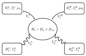
Figure 1: Model system considered in this review. The center device, including both electrons, phonons, and their interactions, is coupled with two electron and two phonon leads. Each electron lead is characterized by its chemical potential $\mu_{\alpha}$ and temperature $T^{\alpha}_{\rm e}$, and each phonon lead by temperature $T^{\alpha}_{\rm p}$.

III Weak EPI regime: Nonequilibrium Green’s function method

III.1 Theory

We first consider the case where EPI is weak, so that we can perform a perturbation expansion over the interaction matrix $M$. In order to do so, we use the NEGF method. Detailed introduction is given in our previous workWang et al. (2008, 2014); Lü and Wang (2007, 2008). This section can be considered as an application of the general approach developed in Refs. Wang et al., 2008-Wang et al., 2014 to the EPI problem. We use similar notations therein, and only give a brief outline of the approach here.

We denote the electron device Green’s function without and with EPI by $G_{0}$ and $G$, the corresponding phonon Green’s functions by $D_{0}$ and $D$, and the lead Green’s functions without coupling to the center as $g_{\alpha}$ and $d_{\alpha}$, respectively. The couplings of the device with the leads and that between the electrons and phonons are described by self-energies, with $\Sigma$ and $\Pi$ representing that of electron and phonon, respectively. For example, we define the time-ordered electron Green’s function including EPI on the Keldysh contour [Fig. 14 (b)]

$$G_{ij}(\tau,\tau^{\prime})=-\frac{i}{\hbar}\langle{T}_{C}c_{i}(\tau)c^{\dagger}_{j}(\tau^{\prime})\rangle.$$ (11)

Here, $\tau/\tau^{\prime}$ is time on the contour, and $i/j$ is index of the electronic states. The contour time order operator $T_{C}$ puts the operators later in the contour to the left. The average $\langle\cdot\rangle$ is with respect to the density matrix of the full Hamiltonian.

The contour ordered Green’s function can be divided into different groups according to the spatial position of $i/j$, similar to the Hamiltonian. The most interesting one is $G^{C}$, where $i$ and $j$ are both at the center device region. At the same time, it can be written as a $2\times 2$ matrix in time space

$$G(\tau_{i},\tau_{j})=\left(\begin{array}[]{cc}G^{t}(t_{i},t_{j})&G^{<}(t_{i},t_{j})\\ G^{>}(t_{i},t_{j})&G^{\bar{t}}(t_{i},t_{j})\end{array}\right),$$ (12)

with $G^{t}$, $G^{\bar{t}}$, $G^{>}$, $G^{<}$ the time-ordered, anti-time-ordered, greater and lesser Green’s functions. The retarded and advanced Green’s functions are obtained from them, i.e., $G^{r}=G^{t}-G^{<}$, and $G^{a}=G^{<}-G^{\bar{t}}$. For the definition and relations among these Green’s functions, we refer to the book by Haug and JauhoHaug and Jauho (2008), and our previous publicationsLü and Wang (2007); Wang et al. (2008, 2014).

To calculate the Green’s functions, we use a process of two-step adiabatic switch on. We start from the decoupled system and leads. Each of the electron and phonon leads is at its own equilibrium state, characterized by the temperature $T^{\alpha}$ and/or chemical potential $\mu_{\alpha}$. The corresponding equilibrium Green’s functions can thus be defined according to the equilibrium canonical distribution. The initial state of the system is arbitrary and not important in most cases (e.g., for steady state).

At the first step, we switch on the interaction of the center Hamiltonian with the electron and phonon leads. We wait until the electron and phonon subsystem reaches their own nonequilibrium steady state, since the temperature and/or chemical potential of each lead can be different. The two subsystems are quadratic and exactly solvable, and we get the non-interacting center Green’s functions $G_{0}$ and $D_{0}$ from the Dyson equation (we omit the superscript $C$)

$$G_{0}(1,2) = g_{C}(1,2)+g_{C}(1,3)\Sigma_{\rm b}(3,4)G_{0}(4,2),$$ (13)

$$D_{0}(1,2) = d_{C}(1,2)+d_{C}(1,3)\Pi_{\rm b}(3,4)D_{0}(4,2).$$ (14)

Here, we have used a single number to represent the matrix indices and contour time arguments, i.e., $G_{0}(1,2)={G_{0}}_{j_{1}j_{2}}(\tau_{1},\tau_{2})$. Summation or integration over repeated indices is assumed. $g_{C}$ ($d_{C}$) is the center electron (phonon) Green’s function without coupling to the $L$ and $R$ leads. The self-energy $\Sigma_{\rm b}=\Sigma_{L}+\Sigma_{R}$ includes contributions from $L$ and $R$, with $\Sigma_{\alpha}(1,2)=H^{C\alpha}g_{\alpha}(1,2)H^{\alpha C}$; similarly for $\Pi_{\rm b}$.

At the second step, we adiabatically switch on the EPI in the center. We perform a perturbation expansion over the interaction Hamiltonian $H_{\rm ep}$, using Feynman diagramatics. The interacting Green’s functions are expressed using similar Dyson equations as Eqs. (13-14),

$$G(1,2) = G_{0}(1,2)+G_{0}(1,3)\Sigma_{\rm ep}(3,4)G(4,2),$$ (15)

$$D(1,2) = D_{0}(1,2)+D_{0}(1,3)\Pi_{\rm ep}(3,4)D(4,2).$$ (16)

Here, $\Sigma_{\rm ep}$ and $\Pi_{\rm ep}$ are electron and phonon self-energies due to EPI. Using Eq. (12), at steady state, we can get the following useful relations in energy/frequency domain

$$G^{r}(\varepsilon) = \left[(\varepsilon+i0^{+})I-H^{C}-\Sigma^{r}_{\rm tot}(\varepsilon)\right]^{-1},$$ (17)

$$D^{r}(\omega) = \left[(\omega+i0^{+})^{2}I-K^{C}-\Pi^{r}_{\rm tot}(\omega)\right]^{-1},$$ (18)

$$\Sigma^{r}_{\rm tot}(\varepsilon) = \Sigma^{r}_{\rm b}(\varepsilon)+\Sigma^{r}_{\rm ep}(\varepsilon),$$ (19)

$$\Pi^{r}_{\rm tot}(\omega) = \Pi^{r}_{\rm b}(\omega)+\Pi^{r}_{\rm ep}(\omega).$$ (20)

We use $\varepsilon$ for the energy of electron and $\omega$ for the angular frequency of phonon, respectively, and $I$ is the identity matrix. To get an expression for the current, we also need the greater and lesser version of the Green’s functionsHaug and Jauho (2008)

$$G^{>,<}(\varepsilon) = G^{r}(\varepsilon)\Sigma_{\rm tot}^{>,<}(\varepsilon)G^{a}(\varepsilon),$$ (21)

$$D^{>,<}(\omega) = D^{r}(\omega)\Pi_{\rm tot}^{>,<}(\omega)D^{a}(\omega).$$ (22)

The electrical current ($I_{\rm e}$) is expressed as the change rate of the electron number in one of the leads ($N^{\alpha}$) times the charge of electron ($-e$). For example,

$$I_{\rm e} = -e\langle\frac{dN^{L}(t)}{dt}\rangle$$ (23)

$$= -\frac{2e}{\hbar}{\rm Im}{\rm Tr}\left[V^{LC}_{\rm e}\langle{c^{L}}^{\dagger}(t)d(t)\rangle\right]$$

$$= 2e{\rm Re}{\rm Tr}\left[V^{LC}_{\rm e}G^{<,CL}(t=0)\right].$$

It can be expressed by the Green’s function of the center region and the lead self-energiesMeir and Wingreen (1992); Jauho et al. (1994); Haug and Jauho (2008),

$$I_{\rm e}=\frac{e}{\hbar}\int_{-\infty}^{+\infty}\frac{d\varepsilon}{2\pi}{\rm Tr}\left[G^{>}\Sigma_{L}^{<}-G^{<}\Sigma_{L}^{>}\right].$$ (24)

Similarly for the heat current carried by electrons ($I_{\rm h}$) and phonons ($I_{\rm p}$)

$$I_{\rm h} = \frac{1}{\hbar}\int_{-\infty}^{+\infty}\frac{d\varepsilon}{2\pi}(\varepsilon-\mu_{L}){\rm Tr}\left[G^{>}\Sigma_{L}^{<}-G^{<}\Sigma_{L}^{>}\right],$$ (25)

$$I_{\rm p} = -\int_{-\infty}^{+\infty}\frac{d\omega}{4\pi}\hbar\omega{\rm Tr}\left[D^{>}\Pi^{<}_{L}-D^{<}\Pi^{>}_{L}\right].$$ (26)

We have defined the positive current direction as electrons going from the lead to the center. We dropped the argument of the Green’s functions for simplicity. We ignore the spin degrees of freedom, since it is not relevant here. Currents out of the right lead are obtained by replacing index $L$ by $R$. One can symmetrize the expressions based on energy and charge conservation.

The set of coupled equations Eqs. (17-22) is difficult to solve, due to the many-body EPI. Since the EPI is weak, we consider only the lowest order Feynman diagrams shown in Fig. 2. The expressions for the self-energies are as follows. The electron Fock self-energies from phonons are

$$\Sigma_{mn}^{F,<,>}(\varepsilon) = i\hbar\int M^{k}_{mi}G^{<,>}_{0,ij}(\varepsilon_{-})D^{<,>}_{0,kl}(\omega)M^{l}_{jn}\frac{d\omega}{2\pi},$$

$$\Sigma_{mn}^{F,r}(\varepsilon) = i\hbar\int M^{k}_{mi}\bigl{(}G^{r}_{0,ij}(\varepsilon_{-})D^{<}_{0,kl}(\omega)\bigr{.}$$ (28)

$$+ \bigl{.}G^{>}_{0,ij}(\varepsilon_{-})D^{r}_{0,kl}(\omega)\bigr{)}M^{l}_{jn}\frac{d\omega}{2\pi}.$$

The Hartree self-energy does not depend on energy

$$\Sigma_{mn}^{r} = -iM_{mn}^{i}D^{r}_{ij}(\omega=0)\int M_{kl}^{j}G^{<}_{lk}(\varepsilon)\frac{d\varepsilon}{2\pi}.$$ (29)

The phonon self-energies from electrons are

$$\Pi^{<,>}_{mn}(\omega)=-i\int\frac{d\varepsilon}{2\pi}{\rm Tr}\left[M^{m}G_{0}^{<,>}(\varepsilon)M^{n}G_{0}^{>,<}(\varepsilon_{-})\right],$$ (30)

$$\Pi^{r,a}_{mn}(\omega) = -i\int\frac{d\varepsilon}{2\pi}{\rm Tr}\left[M^{m}G_{0}^{r,a}(\varepsilon)M^{n}G_{0}^{<}(\varepsilon_{-})\right.$$ (31)

$$+\left.M^{m}G_{0}^{<}(\varepsilon)M^{n}G_{0}^{a,r}(\varepsilon_{-})\right],$$

with $\varepsilon_{-}=\varepsilon-\hbar\omega$. Summation over repeated indices is assumed here. Different charge and energy conserving approximations have been developed in the literature. We will use two of them. In Subsec. III.2, we perform an expansion of the current up to the second order in $M$, following the idea of Ref. Paulsson et al., 2005. In the numerical model calculation in Subsec. III.3, we use the self-consistent Born approximation (SCBA), which means we replace $G_{0}$, $D_{0}$ by $G$, $D$ respectively in the above equations.

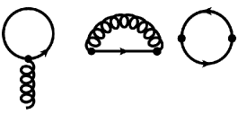
Figure 2: Feynman diagrams due to electron-phonon interaction. The first two are Hartree and Fock diagram for electrons, and the last one is the polarization bubble for phonons. The expressions of these diagrams can be found in Eqs. (III.1-31).

III.2 Thermoelectric transport through a single electronic level

We consider a single electronic level $H^{C}_{\rm e}=\varepsilon_{0}d^{\dagger}d$, coupled to the left and right electrodes, characterized by the constant level-width broadening $\Gamma_{\alpha}$ with energy cutoff $\varepsilon_{D}$ (see Eq. (40) for the general definition). It interacts with an isolated phonon mode with frequency $\omega_{0}$, and $H_{\rm ep}=m_{0}d^{\dagger}du$. In the linear regime, we introduce an infinitesimal change of the chemical potential or temperature at lead $L$, e.g., $\mu_{L}=\mu+\delta\mu$, $T_{\sigma}^{L}=T+\delta T_{\sigma}$, with $\sigma=$ e or p, $\mu$ and $T$ are the corresponding equilibrium values. We look at the response of the charge and heat current due to this small perturbation. The result, up to the 2nd order in $M$, is summarized as follows,

$$\left(\begin{array}[]{cc}\frac{I_{\rm e}}{e}\\ I_{\rm h}\\ \end{array}\right)=\left(\begin{array}[]{ccc}\mathcal{L}_{0}&\mathcal{L}_{1}\\ \mathcal{L}_{1}&\mathcal{L}_{2}\end{array}\right)\left(\begin{array}[]{ccc}\delta\mu\\ \frac{\delta T_{\rm e}}{T}\end{array}\right).$$ (32)

The linear conductance and the Seebeck coefficient are

$$G_{\rm e} = e^{2}\mathcal{L}_{0},$$ (33)

$$S \equiv -\frac{\delta V}{\delta T}=-\frac{\mathcal{L}_{1}}{e\mathcal{L}_{0}T}.$$ (34)

The coefficients $\mathcal{L}_{n}$ are

$$\mathcal{L}_{n} = \sum_{i=1}^{3}\mathcal{L}^{(i)}_{n},$$ (35)

with

$$\mathcal{L}^{(1)}_{n} = \frac{1}{\hbar}\int\frac{d\varepsilon}{2\pi}(\varepsilon-\mu)^{n}\left(A_{\bar{\alpha}}\Gamma_{\alpha}\right)f^{\prime},$$ (36)

$$\mathcal{L}^{(2)}_{n} = \frac{1}{\hbar}\int\frac{d\varepsilon}{2\pi}(\varepsilon-\mu)^{n}\left(\Delta A^{\prime}_{\bar{\alpha}}\Gamma_{\alpha}\right)f^{\prime},$$ (37)

$$\mathcal{L}^{(3)}_{n} = \frac{1}{\hbar}\int\frac{d\varepsilon}{2\pi}(\varepsilon-\mu)^{n}\left(\Delta A^{\prime\prime}_{\bar{\alpha}}\Gamma_{\alpha}+2G_{0}^{r}{\rm Im}\Sigma_{\rm ep}^{r}G_{0}^{a}\Gamma_{\alpha}\right)f^{\prime}.$$

We have defined

$$f^{\prime} = -\frac{\partial f}{\partial\varepsilon},$$ (39)

$$\Gamma_{\alpha} = i\left(\Sigma_{\alpha}^{r}-\Sigma_{\alpha}^{a}\right),$$ (40)

$$A_{\alpha} = G_{0}^{r}\Gamma^{e}_{\alpha}G_{0}^{a},$$ (41)

$$\Delta A^{\prime}_{\bar{\alpha}} = G^{r}_{0}{\rm Re}\Sigma_{\rm ep}^{r}A_{\bar{\alpha}}+A_{\bar{\alpha}}{\rm Re}\Sigma_{\rm ep}^{a}G_{0}^{a},$$ (42)

$$\Delta A^{\prime\prime}_{\bar{\alpha}} = iG^{r}_{0}{\rm Im}\Sigma_{\rm ep}^{r}A_{\bar{\alpha}}+iA_{\bar{\alpha}}{\rm Im}\Sigma_{\rm ep}^{a}G_{0}^{a},$$ (43)

and $\bar{\alpha}$ means the lead different from $\alpha$. $\mathcal{L}^{(1)}_{n}$ is the single electron Landauer result. $\mathcal{L}^{(2)}_{n}$ is the quasi-elastic term. $\mathcal{L}^{(3)}$ is the inelastic term. $f$ is the Fermi-Dirac distribution function

$$f_{\alpha}(\varepsilon) = \left[{\rm exp}\left({\frac{\varepsilon-\mu_{\alpha}}{k_{B}T^{\alpha}}}\right)+1\right]^{-1}.$$ (44)

Since we are looking at the linear response regime, $f_{L}=f_{R}$, we dropped the subscript in Eq. (39). We will also use the Bose-Einstein distribution later

$$n_{B}(\omega,T) = \left[{\rm exp}\left(\frac{\hbar\omega}{k_{B}T}\right)-1\right]^{-1}.$$ (45)

When there is no ambiguity, we will also drop the argument $T$.

In the following, we set the position of the electronic level to $\varepsilon_{0}=0$, and look at the dependence of the conductance on the chemical potential $\mu$. We firstly write down the expressions for the self-energies, and make some observations based on their functional forms.

The Hartree self-energy is real and does not depend on energyLü and Wang (2007)

$$\Sigma^{r}_{H} = -\sum_{\alpha}\frac{m_{0}^{2}\Gamma_{\alpha}}{2\pi\omega_{0}^{2}}\int_{-\varepsilon_{D}}^{\varepsilon_{D}}\frac{f_{\alpha}(\varepsilon)}{\varepsilon^{2}+\Gamma^{2}/4}d\varepsilon.$$ (46)

At $T=0$, we get

$$\Sigma^{r}_{H} = -\sum_{\alpha}\frac{m_{0}^{2}\Gamma_{\alpha}}{\pi\omega_{0}^{2}\Gamma}\left.{\rm tan}^{-1}\frac{2\varepsilon}{\Gamma}\right|_{-\varepsilon_{D}}^{\mu_{\alpha}},$$ (47)

with $\Gamma=\Gamma_{L}+\Gamma_{R}$. For large enough $\varepsilon_{D}$, the lower limit term turns to $-m_{0}^{2}/(2\omega_{0}^{2})$, which is the polaron energy shift. Note here that the $1/2$ is due to the fact we use $u_{k}^{C}$ in our definition of $H_{\rm ep}$ (Eq. 10). This is different from the common definition that uses the creation and annihilation operatore $a^{\dagger}+a$ (Eq. 74). We have subtracted the polaron shift term in the following calculation, since it is a constant. After this subtraction, $\Sigma^{r}_{H}$ is odd in $\mu$ with a negative slope near $\mu=0$. We focus on the $\mu>0$ regime. It saturates to $-m_{0}^{2}/(2\omega_{0}^{2})$ for large $\mu$, e.g., $\mu\gg\Gamma$. At non-zero temperature, the slope and the saturation value change, but the shape of the curve is similar to the $T=0$ case. This means that, the Hartree term shifts the electronic level, and reduces the conductance. On the other hand, when $\mu\gg\Gamma$, the conductance tends to zero, whether we include the EPI or not. Thus, the correction to the conductance due to the Hartree term $\Delta G_{eH}\leq 0$. It starts from zero at $\mu=0$, goes back to zero at $\mu\gg\Gamma$, and it reaches a maximum magnitude at some point in the middle. The described behaviour is schematically shown in Fig. 3 (a). This effectively reduces the broadening of the single level spectral function, also the conductance peak. Since the Seebeck coefficient is related to the logarithmic derivative of the conductance, we expect it to increase the magnitude of the Seebeck coefficient near resonance, and to reduce it off resonance [Fig. 4].

The imaginary part of the retarded Fock self-energy isLü and Wang (2007)

$${\rm Im}\Sigma_{F}^{r}(\varepsilon) = -\frac{m_{0}^{2}}{4\omega_{0}}\sum_{\alpha,s=\pm}sA_{\alpha}(\varepsilon-s\hbar\omega_{0})$$ (48)

$$\times\bigl{[}1+n_{B}(s\omega_{0})-f_{\alpha}(\varepsilon-s\hbar\omega_{0})\bigr{]}.$$

It is negative and even in $\varepsilon$. Its role on the differential conductance at the phonon threshold ($eV=\hbar\omega_{0}$) has been discussed extensivelyPaulsson et al. (2008); Tal et al. (2008); Egger and Gogolin (2008); Entin-Wohlman et al. (2009). The main conclusions are: it reduces the differential conductance at $eV=\hbar\omega_{0}$ for resonant case ($\mu\sim 0$), where the bare transmission without EPI ($T_{0}\sim 1$), while it does the opposite for far off resonance case ($\mu\gg\Gamma$), where $T_{0}\to 0$. The transition point between the two opposite behaviors is $T_{0}=1/2$ if the electronic density of state (DOS) is flat. But, in general, it depends on the system parameters. At non-zero temperature, the sharp threshold broadens out, and the linear conductance is affected: its correction to the conductance $\Delta G_{eFI}$ is negative for $\mu\sim 0$, and positive for $\mu\gg\Gamma$ [Fig. 3 (c)].

Physically, ${\rm Im}\Sigma_{F}^{r}$ gives rise to phonon scattering processes. Its effect can be understood as follows: At $T=0$, for small bias ($eV<\hbar\omega_{0}$), phonon emission is not possible due to Pauli blocking, while phonon adsorption is not possible due to zero phonon population. So, ${\rm Im}\Sigma_{F}^{r}$ does not affect the linear conductance. At high enough temperature, both phonon emission and adsorption are possible even at small bias, due to the broadening of the Fermi distribution, and finite population of phonon modes. The phonon scattering process decreases the conductance on resonance, but increases it far off resonance. As a result, the Seebeck coefficient becomes smaller.

The real part ${\rm Re}\Sigma^{r}_{F}(\varepsilon)$ is obtained by the Hilbert transform of the imaginary part. At zero temperature, it diverges logarithmically at $\varepsilon-\mu=\pm\hbar\omega_{0}$Entin-Wohlman et al. (2009). Its effects on the conductance and Seebeck coefficient are difficult to analyze. We rely on the numerical result [Fig. 3 (b)].

Figure 3 shows the correction to the linear conductance of different self-energy terms as a function of $\mu$. These numerical results confirm our qualitative analysis. By comparing the total conductance at low [Fig. 3 (e)] and high temperature [Fig. 3 (f)], we see that, (1) the Hartree term dominates at low temperature, and the $G_{e}$-$\mu$ peak becomes narrower. (2) the Fock term becomes important at high temperature, and the $G_{e}$-$\mu$ peak broadens out. Their effects on the Seebeck coefficient ($S$) are shown in Fig. 4. At low temperature, when the EPI is included, the magnitude of $S$ gets larger for $\mu\sim 0$, and smaller for $|\mu|\gg\Gamma$. At high temperature, the effect of the Fock term results in drop of $S$. In any case, the correction to $S$ is small for weak EPI. But for the case of strong EPI, the correction could be large (see Subsec. IV.3).

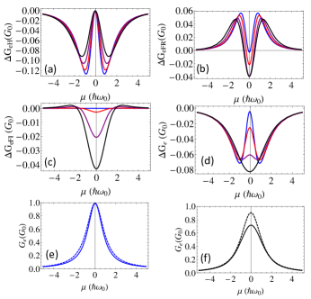
Figure 3: Chemical potential dependence of the conductance correction due to the $\Sigma^{r}_{H}(a)$, ${\rm Re}\Sigma^{r}_{F}(b)$, ${\rm Im}\Sigma^{r}_{F}(c)$, and the sum of them ($d$). The blue, red, purple, and black lines correspond to $k_{B}T=0.05,0.15,0.25,0.35\hbar\omega_{0}$, respectively. (e)-(f) The electrical conductance as a function of chemical potential ($\mu$) at $k_{B}T=0.05\hbar\omega_{0}$ (e) and $k_{B}T=0.35\hbar\omega_{0}$ (f). Solid lines include EPI, while the dashed lines do not. Other parameters used: $\Gamma_{L}=\Gamma_{R}=\hbar\omega_{0}=1$, $m_{0}=1\hbar\omega_{0}$/(Å$\sqrt{\rm{u}})$.

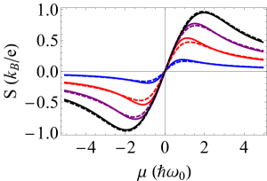
Figure 4: Change of the Seebeck coefficient due to EPI at different temperatures. The parameters and meaning of colors are the same as Fig. 3.

III.3 Heat transport between electrons and phonons

Let us look back at the setup in Fig. 1. We want to study the heat transport between electrons and phonons at finite temperature bias, but zero voltage bias. The simplest setup is that the system couples to one electron and one phonon lead, each at its own temperature, see Fig. 5. The expression for the energy current from electrons to phonons can be obtained from Eq. (26) and the expressions of the self-energies Eqs. (III.1-31)Lü and Wang (2007)

$$Q = i\hbar\int\frac{d\varepsilon}{2\pi}\int\frac{d\omega}{2\pi}\omega\left[G^{>}_{nm}(\varepsilon)M_{mi}^{k}D_{kl}^{<}(\omega)G^{<}_{ij}(\varepsilon_{-})M_{jn}^{l}\right],$$

where, again, summation over repeated indices is assumed. For the ease of analysis, we perform an expansion of the above expression to 2nd order in $M$, and it becomes

$$Q^{(2)} = \hbar\int_{0}^{+\infty}\frac{d\omega}{2\pi}\omega{\rm Tr}\bigl{[}\Lambda(\omega,T_{\rm e})\mathcal{A}(\omega)\bigr{]}$$ (50)

$$\times\bigl{[}n_{B}(\omega,T_{\rm e})-n_{B}(\omega,T_{\rm p})\bigr{]},$$

where

$$\Lambda(\omega,T_{\rm e}) = \int\frac{d\varepsilon}{2\pi}{\rm Tr}\bigl{[}MA(\varepsilon)MA(\varepsilon_{-})\bigr{]}$$ (51)

$$\times \bigl{[}f(\varepsilon,T_{\rm e})-f(\varepsilon_{-},T_{\rm e})\bigr{]},$$

and

$$\mathcal{A}(\omega) = i\bigl{[}D_{0}^{r}(\varepsilon)-D_{0}^{a}(\varepsilon)\bigr{]}.$$ (52)

Now the question we ask is whether there is a diode behaviour for the heat transport between electrons and phononsLi et al. (2012a), e.g., $Q(\Delta T)\neq Q(-\Delta T)$, with $\Delta T=T_{\rm e}-T_{\rm p}$. This is relevant because in some special situation, e.g., at metal-insulator interface, or insulating molecular junctions, EPI becomes the bottleneck of heat transferMajumdar and Reddy (2004); Segal (2008); Ren and Zhu (2013); Zhang et al. (2013); Vinkler-Aviv et al. (2014). We can define the rectification ratio as

$$R=\frac{Q(\Delta T)+Q(-\Delta T)}{Q(\Delta T)-Q(-\Delta T)}.$$ (53)

If we assume a constant electron DOS, $\Lambda(\omega)$ does not depend on $T$, we get $Q(-\Delta T)=-Q(\Delta T)$, and $R=0$. The physical reason is that in this case, it is possible to map the electron-hole pair excitation into harmonic oscillatorsTomonaga (1950); Luttinger (1963); Segal (2008). Then, it is equivalent to heat transport within a two-terminal harmonic system. We do not expect any rectification effect. To make $R\neq 0$, the electronic DOS has to be energy-dependent within the broadening of the Fermi-Dirac distribution given by $k_{B}\Delta T$. This effectively introduces anharmonicity into the system, consistent with previous studiesSegal (2008); Ren and Zhu (2013); Zhang et al. (2013).

We can go one step further, by making a Taylor expansion of the spectral function $A(\varepsilon)$ about the Fermi energy, we find that the sign of $R$ is determined by the sign of $\frac{\partial^{2}A}{\partial\varepsilon^{2}}$ (The 1st order term is zero).

Figure 5: The model system we consider to study the energy transport between electrons and phonons.

To check this argument, we calculated the heat current across one-dimensional (1D) metal-insulator junction. The metal side is represented by a 1D tight-binding chain, with hopping element $t=-0.1$ eV, and onsite energy $\varepsilon_{0}=0$. The insulator side is represented by a 1D harmonic chain with the spring constant $K=0.1$ eV/(Ųu). The insulator and metal couple through their last two degrees of freedom. Their interaction matrices are

$$M^{k}=(-1)^{k}m_{0}\left(\begin{array}[]{cc}0&1\\ 1&0\end{array}\right),\quad k=1,2.$$ (54)

Here, $m_{0}=0.05$ eV/(Å$\sqrt{\rm{u}}$), $k$ represents the phononic degrees of freedom. This means that the system couples to only one electron and one phonon lead [Fig. 5]. Figure 6 summarizes our result. In Fig. 6 (a), we show the energy current as a function of temperature difference between the metal and insulator ($\Delta T$), at two Fermi levels ($\mu=0,0.1$ eV). The energy current is asymmetric with respect to the sign change of $\Delta T$. But the rectification ratio $R$ has opposite sign. This is further highlighted in the plot of the energy current and the rectification ratio $R$ as a function of $\mu$ for fixed temperature bias $\Delta T=\pm 300$ K [Fig. 6 (b) and (c), respectively]. The sign of $R$ is well correlated with the sign of $\frac{\partial^{2}A}{\partial\varepsilon^{2}}$ [Fig. 6 (d)].

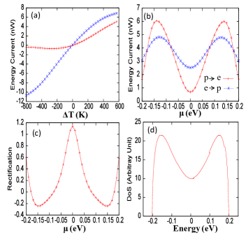
Figure 6: (a) The energy current with $\mu=0$ (red, solid) and $\mu=0.1$ eV (blue, dotted). We have set $T_{\rm e}=T+\Delta T/2$, $T_{\rm p}=T-\Delta T/2$, with $T=300$ K. (b) Fermi level ($\mu$) dependence of the energy current at fixed temperature difference $\Delta T=300$ K. (c) Rectification ratio $R$ as a function of $\mu$. (d) The electronic spectral function $A(\varepsilon)$ as a function of energy $\varepsilon$.

III.4 Effect of EPI on thermal transport in single-walled carbon nanotubes

Phonon modes can be excited by the mobile electrons due to the EPI effect; i.e., a high bias over the system leads to self-heating (Joule heating). In nanoscale electric devices, the electric current density can be much larger than that in the macroscopic system. The high current density will generate strong Joule heating, which may eventually break the device. In this sense, Joule heating becomes a bottleneck for further increase of the electric current density. Hence, lots of theoretical and experimental efforts have been devoted to understanding the Joule heating phenomenon in the nanoscale electric devices. In experiment, Joule heat can be measured via the thermal-mechanical expansion technique, which records the Joule heat induced temperature riseGrosse et al. (2013). The Joule heat can increase the temperature of the molecular junction from room temperature to 463 K, which has been examined through the inelastic electron tunneling spectroscopyTsutsui et al. (2008). Grosse et al. investigated the nanoscale Joule heating in phase change memory devicesGrosse et al. (2013). The Joule heating leads to the temperature rise in the phase change memory device, which results in an obvious volume expansion. In another experiment, Joule heating is found to be responsible for the correlated breakdown of nanotube forestsShekhar et al. (2011, 2012).

For a system without localized phonon modes, all phonon modes have important contribution to the Joule heat. The Joule heat contributed by these propagating phonon modes have important effects on the electric devices. For example, in graphene transistors, the output electric current will saturate with increasing source-drain voltageLiao et al. (2011); Islam et al. (2013). This saturated current density can be reduced by 16.5% due to the Joule heatingIslam et al. (2013).

The localized phonon modes exist around some defects or nonuniform configurations, such as the free edge, the isotropic doping, interface, etc. This particular type of phonon modes has no direct contribution to the thermal conduction, but localized phonon modes play a particularly important role in the Joule heat phenomenon. They are characteristic for their exponentially decaying vibration displacement; i.e., only a small portion of atoms are involved in the localized vibration. For instance, there are some localized edge phonon modes at graphene nanoribbon’s free edge. In these modes, edge atoms vibrate with large amplitude, but the vibrational displacement decays exponentially from the edge into the interior region.

The localized-phonon-mode-induced Joule heat was observed in graphene nanoribbons in experiment, and explained theoretically. Jia, et al. utilized Joule heating to trigger the edge reconstruction at the free edges in the graphene nanoribbonsJia et al. (2009). Engelund, et al. attributed this phenomenon to the Joule heating of the edge phonon modesEngelund et al. (2010). There are two conditions for the important Joule heating of the edge phonon modes. First, these localized edge phonon modes can spatially confine the energy at the edges. Second, the electrons interact strongly with the localized edge phonon modes. The mean steady-state occupation of the edge phonon mode can be calculated from the ratio of the current-induced phonon emission rate and damping rate. The effective temperature for the free edge can be extracted by assuming this occupation to be Bose distributed. The effective temperature was found to be as high as 2500 K for bias around 0.55 V. This high effective temperature was proposed to be the origin for the edge reconstruction.

Although Joule heating might be used for selectively bond-breakingKoch et al. (2006); Volkovich et al. (2011), its most common outcome is a disaster of device breakdown. The effective temperature is a suitable quantity to describe the Joule heating. In 1998, Todorov studied Joule heating problem in a molecular junctionTodorov (1998). In his work, the Einstein model is applied to represent the phonon modes in the system, and the electron-electron interaction is ignored as the system size is much smaller than the electron mean free path. Part of the EPI-induced Joule heat will be delivered out of the system by the phonon heat conduction, while the remaining Joule heat gives a high effective temperature. For low ambient temperature, the effective temperature scales with voltage $V$ as $T_{\rm eff}^{4}\approx\gamma^{4}V^{2}$, with $\gamma$ as an EPI-dependent constant. It was shown that the effective temperature can be above 200 K for a very low ambient temperature around 4 KAsai (2011). But at very high bias, the scaling law could differ from thisTsutsui et al. (2007).

There are several experimental approaches to investigate the effective temperature of the electric device induced by Joule heating. The effective temperature can be extracted by measuring some quantities that are temperature-dependent. For example, the breaking force of the single molecular junction is related to the temperature. This force-temperature relationship can be used to estimate the effective temperatureHuang et al. (2006). The Raman spectroscopy also depends on the temperature. Hence, it can be used to deduce the effective temperature of Raman-active phonon modesIoffe et al. (2008); Yu et al. (2011); Ward et al. (2011).

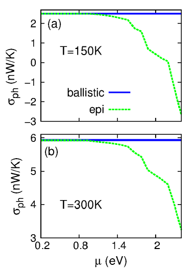
Figure 7: (Color online) The phonon thermal conductance versus chemical potential for metallic SWCNT (10, 10) at (a) 150 K and (b) 300 K. Solid line is for ballistic phonon thermal conductance without EPI effect. Reprinted from J. Appl. Phys., 110, 124319 (2011).

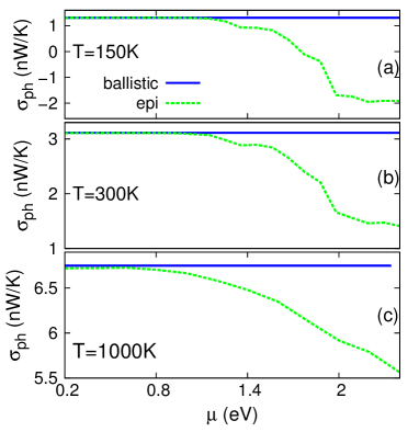
Figure 8: (Color online) The phonon thermal conductance versus chemical potential for semiconductor SWCNT (10, 0) at (a) 150 K, (b) 300 K, and (c) 1000 K. Solid line is for ballistic phonon thermal conductance without EPI effect. Reprinted from J. Appl. Phys., 110, 124319 (2011).

It has also been shown that EPI has an important effect on the thermal conductance in single-walled carbon nanotubes (SWCNTs)Jiang and Wang (2011). For them, we apply the Born approximation to consider the EPI effect using the NEGF approach, as the SCBA is computationally more expensive. The phonon thermal current can be calculated by considering the three EPI contributions shown in the Feynman diagrams in Fig. 2. The phonon thermal current flowing from the left lead into the center is given by Eq. (26). The expression for the right lead is analogous. The Joule heat is generated in the system and flows into the leads, so the total Joule heat is the sum of heat currents into both leads, $Q=-(I_{\rm p}^{L}+I_{\rm p}^{R})$. The thermal current from Eq. (26) also includes that induced by the temperature gradient, which satisfies $I_{\rm p}^{L}=-I_{\rm p}^{R}$. Hence, $Q$ gives solely the Joule heat.For metallic SWCNT (10, 10), both electrons and phonons are important heat carriers. The EPI only slightly reduces the electron thermal conductance, but it has a strong effect on the phonon thermal conductance. More specifically, Fig. 7 (a) shows an ‘electron-drag’ effect on the phonon thermal conductance at 150 K. The phonon thermal conductance becomes negative for high chemical potential value $\mu>2.0$ eV, which indicates that electrons can help to drag phonons from cold temperature region to the hot temperature region. The ‘electron-drag’ phenomenon happens at low temperature and high chemical potential, and it does not happen at a higher temperature 300 K as shown in Fig. 7 (b). For semiconductor SWCNT (10, 0), the electronic thermal conductance contributes less than 10% of the total thermal conductance at low bias (e.g. $\mu=0.3$ eV), while phonons make most significant contribution to the total thermal conductance. Similar ‘electron-drag’ phenomenon also exists in the semiconductor SWCNT (10, 0) at low temperature as shown in Fig. 8 (a).

IV Strong EPI regime: Quantum Master equation approach

IV.1 Quantum Master equation formulism

In this section, we introduce the QME approach to consider the case of strong EPI. Before doing that, we should mention that the NEGF method has also been used to treat the strong EPIFlensberg (2003); Galperin et al. (2004); Chen et al. (2005); Galperin et al. (2006); Sun and Xie (2007); Zazunov and Martin (2007). Since the idea behind it is very similar to that of the master equation approach, we choose not to introduce it here.

To simplify the formula, we ignore the coupling of molecular phonon modes to the phonon leads. The model Hamiltonian simplifies to

$$H_{\rm tot}=H_{S}+H_{\rm e}^{L}+H_{\rm e}^{R}+{V_{\rm e}}$$ (55)

where $H_{S}=H_{\rm p}^{C}+H_{\rm e}^{C}+H_{\rm ep}$ denotes the system Hamiltonian, and $V_{\rm e}=V_{\rm e}^{L}+V_{\rm e}^{R}$ is the system-lead coupling. In the QME formalism we assume the system-lead coupling $V_{\rm e}$ is weak so we can do perturbation on it. We work in the interaction picture with $H_{0}=H-V_{\rm e}$ as non-interacting part and $V_{\rm e}$ as the interaction. For simplicity, in this section we use $V$ to represent $V_{\rm e}$ since we don’t have $V_{\rm p}$. The equation of motion for the full density matrix follows the von Neumann equation

$$i\hbar\frac{\partial\rho_{I}(t)}{\partial t}=[V_{I}(t),\rho_{I}(t)].$$ (56)

Here, the subscript $I$ denotes operator in the interaction picture. The time argument in the parentheses means non-interacting evolution $O(t)=e^{iH_{0}t/\hbar}Oe^{-iH_{0}t/\hbar}$. The above equation can be written in an integral form as

$$\rho_{I}(t)=\frac{-i}{\hbar}\int_{t_{0}}^{t}\,dt^{\prime}[V_{I}(t^{\prime}),\rho_{I}(t^{\prime})]+\rho_{I}(t_{0}).$$ (57)

One can recursively apply the above equation to get a series expansion of the full density matrix in power of $V_{I}$. We truncate the series to the second order and differentiate it with respect to time $t$ at both sides of the equation to get the following integro-differential equation

$$\frac{\partial\rho_{I}(t)}{\partial t}{\approx}\frac{-i}{\hbar}[V_{I}(t),\rho_{I}(t_{0})]-\frac{1}{\hbar^{2}}\int_{t_{0}}^{t}dt^{\prime}[V_{I}(t),[V_{I}(t^{\prime}),\rho_{I}(t_{0})]].$$ (58)

We prepare the initial state as a product state of the system and each lead, $\rho(t_{0})=\tilde{\rho}(t_{0})\otimes\rho_{\rm e}^{L}\otimes\rho_{\rm e}^{R}$. For the system-lead coupling $V$ we assume it can be written as a product of system operator $S$ and lead operator $B$ as $V=\sum_{\alpha}S^{\alpha}\otimes B^{\alpha}$. In such cases we can trace over the lead degrees of freedom to get

$$\frac{\partial\tilde{\rho}_{I}(t)}{\partial t}=\frac{-1}{\hbar^{2}}\sum_{\alpha,\beta}\int_{t_{0}}^{t}\!\!dt^{\prime}[S_{I}^{\alpha}(t),S_{I}^{\beta}(t^{\prime})\tilde{\rho}_{I}(t_{0})]C^{\alpha\beta}(t-t^{\prime})+{\rm H.c.}$$ (59)

where $C^{\alpha\beta}(t-t^{\prime})=\mathrm{Tr}[\rho_{\rm e}^{L}\otimes\rho_{\rm e}^{R}B_{I}^{\alpha}(t)B_{I}^{\beta}(t^{\prime})]$ is the correlation function of the leads. Here we have used the condition that the expectation value of a single lead operator $B^{\alpha}$ is zero. We can now transform back to the Schrödinger  picture and extend the initial time $t_{0}$ to $-\infty$ to get the QME of Redfield typeRedfield (1965); Breuer and Petruccione (2007); Weiss (2008)

$$\frac{\partial\tilde{\rho}}{\partial t} = -\frac{{i}}{\hbar}[H_{S},\tilde{\rho}]-\frac{1}{\hbar^{2}}\sum_{\alpha,\beta}$$

$$\times\int_{-\infty}^{t}dt^{\prime}\bigl{\{}[S^{\alpha},S^{\beta}(t^{\prime}-t)\tilde{\rho}]C^{\alpha\beta}(t-t^{\prime})+{\rm H.c.}\bigr{\}}.$$

Here we have replaced $\tilde{\rho}(t_{0})$ by $\tilde{\rho}$, which is essential and correct only when one intends to get the 0th-order reduced density matrix $\tilde{\rho}^{0}$ by solving the above QMEThingna et al. (2014); Wang et al. (2014); Fleming and Cummings (2011). In the application to the EPI problem, by exact diagonalizing the system Hamiltonian, this Redfield QME can take into account the coherence between electrons and phonons, in contrast to the usual rate equation approachSegal and Nitzan (2005); Wu et al. (2009).

We write the above equation in the eigenbasis of the system Hamiltonian $H_{S}$ to obtainBreuer and Petruccione (2007); Zwanzig (2001)

$$\frac{d\tilde{\rho}_{nm}}{dt}=-\frac{{i}}{\hbar}\Delta_{nm}\tilde{\rho}_{nm}+\sum_{ij}R^{ij}_{nm}\tilde{\rho}_{ij},$$ (61)

where the relaxation tensor readsThingna et al. (2012)

$$R^{ij}_{nm} = \frac{1}{\hbar^{2}}\sum_{\alpha,\beta}\Bigl{\{}S^{\alpha}_{ni}S^{\beta}_{jm}W_{ni}^{\alpha\beta}$$ (62)

$$-\delta_{jm}\sum_{l}S^{\alpha}_{nl}S^{\beta}_{li}W_{li}^{\alpha\beta}\Bigr{\}}+\mathrm{H.c.}$$

The transition coefficients are given by

$$W_{kj}^{\alpha\beta}=\int_{-\infty}^{t}dt^{\prime}e^{{i}\Delta_{kj}(t^{\prime}-t)/\hbar}C^{\alpha\beta}(t-t^{\prime}),$$ (63)

where $\Delta_{kj}=E_{k}-E_{j}$ are the energy spacings of the system Hamiltonian.

Since we are only interested in the steady state, we impose the condition $d\tilde{\rho}/dt=0$ at $t=0$ and solve the above equation order by order with respect to $V$. One can find that all the off-diagonal elements of the 0th-order reduced density matrix vanish in steady state and the diagonal elements can be evaluated via the matrix equationThingna et al. (2012) $\sum_{i}R^{ii}_{nn}\tilde{\rho}^{(0)}_{ii}=0$, together with the constraint of $\mathrm{Tr}[\tilde{\rho}^{(0)}]=1$.

For the calculation of currents, we go through a similar derivation as the QME. The electronic current operator $\mathcal{J}_{\rm e}$ and heat current operator $\mathcal{J}_{\rm h}$ can be written in the form $\mathcal{J}_{\rm e(h)}=\sum_{\alpha}S^{\alpha}\otimes\mathcal{B}_{\rm e(h)}^{\alpha}$. The expectation value of currents can be calculated according to $I_{\rm e(h)}=\mbox{Tr}[\rho_{I}(t)\mathcal{J}_{I}(t)]$. Since we are interested in the lowest order of current, we truncate Eq. (57) to the lowest order and plug in to get

$$I_{\rm e(h)}=\frac{-i}{\hbar}\int_{t_{0}}^{t}\,dt^{\prime}\mbox{Tr}\bigl{\{}[V_{I}(t^{\prime}),\rho_{I}(t_{0})]\mathcal{J}_{I}(t)\bigr{\}}.$$ (64)

By taking the trace over the leads and transforming back to the Schrödinger  picture one obtains the current at $t=0$ as

$$I_{\rm e(h)} = \frac{1}{\hbar^{2}}\sum_{\alpha,\beta}\int_{-\infty}^{0}dt^{\prime}\mbox{Tr}[\tilde{\rho}S^{\alpha}S^{\beta}(t^{\prime})]\mathcal{C}_{\rm e(h)}^{\alpha\beta}(-t^{\prime})+\mathrm{H.c.},$$

where $\mathcal{C}_{\rm e(h)}^{\alpha\beta}(t)=\bigl{\langle}B^{\alpha}(t)\mathcal{B}_{\rm e(h)}^{\beta}(0)\bigr{\rangle}$ is the correlation function between the lead operators occurring in the system-lead coupling Hamiltonian and the current operator definition. For the same reason as the derivation of master equation, here $\tilde{\rho}(t_{0})$ needs to be replaced by $\tilde{\rho}$ to get correct steady state results. Since we are calculating lowest order of current, we can use the 0th order reduced density matrix $\tilde{\rho}^{(0)}$. Written in the eigenbasis of system Hamiltonian, the above equation becomes $I_{\rm e(h)}=\mathrm{Tr}\left[\tilde{\rho}^{(0)}\mathcal{I}^{r}_{\rm e(h)}\right]$ with the reduced current operator defined as

$$(\mathcal{I}^{r}_{\rm e(h)})_{ij}=\frac{1}{\hbar^{2}}\sum_{\alpha,\beta,k}\Bigl{[}S^{\alpha}_{ik}S^{\beta}_{kj}\mathcal{W}^{\alpha\beta}_{\rm e(h)}(\Delta_{kj})+{\rm c.c.}\Bigr{]},$$ (66)

where the transition coefficients are

$$\mathcal{W}_{\rm e(h)}^{\alpha\beta}(\Delta_{kj})=\int_{-\infty}^{0}d\tau e^{i\Delta_{kj}\tau/\hbar}\mathcal{C}_{\rm e(h)}^{\alpha\beta}(-\tau).$$ (67)

.

Up to now the QME formalism is general and not restricted to any specific form of system or leads Hamiltonians. For the application to transport problems with EPI as concerned in this review, the system-coupling Hamiltonian is considered as a tunneling HamiltonianMeir and Wingreen (1992). In such case the system operator $S$, leads operator $B$ and $\mathcal{B}$ can be specified as $S=\left\{d,d^{\dagger}\right\}$, $B=\left\{\sum_{k\in L,R}V_{k}c_{k}^{\dagger},\sum_{k\in L,R}V_{k}c_{k}\right\}$, $\mathcal{B}_{\rm e}=\left\{\,e\sum_{k\in L}V_{k}c_{k}^{\dagger},-e\sum_{k\in L}V_{k}c_{k}\,\right\}$ and $\mathcal{B}_{\rm h}=\left\{\,\sum_{k\in L}(\varepsilon_{k}-\mu_{L})V_{k}c_{k}^{\dagger},-\sum_{k\in L}(\varepsilon_{k}-\mu_{L})V_{k}c_{k}\,\right\}$. The infinite nature of the leads can be specified by defining a continuous spectra function for the leads

$$\Gamma_{\alpha}(\varepsilon) = -2{\rm Im}\Sigma_{\alpha}^{r}(\varepsilon)$$ (68)

$$= 2\pi\sum_{k\in\alpha}|V_{k}|^{2}\delta(\varepsilon-\varepsilon_{k}),\;\alpha=L,R.$$

Throughout this section we use a wide band spectra function for the electronic leads with Lorentzian cut-off as

$$\Gamma_{\alpha}(\varepsilon) = \frac{\eta_{\alpha}}{1+(\varepsilon/\varepsilon_{D})^{2}},\;\alpha=L,R.$$ (69)

The non-vanishing correlation functions can be evaluated via

$$C_{\alpha}^{12}(t) = \int_{-\infty}^{\infty}\frac{d\varepsilon}{2\pi}\Gamma_{\alpha}(\varepsilon)f_{\alpha}(\varepsilon)e^{\mathrm{i}\varepsilon t/\hbar},$$ (70)

$$C_{\alpha}^{21}(t) = \int_{-\infty}^{\infty}\frac{d\varepsilon}{2\pi}\Gamma_{\alpha}(\varepsilon)\bigl{(}1-f_{\alpha}(\varepsilon)\big{)}e^{-\mathrm{i}\varepsilon t/\hbar}\!\!,$$ (71)

$$\mathcal{C}_{\rm h}^{12}(t) = \int_{-\infty}^{\infty}\frac{d\varepsilon}{2\pi}(\varepsilon-\mu_{L})\Gamma_{L}(\varepsilon)f_{L}(\varepsilon)e^{\mathrm{i}\varepsilon t/\hbar},$$ (72)

$$\mathcal{C}_{\rm h}^{21}(t) = \int_{-\infty}^{\infty}\frac{d\varepsilon}{2\pi}(\varepsilon-\mu_{L})\Gamma_{L}(\varepsilon)\bigl{(}1-f_{L}(\varepsilon)\big{)}e^{-\mathrm{i}\varepsilon t/\hbar},$$

and $C^{12}(t)=C^{12}_{L}(t)+C^{12}_{R}(t)$, $\mathcal{C}_{\rm e}^{12}(t)=-eC_{L}^{12}(t)$, $\mathcal{C}_{\rm e}^{21}(t)=eC_{L}^{21}(t)$. We note that here the upper index $1$ or $2$ refers to the two components of $B$ and $\mathcal{B}_{\rm e/h}$ given above. For the system Hamiltonian, we focus only on the single electronic level coupled to a single phonon mode representing the center of mass of the molecule. In such case, the system Hamiltonian will reduce to

$$H_{S}=\varepsilon_{0}d^{\dagger}d+\hbar\omega_{0}a^{\dagger}a+\lambda d^{\dagger}d(a^{\dagger}+a)$$ (74)

with $\omega_{0}$ the angular frequency of the phonon mode and $\lambda$ denotes the EPI strength. This type of Hamiltonian has been well-studied in the context of molecular junctionChen et al. (2005); Koch and von Oppen (2005); Sun and Xie (2007); Lü and Wang (2007); McEniry et al. (2008); Asai (2008); Lee et al. (2009); Leijnse et al. (2010); Zianni (2010); Piovano et al. (2011); Koch et al. (2011); Zhou and Li (2012); Arrachea et al. (2014); Koch et al. (2014); Perroni et al. (2014).

The QME formalism treats the nonlinearity of EPI exactly. Therefore in this section we will focus on strong EPI regime with emphasis on the EPI strength dependence of the electron/heat current. In the following we will discuss the effect of EPI on the electronic transport properties, including the phonon sidebands, negative differential resistance, thermoelectric properties and local heating effects.

IV.2 Phonon sidebands and negative differential resistance

One of the earliest findings of the vibrational effects on the electronic transport through a molecular quantum dot is the appearance of the phonon sidebands in the $I-V$ characteristics. When electrons transport through a single electronic level, the differential conductance ($dI/dV$) will manifest a peak at resonant level when plotted against the voltage bias ($V$). However, when the electronic level is interacting with a vibrational mode, replica side peaks will appear at the side of the resonant peaks. These side peaks are called phonon sidebands. A simple reason for the appearance of phonon sidebands is due to the fact that the electrons can emit or absorb phonons when they pass through the molecule. Therefore, the distance between each adjacent peaks is always equal to a single phonon energy. The phonon sidebands attract wide attentions in molecular junction systems. Experimentally, phonon sidebands were found in 1980sGoldman et al. (1987) and then were utilized to identify vibrational modes in molecular junctions Park et al. (2000, 2002); Zhitenev et al. (2002); Yu and Natelson (2004) and quantum wiresAgraït et al. (2002a, b); de la Vega et al. (2006); Paulsson et al. (2005); Viljas et al. (2005). Theoretically, at the beginning the sidebands were investigated by using scattering theory, which gives the transmission probability $T({\varepsilon,\varepsilon^{\prime}})$ for an electron to passing through an EPI system. The electron is coming from vacuum at energy ${\varepsilon}$ and leaving at energy ${\varepsilon^{\prime}}$Wingreen et al. (1988). The scattering theory predicts side peaks in the transmission probability, which qualitatively justifies the phonon sidebands in molecular junction systems. However, prediction of phonon sidebands in the lead-molecule-lead junctions is a much more difficult task. A simple generalization to take the Fermi-Dirac statistics nature of the electron leads into account is to weight the exact transmission probability with the Fermi-Dirac distribution of each lead, i.e., by multiplying the transmission probability $T({\varepsilon,\varepsilon^{\prime}})$ by a factor $f_{L}({\varepsilon})[1-f_{R}({\varepsilon^{\prime}})]$ as a new transmission probability for electron going from the left lead to the right lead through the nano-conductor. This approximation is called single particle approximation (SPA). Plenty of earlier work is in this framework and it predicts Lorentzian type of phonon sidebands with the same width. But obviously this method assumes each electron transports independently through the junction, where the many-body effects are ignored. As a result, it overestimates the currents and it is not able to predict the quantized conductance $e^{2}/h$ either.

Based on the NEGF technique, more rigorous methods merged in dealing with the nonlinearity in EPI, such as the Green’s function equation of motion method (EOM) Flensberg (2003), SCBAMitra et al. (2004); Chen et al. (2005); Galperin et al. (2006, 2004) and nearest neighbor crossing approximation (NNCA)Zazunov and Martin (2007). All of the above are Green’s function based formalisms with different kinds of approximations. In general these approaches predict that the phonon side peaks are much sharper than the SPA approach. This sharpness is closely related to the Pauli exclusion, which the SPA approach failed to take into account. Other than Green’s function based methods, another approach is to use rate equation of electron occupation probability in the molecule, via calculating the transition coefficients of the electron to tunnel from the molecule to each lead and vice versa. This method assumes the transport is an electron tunneling process and the electron will lose its phase information when it resides in the molecule. Therefore it will be valid when the molecule-lead coupling is weak and the coherence of the electron and phonon in the molecule can be neglected. For all these formalisms, we would like to point out that one should take care of the phonon distribution. Treating the phonon at equilibrium distribution at a fixed temperature could be valid when the EPI strength is much weaker than the coupling strength between the phonon and its environment. However, when the environmental influence is weak, one should consider phonons in nonequilibrium states. This nonequilibrium treatment of phonon distribution can have pronounced effect on $I-V$ characteristics due to the fact that the current induced vibrational excitation can be significantMitra et al. (2004); Härtle and Thoss (2011).

Besides the peak distances and peak width discussed above, other aspects characterizing the sidebands include the weights of the zero-phonon band and the number of peaks. The investigation of these properties mainly focuses on the effects of EPI strength, Fermi energy of the molecule, chemical potential and temperature of the leads. In general, the higher order peaks will be suppressed by the Frank-Condon factor Entin-Wohlman et al. (2009); Härtle and Thoss (2011); Monreal et al. (2010). In the framework of NEGF, Chen $et$ $al$. found that the weight from zero-phonon band will decrease monotonically with increase of EPI strength and temperature while the weights of higher order sidebands will increase and then decrease Chen et al. (2005). The chemical potentials of the leads will influence the presence of the sidebands at both sides of the zero phonon peaks [Fig. 9, panel (a) and (b)]. If one keeps the chemical potential of one lead fixed and increases the chemical potential of the other lead, the phonon sidebands will appear only at one side of the 0-th order peak [Fig 9, panel (c)]. However, if one fixes the Fermi-level of the molecule and changes the chemical potentials of both leads, phonon sidebands will appear at both sidesGalperin et al. (2006); Chen et al. (2005). We note that, in this section, Fermi-level of the molecule is defined as $(\mu_{L}+\mu_{R})/2$.

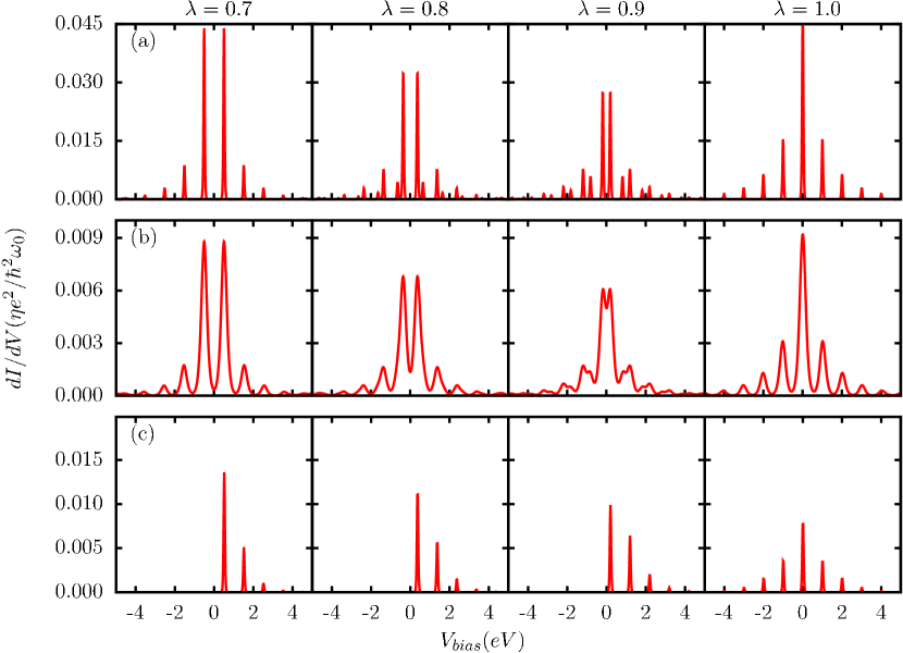
Figure 9: The phonon sidebands with different EPI strength with (a) low temperature ($T=0.02\hbar\omega_{0}/k_{B}$) and symmetrically biased voltage ($V_{L/R}=\pm V_{bias}$), (b) high temperature ($T=0.1\hbar\omega_{0}/k_{B}$) and symmetrically biased voltage, (c) low temperature and asymmetric biased voltage ($V_{L}=V_{bias}$ and $V_{R}=0$). Other parameters include $\varepsilon_{0}=1.0\hbar\omega_{0}$, $\varepsilon_{D}=10\hbar\omega_{0}$ for all plots.

In the framework of QME formalism described earlier, which is exact in the weak system-lead coupling limit, we find phonon sidebands for the single electronic level interacting with a single phonon mode. In this case the zero-phonon peak will occur at the renormalized resonant level due to polaron shift ($\varepsilon_{0}-\lambda^{2}/\hbar\omega_{0}$) and the sidebands will appear at every distance of $\hbar\omega_{0}$. The peaks will appear at each side of zero-phonon peak under symmetric change of the lead chemical potentials while only appear at one side if we fix chemical potential of one lead. The EPI strength will not only shift the peaks, but also modulate the weights of the peaks. We find that upon increasing either EPI strength or temperature, the weight of the zero-phonon peak will decrease, which is consistent with the previous workChen et al. (2005). However, interesting phenomena happen when the renormalized level of the quantum dot gets close to the Fermi-level of the dot, [$\varepsilon_{0}-\lambda^{2}/\omega_{0}\approx(\mu_{L}+\mu_{R})/2$], i.e., additional peaks appear at each side. Those peaks have distance $\hbar\omega_{0}$ with the zero-order peak at the opposite side. However, the two major peaks really merge together, and those additional peaks disappear again. In the case of asymmetric change of lead chemical potential (right most panel of Fig. 9 (c)), we found peaks appear at both sides when the zero-phonon peaks merge together.

Another interesting perspective of the $I-V$ characteristics is the phenomenon of the negative differential resistance (NDR), where the current decreases with the increase of voltage bias. The NEGF formalism predicts that NDR is impossible in ballistic electronic transport, but it will emerge in the presence of EPI. NDR has been both theoretically investigatedZazunov et al. (2006); Härtle and Thoss (2011); Egger and Gogolin (2008) and experimentally measuredLeRoy et al. (2004). An important reason of NDR is due to the redistribution of the molecular states. As discussed in the previous section, the zero-phonon band carries major portion of electronic current. The probability for the molecule to be in that state will be related to the chemical potential of the leads. If one increases the bias via increasing the chemical potential of one lead, one actually lifts the Fermi-level of the molecule as well. If one brings the Fermi-level of molecule far away from the eigenenergy of zero phonon state, the probability of the molecule to be in that state will decrease and thus the current will decrease. Based on this analysis one can draw several immediate conclusions: 1. If one increases the bias simultaneously for both leads in pace and keeps the Fermi-level of the molecule fixed, there will be no NDR. 2. If one treats the phonon fixed in the equilibrium distribution, NDR will not appearHärtle and Thoss (2011). 3. If the chemical-potential-varying lead couples stronger to the molecule than the chemical-potential-fixed lead, the redistribution will be more sensitive, thus the NDR will be enhanced.

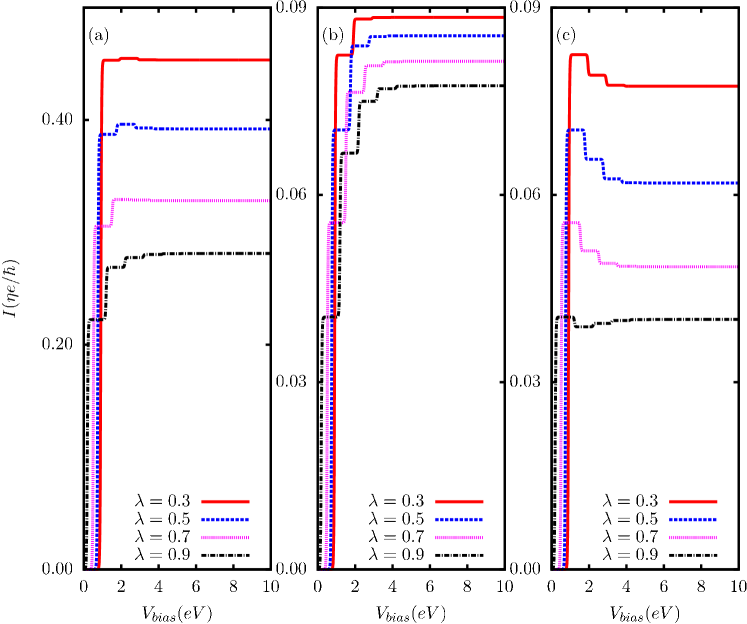
Figure 10: Prediction of NDR using QME formalism with the coupling strength (a) $\eta_{L}=0.1\eta_{R}$, (b) $\eta_{L}=\eta_{R}$ and (c) $\eta_{R}=0.1\eta_{L}$. For all plots $V_{R}$ is fixed at 0 and $V_{L}=V_{bias}$. The temperature is fixed at $T=0.02\hbar\omega_{0}/k_{B}$ for all leads. Other parameters are the same as Fig. 9

Figure 10 shows the NDR predicted in the QME formalism. We find that the NDR appears in the symmetric system-lead coupling. Moreover, NDR will be enhanced if the chemical-potential-varying lead couples stronger to the molecule than the other lead, but it will disappear in the other way around. We also find that NDR is most pronounced in the moderate EPI regime, while it is less significant in both weak and strong EPI regimesHärtle and Thoss (2011).

IV.3 Vibrational effect on thermoelectricity

In this part, we study the effects of EPI on the thermoelectric properties of the nano-conductor. We first look at the thermoelectric current, which is the electronic current induced by a temperature difference between the leads. Thermoelectric current exhibits quite different features comparing with voltage-bias current. It will increase monotonically and smoothly with the increasing of the temperature bias. Therefore, there will be no phonon sidebands. This is expected, because under temperature bias, the tunneling channel of the electron is always restricted to the molecular state that is close to the chemical potential of the leads. The increasing of temperature will only excite more conducting electrons, but not be able to extend extra tunneling channels. Therefore, there will be no sudden change of thermoelectric current. Due to the same reason, there will be no NDR effect as the increasing of the temperature bias will always make more electrons to be involved in tunneling. The restriction on tunneling channels also makes the thermoelectric current much smaller than the voltage-bias current.

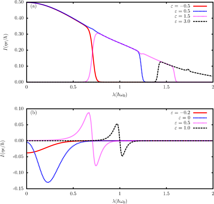
Figure 11: The dependence of voltage-bias current (a) and thermoelectric current (b) on the EPI strength under different $\varepsilon_{0}$. For panel (a), $\mu_{L}=\hbar\omega_{0}$, $\mu_{R}=-\hbar\omega_{0}$ and $T^{L}=T^{R}=0.02\hbar\omega_{0}$. For panel (b), $T^{L}=0.08\hbar\omega_{0}$, $T^{R}=0.02\hbar\omega_{0}$ and $\mu_{L}=\mu_{R}=0$.

The dependence of electronic conductance on the chemical potentials of the leads has been discussed in the Subsec. III.2. The sign of the Seebeck coefficient indicates that the currents will change direction with different chemical potential. Another interesting perspective is to find the dependence of currents on EPI strength. Figure 11 shows the plot of voltage-bias current [panel (a)] and thermoelectric current [panel (b)] with the EPI strength $\lambda$. For voltage-bias current, we find that the current decays with EPI strength in general. More precisely, the maximum current one can achieve via adjusting the $\varepsilon_{0}$ is decreasing monotonically with EPI strength. This is due to the Frank-Condon blockage of the current. However, for each $\varepsilon_{0}$ we can find the enhancement of current due to EPI, and that is mainly because of the polaron shift which can bring the electron resonance level into the conduction band from outside. For the thermoelectric current, the profile is quite different. We see that the current can change sign with the increase of EPI strength when $\varepsilon_{0}$ is higher than the Fermi level, which indicates that the EPI can switch the charge carriers of the quantum dot between electrons and holesZhou et al. (2015). For each $\varepsilon_{0}$ there exist two optimized values of EPI strength such that the thermoelectric current maximizes. This optimized $\lambda$ shifts left with decrease of $\varepsilon_{0}$ until disappear one by one at the $\lambda=0$ end.

One important quantity to describe the efficiency of the thermoelectric material is the figure of merits $Z_{\rm e}T$. It is related to the electronic conductance $G_{\rm e}$, Seebeck coefficient $S$, thermal conductance $G_{h}$ via the formula $Z_{e}T=G_{\rm e}S^{2}T/G_{h}$. Here we use the notation $Z_{\rm e}T$ to denote the figure of merits of the system by ignoring the thermal conductance due to phonons. So $G_{h}$ here only takes account the thermal conductance due to electrons. The effect of phonons on the figure of merit $Z_{e}T$ is rather complicated, which is closely related to the electron Fermi energyKoch et al. (2014); Perroni et al. (2014); Leijnse et al. (2010); Ren et al. (2012), the phonon energy Zianni (2010), the temperature and chemical potentials of the leadsKoch et al. (2014); Perroni et al. (2014); Ren et al. (2012); Hsu et al. (2012). Figure 12 shows the dependence of the electronic conductance, thermal conductance, Seebeck coefficient and figure of merit on the electron energy $\varepsilon_{0}$ and EPI strength $\lambda$. The major effect of EPI is on the thermal conductance of the molecular junctionZianni (2010). The EPI can open extra channels, from which high energy electrons can tunnel from hotter lead to colder lead, while low energy electrons tunnel in the opposite direction. Therefore, the thermal conductance is enhanced while the electronic conductance is not affected too much. Due to the increase of the thermal conductance, $Z_{e}T$ will be suppressed drasticallyZianni (2010); Perroni et al. (2014). Though the figure of merits $Z_{e}T$ will be reduced quickly under the influence of phonon scattering in weak EPI regime, it will gradually saturate at strong EPI regime. We also would like to point out that when the electron energy is close to the Fermi energy of the quantum dot, the Seebeck coefficient and hence the $Z_{e}T$ will become very small. However, the phonon scattering can renormalized the electron energy via polaron shift and thus the Seebeck coefficient can be enhanced. As a result, EPI can enhance $Z_{e}T$ in this particular parameter regime.

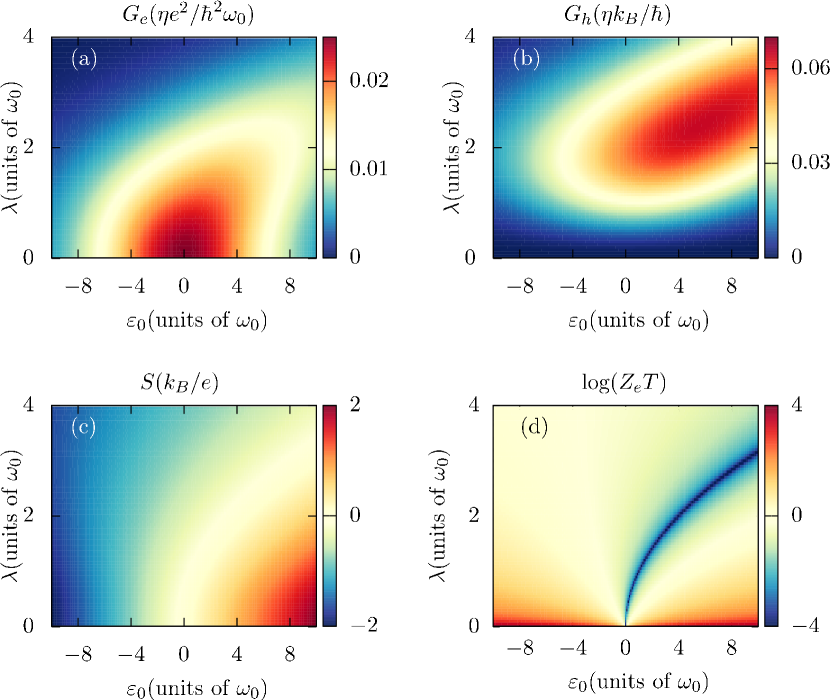
Figure 12: The contour plot of electronic conductance $G_{\rm e}$, thermal conductance $G_{h}$, Seebeck coefficient $S$ and figure of merit $Z_{e}T$ with respect to $\varepsilon_{0}$ and $\lambda$. The parameters are: $\mu=0$, $T=5\hbar\omega_{0}/k_{B}$. For this plot, the phonon mode is coupled to its environments at temperature $T$ with coupling strength $\eta_{E}=0.1\eta$. Figure adapted with permission from Phys. Rev. B, 91, 045410 (2015). Copyrighted by the American Physical Society.

IV.4 Local heating

Local heating is an important phenomenon in molecular junction, not only due to its own importance affecting the stability of the system, but also due to its close relation to the phonon sidebandsMitra et al. (2004), NDR and thermoelectric effectHsu et al. (2012, 2010). The distribution of the phonon states in current-carrying system can be far away from equilibriumMitra et al. (2004), or in some cases, may even lead to phonon instabilityLü et al. (2010, 2011a); Härtle and Thoss (2011); Simine and Segal (2012). Phonons can be excited significantly by the voltage biasHärtle and Thoss (2011), and in turn affect the $I-V$ characteristics. At each peak of the phonon sidebands, one can actually find a vibrational excitation eventGalperin et al. (2007b); Härtle and Thoss (2011). Previous study also found that the local heating can enhance the thermoelectric efficiencyHsu et al. (2010, 2012). However, in most cases local heating is not preferred because it will affect the stability of the systemJiang and Wang (2011) and introduce noise to the measurementsBlanter et al. (2004); Clerk and Bennett (2005); Mozyrsky et al. (2004); Zippilli et al. (2010). Therefore, lot of effort has been put into cooling the system using electronic current, such as using superconducting single electron transistorNaik et al. (2006), or double quantum dotsZippilli et al. (2010).

Here we study the effects of the electronic current on the phonon mode of the nano-conductor. To investigate the local heating, effective temperatures are usually defined in various waysDubi and Di Ventra (2011); Galperin et al. (2007a); Lü and Wang (2007); Dubi and Di Ventra (2009); Jacquet and Pillet (2012); Bergfield et al. (2013). In this part, since we only have one single phonon mode, instead of defining the effective temperature, we use average phonon number to characterize the local heating effect. The way to specify the electronic current induced heating is to compare the nonequilibrium phonon number $n_{\rm neq}$ with equilibrium phonon number $n_{\rm eq}$. When the molecule is weakly coupled to the leads, the molecular states statistics will follow canonical distribution $\tilde{\rho}=e^{-\beta H_{S}}/\mathrm{Tr}(e^{-\beta H_{S}})$ and thus the equilibrium phonon number can be calculated exactly as Zhou et al. (2015)

$$n_{\rm eq}=\frac{1}{e^{\beta\hbar\omega_{0}}-1}+\frac{\lambda^{2}/(\hbar\omega_{0})^{2}}{e^{\beta(\varepsilon_{0}-\lambda^{2}/(\hbar\omega_{0}))}+1}.$$ (75)

The first term is the Bose-Einstein distribution function, the second term is a correction due to the polaron energy shift. The nonequilibrium phonon number can be calculated from the nonequilibrium reduced density matrix obtained from the QME. Figure 13 shows the difference of phonon numbers under voltage bias (top) and temperature bias (down). For voltage bias, $\Delta n$ is always positive which indicates that the system is always heated up. The yellow regime where $\Delta n\approx 0$ is the regime where the electronic current vanishes. When there is electronic current passing through, the heating effect is generally more pronounced in stronger EPI regime. However, for the temperature bias, we find both heating ($\Delta n>0$) and cooling regimes ($\Delta n<0$). Therefore, the local heating effect is not only related to the magnitude of electronic current, but also related to the energy each electron carries when it tunnels into the molecule. For the thermoelectric current, low energy electron can tunnel from the cooler lead to the molecule, absorb a phonon and tunnel to the hotter lead, resulting in cooling of the molecule. Such process is impossible in the voltage-bias case in the present setup as the electron is always flowing from the higher chemical potential side to the lower chemical potential side.

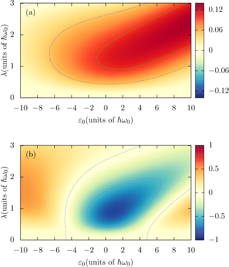
Figure 13: The correction of phonon number due to electronic current under voltage bias (a) and temperature bias (b). The parameters are: $\mu_{L}=-\mu_{R}=2\hbar\omega_{0}$, $T^{L}=T+\Delta T$, $T^{R}=T-\Delta T$, $\Delta T=3\hbar\omega_{0}/k_{B}$ and $T=5\hbar\omega_{0}/k_{B}$. The phonon is weakly coupled to its own environment at temperature $T$. Figure adapted with permission from Phys. Rev. B, 91, 045410 (2015). Copyrighted by the American Physical Society.

V Current-induced semi-classical Langevin dynamics

In the previous two sections, we mainly look at the effect of phonons on the electric and thermoelectric transport properties of electrons, which is also the focus of most published work. But, to study the current-induced forces, and their effect on atomic dynamics, we need to turn around. In this section, starting from the total Hamiltonian $H_{\rm tot}$, we derive a semi-classical Langevin equation to describe the atomic dynamics of the system, coupled to both phonon and (nonequilibrium) electron leads. The Langevin equation applies to the weak EPI regime, since similar to Sec. III our expansion parameter is the interaction matrix $M$. However, the derivation is not limited to the form of $H_{\rm tot}$. Following the same procedure we discuss below, we can also do an adiabatic expansion of the electron influence functional over the velocity of the ions. In that case, the Langevin equation applies to slow ions, but the EPI could be of arbitrary magnitudeLü et al. (2010, 2012); Bode et al. (2011, 2012).

The advantage of the Langevin equation approach is that, we can easily include the anharmonic phonon interaction, as in other molecular dynamics method. The anharmonic interaction is crucial in dealing with current-induced dynamics. This is because the phonon modes that interact with electrons are normally high-frequency ones, while the low frequency modes conduct heat from the system to surrounding electrodes more effectively. The energy transfer from high to low frequency modes is possible only when anharmonic interaction is included. Although possible, it is not a trivial task to incorporate anharmonic interactions in the NEGF or QME approach.

V.1 Initial states and reduced density matrices

We assume at a remote past $t_{0}$ and earlier time, the central system is decoupled with the leads and there is also no EPI, so that the electrons and phonons are also decoupled. The density matrix is assumed to be product of known equilibrium states. For example, the left lead is specified by

$$\rho^{L}_{\rm e} \propto e^{-\beta_{L}(H^{L}_{\rm e}-\mu_{L}N^{L})},$$ (76)

$$\rho^{L}_{\rm p} \propto e^{-\beta_{L}H_{\rm p}^{L}}.$$ (77)

Exactly what to take for the center is not important as for steady state with $t_{0}\to-\infty$, the results do not depend on it (except maybe in very subtle cases).

The density matrix (of the whole system) is governed by the von Neumann equation, and formally we can write

$$\rho(t)=U(t,t_{0})\rho(t_{0})U(t_{0},t),$$ (78)

where

$$U(t,t_{0})=Te^{-(i/\hbar)\int_{t_{0}}^{t}H_{\rm tot}(t^{\prime})dt^{\prime}}$$ (79)

assuming $t>t_{0}$. For the other case of $t<t_{0}$, the time-order operator $T$ should be replaced by the anti-time order operator. We are interested only in the center, so the leads degrees of freedom will be traced out. For notational simplicity, we assume only one left lead. The result for two or more leads is trivially generalized. We define

$$\tilde{\rho}(t) = {\rm Tr}_{L}\rho(t),$$ (80)

$$\tilde{\rho}_{{\rm p}}(t) = {\rm Tr}_{{\rm e}}\tilde{\rho}(t),$$ (81)

where the first reduced density matrix only eliminates the lead, while the last one eliminates the electrons as well, leaving only an effective density matrix for the phonons. The procedure to eliminate the lead for both the electrons and phonons follows the standard method of Feynman and Vernon Feynman and Vernon (1963), except that we need to be careful for the electrons which are fermions. Since there is no coupling between electrons and phonons in the leads, the phonon and electron degrees of freedom can be done separately (the initial density matrix is a product of the two).

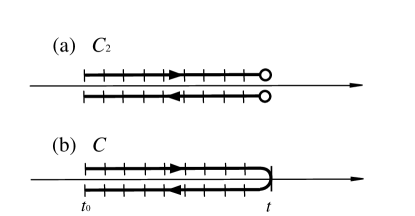
Figure 14: Two types of paths in the Feynman-path integrals. (a) two-segment path $C_{2}$. (b) Keldysh type closed contour $C$. The ticks represent the discretized integration variables; the open circles are not integrated.

V.2 Influence functional for phonons

The matrix elements of the density operator $\rho(t)$ is taken in the basis of the coordinates $u$. Following the standard treatment Kleinert (2009); Weiss (2008), the density matrix is then given by

$$\langle u^{\prime}|\rho(t)|u\rangle\propto\int\mathcal{D}[u]e^{(i/\hbar)\int_{C_{2}}\mathcal{L}(u,\dot{u})d\tau}\rho_{0}(u^{\prime}_{0},u_{0}).$$ (82)

The path $C_{2}$ consists of two segments (see Fig. 14(a)) running from time $t$ with coordinate variable $u$ back to $t_{0}$ at variable $u_{0}$, and then second segment running from $t_{0}$ with variable $u^{\prime}_{0}$ forward to time $t$ with variable $u^{\prime}$. Since the arbitrary constant in the proportionality can be fixed by normalization (${\rm Tr}\rho=1$), we need not specify precisely the measure associated with $\mathcal{D}[u]$. The path integral integrates all the intermediate variables except the two open ends at time $t$.

To eliminate the lead, the phonon Lagrangian is split into $\mathcal{L}=\mathcal{L}^{C}+\mathcal{L}^{L}-V$ where $V$ is the coupling potential energy term between the lead and center, given by $V=(u^{C})^{T}V^{CL}u^{L}$. The integration volume elements are also split $\mathcal{D}[u]=\mathcal{D}[u^{C}]\mathcal{D}[u^{L}]$. The initial distribution is assumed product type $\rho_{0}^{L}\otimes\rho_{0}^{C}$. Taking the trace of Eq. (82) means that we identify $u^{L}$ and $(u^{\prime})^{L}$ as the same variable $u^{L}$ and integrate it out. As far as variable $u^{L}$ is concerned, the path is of Keldysh type, i.e., running from $t_{0}$ to $t$ from above and then back from $t$ to $t_{0}$, as shown in Fig. 14(b). The reduced density matrix is then

$$\tilde{\rho}(t)=\int\mathcal{D}[u^{C}]e^{(i/\hbar)\int_{C_{2}}\mathcal{L}^{C}d\tau}I[u^{C}(\tau)]\rho_{0}^{C}((u^{\prime})_{0}^{C},u_{0}^{C}),$$ (83)

with the influence functional

$$I[u^{C}(\tau)]=\int\mathcal{D}[u^{L}]\rho_{0}^{L}((u^{\prime})_{0}^{L},u_{0}^{L})e^{(i/\hbar)\int_{C}(\mathcal{L}^{L}-V)d\tau}.$$ (84)

The above expression can be further simplified. Firstly, the initial distribution of the lead is in thermal equilibrium, $\rho_{0}^{L}\propto e^{-\beta_{L}H_{L}}$. Secondly, we can rewrite the path integral formula back into the operator form; thus, we obtain

$$I[u^{C}(\tau)] = {\rm Tr}\left[\frac{e^{-\beta_{L}H^{L}}}{Z_{L}}T_{C}e^{-(i/\hbar)\int_{C}(H^{L}+V)d\tau}\right]$$ (85)

$$= \langle T_{C}e^{-(i/\hbar)\int_{C}(H^{L}+V)d\tau}\rangle_{{\rm eq.L}},$$

where $Z_{L}$ is the canonical partition function, $T_{C}$ is contour order operator, the subscript eq.L stands for equilibrium average with respect to the left lead. One more transformation can be made to simplify it further. The time-dependence (or rather, contour time $\tau$ dependence) is understood to be in the Heisenberg picture governed by the Hamiltonian $H^{L}+V(\tau)$ which is different in the forward and backward direction. We can work in the interaction picture, thus eliminate the explicit $H^{L}$ from the formula. The resulting equation is

$$I[u^{C}(t)]=\langle T_{C}e^{-(i/\hbar)\int_{C}V_{I}(\tau)d\tau}\rangle_{{\rm eq.L}}.$$ (86)

This is the same equation [Eq. (5)] given in Ref. Stockburger and Grabert, 2002.

The influence functional can be calculated explicitly since the interaction $V$ is a quadratic form, and the contour operator naturally leads to contour ordered Green’s functions and Wick’s theorem is valid. We define the contour ordered phonon Green’s function of the lead as

$$d_{L}(\tau,\tau^{\prime})\equiv-\frac{i}{\hbar}\langle T_{C}u^{L}(\tau)u^{L}(\tau^{\prime})^{T}\rangle_{{\rm eq.L}}.$$ (87)

Expanding the exponential (or a cumulant expansion, expanding and taking logarithm), we get

$$I[u^{C}(t)]=\bigl{\langle}T_{C}\bigl{(}1-\frac{i}{\hbar}\int_{C}V_{I}(\tau)d\tau-\frac{1}{2\hbar^{2}}\int_{C}d\tau\int_{C}d\tau^{\prime}V_{I}(\tau)V_{I}(\tau^{\prime})+\cdots\bigr{)}\bigr{\rangle}$$ (88)

$$= T_{C}\bigl{(}1-\frac{1}{2\hbar^{2}}\int_{C}\int_{C}u^{C}(\tau)^{T}V^{CL}\langle T_{C}u^{L}(\tau)u^{L}(\tau^{\prime})^{T}\rangle V^{LC}u^{C}(\tau^{\prime})d\tau d\tau^{\prime}+\cdots\bigr{)}$$

$$= T_{C}\bigl{(}1-\frac{i}{\hbar}\frac{1}{2}\int_{C}d\tau\int_{C}d\tau^{\prime}u^{C}(\tau)^{T}\Pi_{L}(\tau,\tau^{\prime})u^{C}(\tau^{\prime})+\cdots\bigr{)}\qquad\qquad\qquad\qquad$$

$$= e^{-\frac{i}{\hbar}\frac{1}{2}\int_{C}d\tau\int_{C}d\tau^{\prime}u^{C}(\tau)^{T}\Pi_{L}(\tau,\tau^{\prime})u^{C}(\tau^{\prime})}.\qquad\qquad\qquad\qquad$$

The first order term (and all odd order in $V$ terms) vanishes, because $\langle u^{L}\rangle=0$. We have defined the ubiquitous contour ordered self-energy due to the lead as

$$\Pi_{L}(\tau,\tau^{\prime})=V^{CL}d_{L}(\tau,\tau^{\prime})V^{LC}.$$ (89)

It can be shown that the last line in the above derivation is an exact result.

It is instructive to clarify and compare with other notations used in the literature. A commonly used notation is (e.g., Ref. Weiss, 2008)

$$\ln I = -\frac{1}{\hbar}\int_{t_{0}}^{t}dt_{1}\int_{t_{0}}^{t_{1}}dt_{2}\left(u^{+}(t_{1})-u^{-}(t_{1})\right)^{T}$$ (90)

$$\times\left[L(t_{1},t_{2})u^{+}(t_{2})-L^{*}(t_{1},t_{2})u^{-}(t_{2})\right].$$

Using the rules $\int_{C}d\tau\to\sum_{\sigma}\int_{t_{0}}^{t}\sigma dt$, and $\Pi(\tau,\tau^{\prime})\to\Pi^{\sigma,\sigma^{\prime}}(t,t^{\prime})$, $u^{C}(\tau)\to u^{\sigma}(t)$ where $\sigma=+$ or $-$ for the upper and lower branch, the relations among the various self-energies, and symmetry relation $\Pi_{ij}^{>}(t,t^{\prime})=\Pi_{ji}^{<}(t^{\prime},t)$, we can rewrite Eq. (88) in the form of Eq. (90). By comparison, we find

$$L(t,t^{\prime})=i\Pi^{>}_{L}(t,t^{\prime}),\quad L^{*}(t,t^{\prime})=i\Pi^{<}_{L}(t,t^{\prime}).\quad$$ (91)

$\alpha(t,t^{\prime})\equiv L(t,t^{\prime})$ is the notation used by Schmid Schmid (1982).

V.3 Influence functional for electrons

The derivation of the influence functional for the electrons is similar except that we have to deal with grassmann integralsHedegård ; Chang and Chakravarty (1985); Hedegård and Caldeira (1987); Chen (1987). We follow the approach of Weinberg Weinberg (2005). To do the trace over the leads we need a specific representations for the operator $\rho$. For the electrons, we use the coherent state characterized by grassmann numbers such that

$$\hat{c}_{i}|c\rangle=c_{i}|c\rangle.$$ (92)

The hat denotes operator, without hat, it is a grassmann number. The state $|c\rangle$ has explicit form given as

$$|c\rangle \equiv e^{\sum_{i}\hat{c}_{i}^{\dagger}c_{i}}|0\rangle,$$ (93)

$$\langle c| \equiv \langle 0|\prod_{i}\hat{c}_{i}e^{\sum_{i}c_{i}\hat{c}_{i}^{\dagger}}.$$ (94)

The orthogonality is in the form

$$\langle c^{\prime}|c\rangle=\prod_{i}(c_{i}-c^{\prime}_{i}).$$ (95)

Similar states for the creation operator $\hat{c}_{j}^{\dagger}$ can be constructed with eigenvalue (a grassmann number) $\tilde{c}$, given the following results (similar to inner product of eigen states of $u$ and its conjugate momentum $p$ and completeness of the eigenstates).

$$\langle c|\tilde{c}\rangle = \cdots e^{-\sum_{j}\tilde{c}_{j}c_{j}},$$ (96)

$$\langle\tilde{c}|c\rangle = e^{+\sum_{j}\tilde{c}_{j}c_{j}},$$ (97)

$$1 = \int|c\rangle\tilde{\prod}_{j}(-dc_{j})\langle c|,$$ (98)

$$1 = \int|\tilde{c}\rangle\tilde{\prod}_{j}(dc_{j})\langle\tilde{c}|.$$ (99)

The $\cdots$ is an extra $+$ or $-$ sign factor which we’ll not keep track. The tilde over the product sign means that order is in exactly the opposite canonical order [e.g., that of Eq. (95)]. With the above very sketching outline, the fermion evolution operator

$$U(t,t_{0})=Te^{-(i/\hbar)\int_{t_{0}}^{t}H(\tau)d\tau}$$ (100)

can be represented as a path integral of the form

$$\int D[\tilde{c},c]e^{iS_{\rm e}/\hbar},$$ (101)

with the action

$$S_{\rm e}=-\int d\tau\left({\tilde{c}}^{T}Hc-i\hbar{\tilde{c}}^{T}\frac{\partial c}{\partial\tau}\right).$$ (102)

The lead influence functional can be then obtained with the same procedure as that for the phonons. The result involves an integral kernel which is exactly the contour ordered self-energy of the lead $\Sigma_{L}(\tau,\tau^{\prime})$.

V.4 Reduced density matrix for phonon in center

Putting things together, the reduced density matrix, when the leads are eliminated, has the form

$$\langle(u^{\prime})^{C},(\tilde{c}^{\prime})^{C},(c^{\prime})^{C}|\tilde{\rho}(t)|u^{C},\tilde{c}^{C},c^{C}\rangle\propto\qquad\qquad\qquad\qquad$$

$$\int\mathcal{D}[u^{C},\tilde{c}^{C},c^{C}]e^{i\,S/\hbar}\rho_{0}((u^{\prime}_{0})^{C},(\tilde{c}^{\prime}_{0})^{C},(c^{\prime}_{0})^{C};u_{0}^{C},\tilde{c_{0}}^{C},c_{0}^{C})$$

where

$$S = S_{\rm p}^{C}+S_{\rm e}^{C}+S_{\rm ep}^{C}+S_{\rm p}^{I}+S_{\rm e}^{I},$$ (103)

$$S^{C}_{\rm p} = \int_{{C_{2}}}d\tau\left(\frac{1}{2}\dot{u}^{2}-\frac{1}{2}u^{T}K^{C}u-V_{n}(u)\right),$$ (104)

$$S^{C}_{\rm e} = \int_{{C_{2}}}d\tau\left(i\hbar\tilde{c}^{T}\frac{\partial c}{\partial\tau}-\tilde{c}^{T}H^{C}c\right),$$ (105)

$$S_{\rm ep}^{C} = -\int_{C_{2}}d\tau\sum_{k}u_{k}\tilde{c}^{T}M^{k}c,$$ (106)

$$S_{\rm p}^{I} = -\frac{1}{2}\int_{C_{2}}d\tau\int_{C_{2}}d\tau^{\prime}u(\tau)^{T}\Pi_{L}(\tau,\tau^{\prime})u(\tau^{\prime}),$$ (107)

$$S_{\rm e}^{I} = -\int_{C_{2}}d\tau\int_{C_{2}}d\tau^{\prime}\tilde{c}(\tau)^{T}\Sigma_{L}(\tau,\tau^{\prime})c(\tau^{\prime}).$$ (108)

The ordinary number (column vector) $u$ and grassmann number $\tilde{c}$, $c$ involve only the degrees of freedom of the center. For notational simplicity, we have dropped the superscript $C$. Note that the electron terms do not have the characteristic factor $1/2$ as $\tilde{c}$ and $c$ are independent variables.

The dependence on $\tilde{c}$ and $c$ is a bi-linear form, thus the path integral over them can be done analytically. This gives the reduced density matrix of the phonon only, as

$$\langle u^{\prime}|\rho_{\rm p}(t)|u\rangle\propto\int\mathcal{D}[u]e^{(i/\hbar)(S^{C}_{\rm p}+S_{\rm p}^{I})}I_{p}\rho_{0,{\rm p}}.$$ (109)

The influence functional to the phonons due to electrons is given by

$$I_{p}\propto{\rm det}\left(\delta(\tau,\tau^{\prime})\left\{Ii\hbar\frac{\partial}{\partial\tau}-H^{C}-u_{k}(\tau)M^{k}\right\}-\Sigma_{L}(\tau,\tau^{\prime})\right).$$ (110)

Interpreting the $\tau$ in the above as Keldysh variable defined on $C$ has a problem. As agreed, the contour is supposed to be on $C_{2}$ with the $t_{0}$ end connected with the initial distribution of the electrons $\rho_{0}$ at the center. However, if we assume that in the limit $t_{0}\to-\infty$ the results should not depend on the distribution of the center, we can ignore this initial distribution and it is completely fixed by the lead. But we cannot give a mathematically sound justification here.

Similar to that in Ref. Weinberg, 2005 for the field theory of quantum electrodynamics, we want to put the influence functional in an exponential form. This can be done using the formula, ${\rm Det}(A)=e^{{\rm Tr}{\rm ln}A}$, and the expansion of the function $\ln(1+x)=x-x^{2}/2+\cdots$ for small $x$, given

$$I_{p}={\rm det}(G_{0}^{-1}+y)={\rm det}(G_{0}^{-1})\exp\left(\sum_{n=1}^{\infty}\frac{(-1)^{n+1}}{n}{\rm Tr}[(G_{0}y)^{n}]\right),$$ (111)

where

$$G_{0}^{-1} = \delta(\tau,\tau^{\prime})\left[Ii\hbar\frac{\partial}{\partial\tau}-H^{C}\right]-\Sigma_{L}(\tau,\tau^{\prime}),$$ (112)

$$y = -\delta(\tau,\tau^{\prime})\sum_{k}u_{k}(\tau)M^{k}.$$ (113)

$G_{0}^{-1}$ and $y$ are matrices indexed by lattice sites $j$ as well as contour time $\tau$. And, if the proper metric for a discretization of the time is chosen so that ${\det}(G_{0}^{-1})$ can be meaningful, we can identify $G_{0}$ as the electron contour ordered Green’s function when there is no EPI defined in Sec. III. Since ${\det}(G_{0}^{-1})$ is independent of $u$, the effective action for the phonon is only determined by the exponential factor, which is a polynomial (functional) in $u$. With some caveat regarding the initial distribution, Eqs. (109) and (111) offer a formally exact solution to the problem.

The first two terms, written out explicitly in terms of the contour ordered Green’s functions are

$${\rm Tr}\left[G_{0}y\right]=-\sum_{k}{\rm Tr}\left[G_{0}(\tau,\tau)M^{k}\right]u_{k}(\tau),\qquad\qquad$$ (114)

$$-\frac{1}{2}{\rm Tr}\left[(G_{0}y)^{2}\right]=-\frac{1}{2}\sum_{j,l,m,n}\int d\tau d\tau^{\prime}d\tau^{\prime\prime}d\tau^{\prime\prime\prime}{G_{0}}_{jl}(\tau,\tau^{\prime})$$

$$y_{lm}(\tau^{\prime},\tau^{\prime\prime}){G_{0}}_{mn}(\tau^{\prime\prime},\tau^{\prime\prime\prime})y_{mj}(\tau^{\prime\prime\prime},\tau)$$

$$=-\frac{i}{2\hbar}\int d\tau\int d\tau^{\prime}u(\tau)^{T}\Pi_{\rm ep}(\tau,\tau^{\prime})u(\tau^{\prime}),\qquad\qquad$$ (115)

with

$$\Pi_{\rm ep}^{kk^{\prime}}(\tau,\tau^{\prime})=-i\hbar{\rm Tr}\left[G_{0}(\tau^{\prime},\tau)M^{k}G_{0}(\tau,\tau^{\prime})M^{k^{\prime}}\right].$$ (116)

V.5 Semi-classical approximation

If we ignore the linear term in $u$ which produces a constant force, the effect of which is to shift the equilibrium positions, and also neglect higher order contributions, we end up with a quadratic form for the effective action

$$S_{\rm eff} = \int_{C_{2}}d\tau\left(\frac{1}{2}\dot{u}^{2}-\frac{1}{2}u^{T}K^{C}u-V_{n}(u)\right)$$ (117)

$$-\frac{1}{2}\int_{C_{2}}d\tau\int_{C_{2}}d\tau^{\prime}u(\tau)^{T}\Pi_{\rm tot}(\tau,\tau^{\prime})u(\tau^{\prime}).$$

with $\Pi_{\rm tot}=\Pi_{L}+\Pi_{R}+\Pi_{\rm ep}$ as in Eq. (20). We have also included the right phonon lead. A generalized Langevin equation can be derived from the above actionSchmid (1982); Lü et al. (2012)

$$\ddot{u}=-K^{C}u+F_{n}-\int^{t}\Pi_{\rm tot}^{r}(t-t^{\prime})u(t^{\prime})dt^{\prime}+\xi,$$ (118)

where $F_{n}=-\partial V_{n}/\partial u$, $\Pi_{\rm tot}^{r}$ is the retarded total self-energy, and the noises satisfy

$$\langle\xi(t)\rangle = 0,$$ (119)

$$\langle\xi(t)\xi^{T}(t^{\prime})\rangle = i\hbar\frac{1}{2}\left(\Pi_{\rm tot}^{>}(t-t^{\prime})+\Pi_{\rm tot}^{<}(t-t^{\prime})\right)$$ (120)

$$= i\hbar\bar{\Pi}_{\rm tot}(t-t^{\prime}).$$

We note that the effect of the electron leads to the phonons has exactly the same form as that of the phonon leads. The self-energy consists of a sum of contributions of the two sources.

V.6 Applications

Before discussing the applications, we note that similar generalized Langevin equation as Eq. (118) can be derived by doing an adiabatic expansion over the momenta of the ions to the 2nd orderLü et al. (2010); Hussein et al. (2010); Lü et al. (2012); Bode et al. (2011). These equations have been used in different perspectiveWang (2007); Lü and Wang (2009); Wang et al. (2009); Ceriotti et al. (2009); Dammak et al. (2009); Ceriotti and Manolopoulos (2012); Bedoya-Martinez et al. (2014); Kantorovich (2008); Kantorovich and Rompotis (2008); Brandbyge et al. (1995); Brandbyge and Hedegård (1994); Head-Gordon and Tully (1995); Lü et al. (2010); Hussein et al. (2010); Lü et al. (2011b, a, 2012, 2015); Dzhioev and Kosov (2011); Bode et al. (2011, 2012); Stella et al. (2014); Ceriotti et al. (2011). Its most important feature is the inclusion of the quantum nature of the electron and phonon leads. For example, the zero point motions of atoms are correctly taken into account, and proved critical in determining the thermal and structural properties of materials made from light elementsCeriotti et al. (2009); Dammak et al. (2009); Ceriotti and Manolopoulos (2012); Bedoya-Martinez et al. (2014); Kantorovich (2008); Kantorovich and Rompotis (2008); Stella et al. (2014); Ceriotti et al. (2011). Including the correct Bose distribution of the phonons opens a way to study the quantum ballistic phonon transport by doing classical molecular dynamics. In Refs. Wang, 2007 and Wang et al., 2009 the transition from ballistic to diffusive phonon thermal transport is studied using this approach. In Refs. Lü et al., 2010 and Lü and Wang, 2009, including the nonequilibrium electrons, current-induced dynamics have been studied. Several interesting effects have been predicted or confirmed, and their effects on the stability of the system are studied. For example, it has been shown that (1) the current-induced forces are not conservativeDundas et al. (2009), (2) the atoms feel an effective magnetic force, originating from the Berry phase of the electronsLü et al. (2010). Moreover, the power of the Langevin approach is to be able to include the anharmonic phonon-phonon interactions classically, and treat the EPI quantum-mechanically. This enables one to study the energy transport between different phonon modes, between electrons and phonons at the same time. The exploration of its power and potential is still under way.

As an example, we consider the heat generation in a $4\times 2$ graphene armchair ribbon, see Ref. Wang et al., 2009 for the definition of structure parameters. The electronic structure and EPI matrix are obtained from a combined SIESTASoler et al. (2002) + TranSIESTABrandbyge et al. (2002) + InelasticaFrederiksen et al. (2007) calculation, while the Brenner potential is used for the inter-atomic interaction. To reduce the simulation time, we have ignored the energy-dependence of the electronic structure. As a result, the electronic friction becomes time-local. The Langevin equation becomes (after an integration by part)

$$\ddot{u}=F^{C}-\int^{t}\Gamma(t-t^{\prime})\dot{u}(t^{\prime})dt^{\prime}-\hbar\eta\dot{u}-eV\xi^{-}u+\xi+f,$$ (121)

where $F^{C}$ is the force from the second-generation Brenner potential, $d\Gamma(t)/dt=\Pi^{r}(t)$ is the phonon retarded self-energy due to two leads, $V$ is applied bias voltage. The $eV\xi^{-}u$ term gives a nonconservative force as $\xi^{-}$ is antisymmetric. $\xi=\xi_{L}+\xi_{R}$ is the noise due to left and right phonon leads, while $f$ is the noise due to electron bath. The expression for the electronic friction and noise correlation is the same as Eqs. (56-63) in Ref. Lü et al., 2012. Further implementation details can be found in Ref. Wang et al., 2009. The phonon heat current is calculated using

$$I_{{\rm p}}^{\alpha} = \left\langle\dot{u}^{T}\left[-\int^{t}\Gamma_{\alpha}(t-t^{\prime})\dot{u}(t^{\prime})dt^{\prime}+\xi_{\alpha}\right]\right\rangle,$$ (122)

where $\alpha=L,R$. In steady state, the energy flow balances, and the heat generation is calculated according to $Q=-I_{\rm p}^{L}-I_{\rm p}^{R}$.

Figure 15: The heat generated per unit time versus bias voltage of the electrons for a $4\times 2$ graphene armchair configuration.

The rate of heat generation is plotted in Fig. 15. The result is for the same configuration as shown in Ref. Wang et al., 2009 of Fig. 4. Each data point takes about 4 days on a typical Opteron CPU. The error bars are quite small. The heat generation at zero bias should be zero. However, we get a small value. This has to do with the cut-off used in the noise for the electrons. We have used an abrupt cut-off for the spectrum at $\hbar\omega=1.29\,$eV. The calculation demonstrates the feasibility of computing the Joule heating current, intrinsically a quantum effect at nanoscale, by classical molecular dynamics.

VI Conclusions

In summary, using a tight-binding-like Hamiltonian for the EPI, Eq. (8), we have introduced three different approaches to study the effect of EPI in different parameter regimes. We focused on the electronic, phononic, and thermoelectric transport properties of nano-conductors, in a general multi-probe setup. For each approach, we started with the theoretical derivation of the main equations. This was followed by applications in models or simple systems, mainly for illustration purpose.

Applications of these approaches to more interesting problems are straightforward. Examples of such problems are: (1) application of the NEGF and QME approach to nonequilibrium thermoelectric transport to study the thermoelectric efficiency at finite power output, (2) application of the QME approach to look at system where both EPI and electron-electron interaction are important, (3) combining the generalized Langevin equation with first-principles or tight-binding electronic structure package to study current-induced dynamics in realistic nano-conductors, especially to explore how the electron-dissipated heat is transferred in and out of the nano-conductor. With these available tools, more interesting and important systems can be investigated.