Fast and asymptotic computation of the fixation probability for Moran processes on graphs

Abstract

Evolutionary dynamics has been classically studied for homogeneous populations, but now there is a growing interest in the non-homogenous case. One of the most important models has been proposed in [11], adapting to a weighted directed graph the process described in [12]. The Markov chain associated with the graph can be modified by erasing all non-trivial loops in its state space, obtaining the so-called Embedded Markov chain (EMC). The fixation probability remains unchanged, but the expected time to absorption (fixation or extinction) is reduced. In this paper, we shall use this idea to compute asymptotically the average fixation probability for complete bipartite graphs $K_{n,m}$. To this end, we firstly review some recent results on evolutionary dynamics on graphs trying to clarify some points. We also revisit the ‘Star Theorem’ proved in [11] for the star graphs $K_{1,m}$. Theoretically, EMC techniques allow fast computation of the fixation probability, but in practice this is not always true. Thus, in the last part of the paper, we compare this algorithm with the standard Monte Carlo method for some kind of complex networks.

Keywords: Evolutionary dynamics, Markov chain, Monte Carlo methods, fixation probability, expected fixation time, star and bipartite graphs.

AMS MSC 2010: 05C81, 60J20 92D15

1 Introduction and motivation

Population genetics studies the genetic composition of biological populations, and the changes in this composition that result from the action of four different processes: natural selection, random drift, mutation and migration. The modern evolutionary synthesis combines Darwin’s thesis on natural selection and Mendel’s theory of inheritance. According to this synthesis, the central object of study in evolutionary dynamics is the frequency distribution of the alternative forms (allele) that a hereditary unit (gene) can take in a population evolving under these forces.

Many mathematical models have been proposed to understand evolutionary process. Introduced in [12], the Moran model describes the change of gene frequency by random drift on a population of finite fixed size. This model has many variants, but we assume for simplicity that involved organisms are haploids with only two possible alleles $a$ and $A$ for a given locus. Suppose there is a single individual with a copy of the allele $A$. At each unit of time, one individual is chosen at random for reproduction and its clonal offspring replaces another individual chosen at random to die. To model natural selection, individuals with the advantageous allele $A$ are assumed to have relative fitness $r>1$ as compared with those with allele $a$ of fitness $1$.

Evolutionary dynamics has been classically studied for homogeneous populations, but it is a natural question to ask how non-homogeneous structures affect this dynamics. In [11], a generalisation of the Moran process was introduced by arranging the population on a directed graph, see also [13], [18] and [19]. In this model, each vertex represents an individual in the population, and the offspring of each individual only replace direct successors, i.e. end-points of edges with origin in this vertex. The fitness of an individual represents again its reproductive rate which determines how often offspring takes over its neighbour vertices, although these vertices do not have to be replaced in an equiprobable way. The evolutionary process is described by the choice of stochastic matrix $W=(w_{ij})$ where $w_{ij}$ denotes the probability that individual $i$ places its offspring into vertex $j$. In fact, further generalisations can be considered assuming that the probability above is proportional to the product of a weight $w_{ij}$ and the fitness of the individual $i$. In this case, $W$ does not need to be stochastic, but non-negative. The fixation probability of the single individual $i$ is the probability that the progeny of $i$ takes over the whole population. Several interesting and important results are shown in [11]:

• Different graph structures support different dynamical behaviours amplifying or suppressing the reproductive advantage of mutant individuals (with the advantageous allele $A$) over the resident individuals (with the disadvantageous allele $a$).

• An evolutionary process on a weighted directed graph $(G,W)$ is equivalent to a Moran process (i.e. there is a fixation probability well-defined for any individual, which coincides with the fixation probability in a homogeneous population) if and only if $(G,W)$ is weight-balanced, i.e. for any vertex $i$ the sum of the weights of entering edges $w_{-}(i)=\sum_{j=1}^{N}w_{ji}$ and that of leaving edges $w_{+}(i)=\sum_{j=1}^{N}w_{ij}$ are equal. This is called the Circulation Theorem in [11] and [13].

As in the classical setting, mutant individuals will either become extinct or take over the whole population, reaching one of the two absorption states (extinction or fixation), when a finite population is arranged on an undirected graph or on a strongly connected directed graph (where two different vertices are always connected by an edge-path). Even in the first case, the fixation probability depends usually on the starting position of the mutant. The effect of this initial placement on mutant spread has been discussed in [4, 5].

In the present paper, we start by summarising some fundamental ideas and results on evolutionary dynamics on graphs. In this context, most work involves computing the (average) fixation probability, but doing so in general requires solving a system of $2^{N}$ linear equations. In the example of the star graph described in [11], like for other examples described in [3], [7] and [11], a high degree of symmetry reduces the size of the linear system to a set of $2N$ equations, which becomes asymptotically equivalent to a linear system with $N$ equations. We revisit this example that will be useful in addressing the study of complete bipartite graphs. Another research direction has been to use Monte Carlo techniques to implement numerical simulations, but often limited to small graphs [4], small random modification of regular graphs [16] or graphs evolving under random drift [17].

Our aim is to show how to modify the stochastic process associated with a weighted directed graph to simplify the evolutionary process both analytically and numerically. Recall that an evolutionary process on a weighted directed graph $(G,W)$ with $N$ vertices is a Markov chain with $2^{N}$ states representing the vertex sets inhabited by mutant individuals and transition matrix $P$ derived from $W$. The non-zero entries of $P$ can be used to see the state space as a (weighted) directed graph. We call loop-erasing the loop suppression in this graph $\mathcal{S}$, avoiding to remain in the same state in two consecutive steps and providing the Embedded Markov chain (EMC) associated to the process. This technique is used here to compute asymptotically the average fixation probability for complete bipartite graphs, generalising the Star Theorem of [11], see also [1], [9] and [21]. Expected time to absorption (fixation or extinction) of this EMC has been studied for circular, complete and star graphs in [7]. Here we compare numerically the expected absorption time of both chains on some kinds of complex networks. This method can be combined with other approximation methods (like the FPRAS method described in [6] for undirected graphs) to obtain a fast approximation scheme.

The paper is organised as follows. In Section 2, we review the Moran model for homogeneous and non-homogeneous populations. In Section 3, we revisit the Star Theorem giving an alternative proof of it. In Section 4, we briefly explain the machinery of the loop-erasing method and we use this idea to describe the asymptotic behaviour of the fixation probability on the complete bipartite graphs family. At the end, in Section 5, we include some numerical experiments to evaluate the performance of the Monte Carlo method on both the standard and the loop-erased chains for different complex networks.

Figure 1: Classical Moran process

2 Review of Moran process

The Moran process models random drift and natural selection for finite homogeneous populations [12]. As indicated before, we consider a haploid population of $N$ individuals having only two possible alleles $a$ and $A$ for a given locus. At the beginning, all individuals have the allele $a$. Then one resident individual is chosen at random and replaced by a mutant having the neutral or advantageous allele $A$. At successive steps, one randomly chosen individual replicates with probability proportional to the fitness $r\geq 1$ and its offspring replaces one individual randomly chosen to be eliminated, see Figure 1. Since the future state depends only on the present state, the Moran process is a Markov chain $X_{n}$ with state space $\mathcal{S}=\{0,\dots,N\}$ representing the number of mutant individuals with the allele $A$ at the time step $n$. This is a stationary process because the probability $P_{i,j}=\mathbb{P}[X_{n+1}=j|X_{n}=i]$ to pass from $i$ to $j$ mutant individuals does not depend on the time $n$. In fact, the number of mutant individuals can change at most by one at each step and hence the transition matrix $P=(P_{i,j})$ is a tridiagonal matrix where $P_{i,j}=0$ if $j\neq i-1,i,i+1$. As $P_{0,0}=P_{\scriptscriptstyle N,N}=1$, the states $i=0$ and $i=N$ are absorbing, whereas the other states are transient.

The fixation probability of $i$ mutant individuals

$$\Phi_{i}=\Phi_{i}(r)=\mathbb{P}[\exists n\geq 0:X_{n}=N|X_{0}=i]$$

is the solution of the system of linear equations:

$$\Phi_{0} =0$$ (1)

$$\Phi_{i} =P_{i,i-1}\Phi_{i-1}+P_{i,i}\Phi_{i}+P_{i,i+1}\Phi_{i+1}$$

$$\Phi_{\scriptscriptstyle N} =1$$

where $P_{i,i}=1-P_{i,i-1}-P_{i,i+1}$. In particular, the probability of a single mutant to reach fixation $\Phi_{1}=\Phi_{1}(r)$ is usually referred to as the fixation probability in short. To solve (1), we define $y_{i}=\Phi_{i}-\Phi_{i-1}$ which verifies $\sum_{i=1}^{N}y_{i}=\Phi_{\scriptscriptstyle N}-\Phi_{0}=1$. Then, dividing each side of (1) by $P_{i,i+1}$, we have $y_{i+1}=\gamma_{i}y_{i}$ where $\gamma_{i}=P_{i,i-1}/P_{i,i+1}$ is the death-birth rate. It follows $y_{i}=\Phi_{1}\prod_{j=1}^{i-1}\gamma_{j}$, and hence the fixation probability is

$$\Phi_{1}=\frac{1}{1+\sum_{i=1}^{N-1}\prod_{j=1}^{i}\gamma_{j}}.$$ (2)

See [10], [22] and [14].

If neither of alleles $a$ and $A$ is advantageous reproductively, the random drift phenomenon is modelled by the Moran process with fitness $r=1$, and (2) becomes $\Phi_{1}=1/N$. On the contrary, if mutant individuals with the allele $A$ have fitness $r\neq 1$ according to the hypothesis of natural selection, then $\gamma_{i}=1/r$ and therefore

$$\Phi_{1}=\frac{1}{1+\sum_{i=1}^{N-1}r^{-i}}=\frac{1-r^{-1}}{1-r^{-N}}\geq 1-\frac{1}{r}.$$ (3)

Moran process on graphs

The Moran process for non-homogenous populations represented by graphs was introduced in [11]. Like for finite homogenous populations, the first natural question is to determine the chance that the offspring of a mutant individual having an advantageous allele spreads through the graph reaching any vertex. But this chance depends obviously on the initial position of the individual (see [4, 5]) and the global graph structure may significantly modify the balance between random drift and natural selection observed in homogeneous populations as proved in [11].

Let $G=(V,E)$ be a directed graph, where $V=\{1,\dots,N\}$ is the set of vertices and $E$ is the set of edges. We assume that $G$ is finite, connected and simple graph (without loops or multiple edges). Thus $E$ is a subset of $\{(i,j)\in V\times V\mid i\neq j\}$. An evolutionary process on $G$ is again a Markov chain, but each state is now described by a set of vertices $S\in\mathcal{S}=\mathcal{P}(V)$ inhabited by mutant individuals having a neutral or advantageous allele $A$. This reproductive advantage is measured by the fitness $r\geq 1$. The transition probabilities of this Markov chain are defined from a non-negative matrix $W=(w_{ij})$ satisfying $w_{ij}=0\Leftrightarrow\mbox{(}i,j)\notin E$. More precisely, the transition probability between two states $S,S^{\prime}\in\mathcal{S}$ is given by

$$P_{S,S^{\prime}}=\begin{cases}\dfrac{r\sum_{i\in S}w_{ij}}{r\sum_{i\in S}\sum_{j\in V}w_{ij}+\sum_{i\in V\setminus S}\sum_{j\in V}w_{ij}}&\text{if $S^{\prime}\setminus S=\{j\}$},\vskip 6.0pt plus 2.0pt minus 2.0pt\\ \dfrac{\sum_{i\in V\setminus S}w_{ij}}{r\sum_{i\in S}\sum_{j\in V}w_{ij}+\sum_{i\in V\setminus S}\sum_{j\in V}w_{ij}}&\text{if $S\setminus S^{\prime}=\{j\}$},\vskip 6.0pt plus 2.0pt minus 2.0pt\\ \dfrac{r\sum_{i,j\in S}w_{ij}+\sum_{i,j\in V\setminus S}w_{ij}}{r\sum_{i\in S}\sum_{j\in V}w_{ij}+\sum_{i\in V\setminus S}\sum_{j\in V}w_{ij}}&\text{if $S=S^{\prime}$},\vskip 6.0pt plus 2.0pt minus 2.0pt\\ 0&\text{otherwise,}\end{cases}$$ (4)

where $r\sum_{i\in S}\sum_{j\in V}w_{ij}+\sum_{i\in V\setminus S}\sum_{j\in V}w_{ij}$ is the sum of the reproductive weights of the mutant and resident individuals, equal to $r\lvert S\rvert+N-\lvert S\rvert=N+(r-1)\lvert S\rvert$ when the matrix $W$ is stochastic. Note that $\mathcal{S}$ is the vertex set of a directed graph $\mathcal{G}$ where two states $S$ and $S^{\prime}$ are joined by an edge if and only if $P_{S,S^{\prime}}\neq 0$. Thus, the Moran process on a weighted directed graph $(G,W)$ is the random walk on $\mathcal{G}$ defined by the $2^{N}\times 2^{N}$ stochastic matrix $P=(P_{S,S^{\prime}})$. The fixation probability of any set $S$ inhabited by mutant individuals

$$\Phi_{S}=\Phi_{S}(G,W,r)=\mathbb{P}[\exists n\geq 0:X_{n}=V|X_{0}=S]$$

is still obtained as the solution of the linear equation

$$P\Phi=\Phi,$$ (5)

which is analogous to (1) for the classical Moran process. As in this case, $S=\emptyset$ and $S=V$ are absorbing states, but there may be other states of this type, as well as other recurrent states, so the probability that resident or mutant individuals reach fixation can be strictly less than $1$. However, it is well-known (see [23, Sec. III.7]) that (5) has a unique solution if the only recurrent states are $\emptyset$ and $V$. Thus, the population will still reach one of the two absorbing states: extinction or fixation of mutant individuals. If there are other recurrent states, absorbing or not, (5) will have further solutions if no other restrictions are imposed, see the two-sources digraph below. But the probability of reaching $V$ from those states is $0$, so adding these boundary conditions, the uniqueness of the fixation probability remain true.

In this context, the fixation probability depends on the starting position of the mutant in the graph. This justifies the following definition: for any weighted directed graph $(G,W)$, we call average fixation probability the average

$$\Phi_{A}=\Phi_{A}(G,W,r)=\frac{1}{N}\sum_{i=1}^{N}\Phi_{\{i\}}.$$

Complete graph

Let $K_{N}$ be the complete graph with vertex set $V=\{1,\dots,N\}$ and edge set $E=\{(i,j)\in V\times V\mid i\neq j\}$. The classical Moran process is the Moran process on $G=K_{N}$ defined by the stochastic matrix $W=(w_{ij})$ where $w_{ij}=\frac{1}{N-1}$ if $i\neq j$, see Figure 2. Since $G$ is symmetric (i.e. the automorphism group $\operatorname{Aut}(G)$ acts transitively on $V$ and $E$) and $W$ is preserved by the action of $\operatorname{Aut}(G)$, $\Phi_{\{i\}}=\Phi_{\{j\}}$ for all $i\neq j$, and then $\Phi_{A}=\Phi_{\{i\}}$ for all $i$.

Figure 2: Complete graph

Weight-balanced graph

Assume that $(G,W)$ is weight-balanced so that the sum of the weights of entering edges $w_{-}(i)=\sum_{j=1}^{N}w_{ji}$ and that of leaving edges $w_{+}(i)=\sum_{j=1}^{N}w_{ij}$ are equal for any vertex $i\in V$. According to the Circulation Theorem of [11], the number of elements of each state of the Moran process on $(G,W)$ ‘performs’ a biased random walk on the integer interval $[0,N]$ with forward bias $r>1$ and absorbing states $0$ and $N$, see Figure 3. Reciprocally, if the Moran process on $(G,W)$ reduces to this process, then $(G,W)$ is weight-balanced.

Figure 3: Biased random walk

Two-sources digraph

Let $G$ be a directed graph consisting of two vertices (labelled $1$ and $2$) having leaving degree $1$ and one vertex (labelled $3$) having entering degree $2$, see Figure 4(a). There are four recurrent states $\{1\},\{2\},\{1,3\}$ and $\{2,3\}$, the average extinction probability is equal to $1/3$, and the average fixation probability is equal to $0$. Nonetheless, there is another state $\{1,2\}$ having fixation probability equal to $1$, see Figure 4(b).

(a) Two-sources digraph

(b) State space

Figure 4: Two-sources digraph and its state space

3 Star graphs revisited

Lieberman et al. showed in [11] there are some graph structures, for example star structures, acting as evolutionary amplifiers favouring advantageous alleles. The evolutionary dynamics on stars graphs has been also studied in [3]. We revisit here this example that is useful to understand the role of symmetry for computing fixation probabilities. A star graph $G$ consists of $N=m+1$ vertices labelled $0,1,\ldots,m$ where only the centre $0$ is connected with the peripheral vertices $1,\ldots,m$, see Figure 5. Since $\operatorname{Aut}(G)$ acts transitively on the peripheral vertices, the state space reduces to a set of $2N$ ordered pairs. The fixation probability of the state $(i,\varepsilon)$ is denoted by

$$\Phi_{i,\varepsilon}=\mathbb{P}[\exists n\geq 0:X_{n}=(m,1)|X_{0}=(i,\varepsilon)],$$

where $i$ is the number of peripheral vertices inhabited by mutant individuals and $\varepsilon\in\{0,1\}$ indicates whether or not there is a mutant individual at the centre. The evolutionary dynamics of a star structure is described by the system of linear equations

$$\Phi_{0,0} =0$$

$$\Phi_{i,1} =P_{i,1}^{+}\Phi_{i+1,1}+P_{i,1}^{-}\Phi_{i,0}\quad+(1-P_{i,1}^{+}-P_{i,1}^{-})\Phi_{i,1}$$ (6)

$$\Phi_{i,0} =P_{i,0}^{+}\Phi_{i,1}\quad+P_{i,0}^{-}\Phi_{i-1,0}+(1-P_{i,0}^{+}-P_{i,0}^{-})\Phi_{i,0}$$ (7)

$$\Phi_{m,1} =1$$

since transitions exist only between state $(i,1)$ (resp. $(i,0)$) and states $(i+1,1)$, $(i,0)$ and $(i,1)$ for $i<m$ (resp. $(i-1,0)$, $(i,1)$ and $(i,0)$ for $i>0$), see Figure 6.

Figure 5: Star graph

Figure 6: State space of a star graph

The non-trivial entries of $P$ are given by

$$P_{i,1}^{+} =\mathbb{P}[X_{n+1}=(i+1,1)|X_{n}=(i,1)]=\frac{r}{r(i+1)+m-i}\cdot\frac{m-i}{m}$$

$$P_{i,1}^{-} =\mathbb{P}[X_{n+1}=(i,0)|X_{n}=(i,1)]\phantom{+1}=\frac{m-i}{r(i+1)+m-i}$$

$$P_{i,0}^{+} =\mathbb{P}[X_{n+1}=(i,1)|X_{n}=(i,0)]\phantom{+1}=\frac{ri}{ri+m+1-i}$$

$$P_{i,0}^{-} =\mathbb{P}[X_{n+1}=(i-1,0)|X_{n}=(i,0)]=\frac{1}{ri+m+1-i}\cdot\frac{i}{m}$$

and

$$1-P_{i,1}^{+}-P_{i,1}^{-} =\frac{m+1}{m}\cdot\frac{ri}{r(i+1)+m-i}$$

$$1-P_{i,0}^{+}-P_{i,0}^{-} =\frac{m+1}{m}\cdot\frac{m-i}{ri+m+1-i}.$$

In particular, we have:

$$\Phi_{0,1}=\frac{r}{r+m}\Phi_{1,1}\qquad\text{and}\qquad\Phi_{1,0}=\frac{rm}{rm+1}\Phi_{1,1}.$$ (8)

Thus, the death/birth rates are given by

$$\gamma_{i,1}=\frac{P_{i,1}^{-}}{P_{i,1}^{+}}=\frac{m}{r}\qquad\text{and}\qquad\gamma_{i,0}=\frac{P_{i,0}^{-}}{P_{i,0}^{+}}=\frac{1}{rm}.$$

Like for (1), the linear equations (6) and (7) reduce to

$$\Phi_{i+1,1}-\Phi_{i,1} =\gamma_{i,1}(\Phi_{i,1}-\Phi_{i,0})\quad=\frac{m}{r}(\Phi_{i,1}-\Phi_{i,0}),$$ (9)

$$\Phi_{i,1}-\Phi_{i,0} =\gamma_{i,0}(\Phi_{i,0}-\Phi_{i-1,0})=\frac{1}{rm}(\Phi_{i,0}-\Phi_{i-1,0}).$$ (10)

From (10), it is easy to obtain the following identity:

$$\Phi_{i,0}=\sum_{j=1}^{i}\Bigl{(}\frac{1}{rm}\Bigr{)}^{i-j}\Bigl{(}\frac{rm}{rm+1}\Bigr{)}^{i-j+1}\Phi_{j,1},\quad\forall i=1,\dots,m.$$ (11)

Now, using (9) and (11), we have the following equation:

$$\Phi_{i+1,1}-\Phi_{i,1} =\frac{m}{r}\biggl{[}\Phi_{i,1}-\frac{rm}{rm+1}\Phi_{i,1}-\frac{1}{rm}\cdot\Bigl{(}\frac{rm}{rm+1}\Bigr{)}^{2}\Phi_{i-1,1}$$

$$\quad-\sum_{j=1}^{i-2}\Bigl{(}\frac{1}{rm}\Bigr{)}^{i-j}\Bigl{(}\frac{rm}{rm+1}\Bigr{)}^{i-j+1}\Phi_{j,1}\biggr{]}$$

$$=\frac{m}{r(rm+1)}\Phi_{i,1}-\Bigl{(}\frac{m}{rm+1}\Bigr{)}^{2}\Phi_{i-1,1}$$

$$\quad-\sum_{j=1}^{i-2}\frac{m}{r}\Bigl{(}\frac{1}{rm}\Bigr{)}^{i-j}\Bigl{(}\frac{rm}{rm+1}\Bigr{)}^{i-j+1}\Phi_{j,1}$$

where

$$\lim_{m\to+\infty}\sum_{j=1}^{i-2}\frac{m}{r}\Bigl{(}\frac{1}{rm}\Bigr{)}^{i-j}\Bigl{(}\frac{rm}{rm+1}\Bigr{)}^{i-j+1}\Phi_{j,1}=0.$$

Thus, when $m\to+\infty$, the peripheral process with fixation probabilities $\Phi_{i,1}$ becomes more and more close to the Moran process determined by

$$\Phi_{i+1,1}-\Phi_{i,1}=\frac{1}{r^{2}}(\Phi_{i,1}-\Phi_{i-1,1}).$$ (12)

According to (8), the average fixation probability is

$$\Phi_{A}=\frac{1}{m+1}\Phi_{0,1}+\frac{m}{m+1}\Phi_{1,0}=\Bigl{(}\frac{1}{m+1}\cdot\frac{r}{r+m}+\frac{m}{m+1}\cdot\frac{rm}{rm+1}\Bigr{)}\Phi_{1,1}$$

and therefore as $m\to+\infty$, $\Phi_{A}$ becomes more and more close to the fixation probability of the Moran process determined by (12) having fitness $r^{2}>1$. In short, the star structure is a quadratic amplifier of selection [11] in the sense that the average fixation probability of a mutant individual with fitness $r>1$ converges to

$$\Phi_{1}(r^{2})=\frac{1-r^{-2}}{1-r^{-2m}},$$

which is the fixation probability of a mutant with fitness $r^{2}>1$ in the Moran process. We will say these two evolutionary processes are asymptotically equivalent.

4 Loop-erasing on complete bipartite graphs

Let us consider a Moran process on a weighted directed graph $(G,W)$. This is a random walk on the directed graph $\mathcal{G}$ whose vertex set is $\mathcal{S}$ and whose transition matrix $P=(P_{S,S^{\prime}})$ is given by (4). Two states $S,S^{\prime}\in\mathcal{S}$ are connected by an edge in $\mathcal{G}$ if and only if $P_{S,S^{\prime}}\neq 0$. Let $\hat{\mathcal{G}}$ be the directed graph obtained by suppressing any loop in $\mathcal{G}$ that connects a non-absorbing state $S$ to itself. For any pair $S,S^{\prime}\in\mathcal{S}$ such that $S$ is non-absorbing, the transition probability $P_{S,S^{\prime}}$ is replaced by

$$\hat{P}_{S,S^{\prime}}=\begin{cases}\dfrac{P_{S,S^{\prime}}}{1-\pi_{S}}&\text{if $S^{\prime}\setminus S=\{j\}$ or $S\setminus S^{\prime}=\{i\}$},\vskip 6.0pt plus 2.0pt minus 2.0pt\\ 0&\text{otherwise,}\end{cases}$$ (13)

where

$$\pi_{S}=P_{S,S}=1-\Bigl{(}\sum_{j\in V\setminus S}P_{S,S\cup\{j\}}+\sum_{i\in S}P_{S,S\setminus\{i\}}\Bigr{)}$$ (14)

is the probability of staying one time in the state $S$. Equivalently to (13),

$$\hat{P}_{S,S^{\prime}}=\sum_{n\geq 0}\pi_{S}^{n}P_{S,S^{\prime}}$$ (15)

where the $n$-th power $\pi_{S}^{n}$ of $\pi_{S}$ is the probability of staying $n$ times in the state $S$. We say the random walk on the directed graph $\hat{\mathcal{G}}$ defined by the transition matrix $\hat{P}$ is obtained by loop-erasing from the Moran process on $(G,W)$, see Figure 7. This is the Embedded Markov chain (EMC) with state space $\mathcal{S}$ obtained by forcing the Moran process on $(G,W)$ to change of state in each step. The fixation probability of any set $S$ inhabited by mutant individuals remains unchanged $\hat{\Phi}_{S}=\Phi_{S}$, because the system of linear equations

$$\Phi_{S}=P_{S,S}\Phi_{S}+\sum_{j\in V\setminus S}P_{S,S\cup\{j\}}\Phi_{S\cup\{j\}}+\sum_{i\in S}P_{S,S\setminus\{i\}}\Phi_{S\setminus\{i\}}$$

can be rewritten as

$$\Phi_{S}=\sum_{j\in V\setminus S}\hat{P}_{S,S\cup\{j\}}\Phi_{S\cup\{j\}}+\sum_{i\in S}\hat{P}_{S,S\setminus\{i\}}\Phi_{S\setminus\{i\}}.$$

The biased random walk described in Figure 3 arises by loop-erasing in any process equivalent to the Moran process.

Figure 7: Loop-erasing method

Assuming that $\emptyset$ and $V$ are the only recurrent states in $\mathcal{G}$, we know the population will reach one of these two absorbing states, fixation or extinction, from any other subset $S\subset V$ inhabited by mutant individuals. Moreover, the transition matrix $P$ admits a box decomposition

$$P=\left(\!\begin{array}[]{c|c|c}1&0&0\\ \hline\cr b&Q&c\\ \hline\cr 0&0&1\\ \end{array}\!\right).$$ (16)

For this type of absorbing Markov chain, the expected absorption time (i.e. the expected number of steps needed to go from the state $S$ to one of the absorbing states $\emptyset$ or $V$) is given by the system of linear equations

$$\tau_{S}=\sum_{S^{\prime}\in\mathcal{S}_{T}}P_{S,S^{\prime}}\tau_{S^{\prime}}+1$$ (17)

where $\mathcal{S}_{T}$ is the set of transient states, that is, different from $\emptyset$ and $V$. Using the box decomposition (16), the equation (17) reduces to

$$\tau=(Id-Q)^{-1}\mathbf{1}=\sum_{n\geq 0}Q^{n}\mathbf{1},$$ (18)

where $(Id-Q)^{-1}$ is the fundamental matrix of the Markov chain and $\mathbf{1}$ is the vector with all the coordinates equal to $1$. We have similar identities for the Markov chain obtained by loop-erasing. Thus, using the obvious notation, the new expected absorption time is given by

$$\hat{\tau}=\sum_{n\geq 0}\hat{Q}^{n}\mathbf{1},$$ (19)

where $(Id-\hat{Q})^{-1}=\sum_{n\geq 0}\hat{Q}^{n}$. The vector $\hat{\tau}_{S}$ represents the expected number of state transitions until absorption when the Moran process starts from a set $S$. This quantity has been studied in [7] for circular, complete and star graphs. Since transition may not happen at every step, the following result is clear:

Proposition 4.1.

Let $\tau$ be the expected absorption time for the Moran process on a weighted directed graph $(G,W)$. Let $\hat{\tau}$ be the expected absorption time for the process obtained by applying the loop-erasing method. Then for each transient state $S\in\mathcal{S}_{T}$, we have $\hat{\tau}_{S}\leq\tau_{S}$.

For unweighted and undirected graphs, Díaz et al. show in [6] that, with high probability, the expected absorption time is bounded by a polynomial in $N$ of order $3$, $4$ and $6$ when $r<1$, $r>1$ and $r=1$. They have also constructed a fully polynomial randomised approximation scheme for the probability of fixation and extinction. The loop-erasing method can be used to reduce the expected absorption time making the approximation of the fixation probability faster. We explore this path in Section 5.

(a) Complete bipartite graph $K_{2,3}$

(b) Complete bipartite graph $K_{3,3}$

Figure 8: Complete bipartite graphs

Complete bipartite graph

Now, we use the loop-erasing method to calculate the asymptotic fixation probability of any complete bipartite graph. Recall that a complete bipartite graph is a graph $K_{m_{1},m_{2}}$ whose vertices can be divided into two disjoint sets $V_{1}=\{1,\ldots,m_{1}\}$ and $V_{2}=\{1,\ldots,m_{2}\}$ such that every edge connects a vertex in $V_{1}$ to one in $V_{2}$. In particular, a star graph is a bipartite graph $K_{m,1}$. The fixation probability for these graphs has been also studied in [9] and [21].

According to the Circulation Theorem, as any vertex has the same number of connections, the evolutionary process on the complete bipartite graph $K_{m,m}$ is equivalent to the Moran process, so they have the same fixation probability, see Figures 8(b) and 10(b).

For a bipartite graph $K_{m_{1},m_{2}}$ with $m_{1}\neq m_{2}$, like for star graphs, the state space reduces to the product $\mathcal{S}=\{0,1,\dots,m_{1}\}\times\{0,1,\dots,m_{2}\}$ where each ordered pair $(i,j)\in\mathcal{S}$ indicates that there are $i$ vertices in $V_{1}$ and $j$ vertices in $V_{2}$ inhabited by mutant individuals. The evolutionary dynamics is described by the system of linear equations

$$P_{i,j}^{\scriptscriptstyle\rightarrow}\bigl{(}\Phi_{i+1,j}-\Phi_{i,j}\bigr{)}+P_{i,j}^{\scriptscriptstyle\leftarrow}\bigl{(}\Phi_{i-1,j}-\Phi_{i,j}\bigr{)}+P_{i,j}^{\scriptscriptstyle\uparrow}\bigl{(}\Phi_{i,j+1}-\Phi_{i,j}\bigr{)}+P_{i,j}^{\scriptscriptstyle\downarrow}\bigl{(}\Phi_{i,j-1}-\Phi_{i,j}\bigr{)}=0,$$

under the boundary conditions $\Phi_{0,0}=0$ and $\Phi_{m_{1},m_{2}}=1$, where the transition probabilities are given by

$$P_{i,j}^{\scriptscriptstyle\rightarrow} =\mathbb{P}[X_{n+1}=(i+1,j)|X_{n}=(i,j)]=\frac{rj}{r(i+j)+N-(i+j)}\cdot\frac{m_{1}-i}{m_{1}}$$

$$P_{i,j}^{\scriptscriptstyle\leftarrow} =\mathbb{P}[X_{n+1}=(i-1,j)|X_{n}=(i,j)]=\frac{m_{2}-j}{r(i+j)+N-(i+j)}\cdot\frac{i}{m_{1}}$$

$$P_{i,j}^{\scriptscriptstyle\uparrow} =\mathbb{P}[X_{n+1}=(i,j+1)|X_{n}=(i,j)]=\frac{ri}{r(i+j)+N-(i+j)}\cdot\frac{m_{2}-j}{m_{2}}$$

$$P_{i,j}^{\scriptscriptstyle\downarrow} =\mathbb{P}[X_{n+1}=(i,j-1)|X_{n}=(i,j)]=\frac{m_{1}-i}{r(i+j)+N-(i+j)}\cdot\frac{j}{m_{2}}$$

and $N=m_{1}+m_{2}$. The subscript $(i,j)$ denote the initial state, while the arrows ^→, ^←, ^↑, and ^↓ are guidelines indicating the the direction of corresponding edge for the directed graph structure on the state space (so that the next state is $(i+1,j)$, $(i-1,j)$, $(i,j+1)$, or $(i,j-1)$ respectively), see Figure 9.

Figure 9: State space of a bipartite graph

By applying the loop-erasing method, we obtain the following new transition probabilities:

$$\hat{P}_{i,m_{2}}^{\scriptscriptstyle\rightarrow}=\frac{rm_{2}}{m_{1}+rm_{2}}\qquad\text{and}\qquad\hat{P}_{i,m_{2}}^{\scriptscriptstyle\downarrow}=\frac{m_{1}}{m_{1}+rm_{2}}$$

for the state $(i,m_{2})$ and

$$\hat{P}_{i,j}^{\scriptscriptstyle\rightarrow} =\frac{r(m_{1}-i)jm_{2}}{(m_{1}+rm_{2})(m_{1}-i)j+i(m_{2}-j)(rm_{1}+m_{2})}$$ (20)

$$\hat{P}_{i,j}^{\scriptscriptstyle\leftarrow} =\frac{im_{2}(m_{2}-j)}{(m_{1}+rm_{2})(m_{1}-i)j+i(m_{2}-j)(rm_{1}+m_{2})}$$ (21)

$$\hat{P}_{i,j}^{\scriptscriptstyle\uparrow} =\frac{rim_{1}(m_{2}-j)}{(m_{1}+rm_{2})(m_{1}-i)j+i(m_{2}-j)(rm_{1}+m_{2})}$$ (22)

$$\hat{P}_{i,j}^{\scriptscriptstyle\downarrow} =\frac{m_{1}(m_{1}-i)j}{(m_{1}+rm_{2})(m_{1}-i)j+i(m_{2}-j)(rm_{1}+m_{2})}$$ (23)

for the state $(i,j)$ with $0<j<m_{2}$. Like for star graphs, all the symmetries in complete bipartite graphs has been used to reduces the state space of the evolutionary process to the vertex set of the directed graph $\mathcal{G}$ described in Figure 9. But neither this reduced process (random walk on $\mathcal{G}$), nor the process obtained by loop-erasing (random walk on the directed graph $\hat{\mathcal{G}}$ obtained by suppressing every loop connecting a non-absorbing state with itself) admit global symmetries. Note that states $(i,m_{2})$ in the last row are never related to states $(i,j)$ with $1\leq j<m_{2}$ by automorphisms of the weighted directed graphs $\mathcal{G}$ and $\hat{\mathcal{G}}$. Nevertheless, we prove that the map sending the state $(i,j)$ to the state $(i,j-1)$ with $1<j\leq m_{2}$ becomes more and more close to a symmetry of the Embedded Markov chain when $m_{1}\to+\infty$. Using the previous calculation of the asymptotic fixation probability for a star graph, we obtain the following theorem, that is also illustrated numerically in Figure 10.

Theorem 4.2.

Let $\Phi_{A}(K_{m_{1},m_{2}},r)$ be the average fixation probability of a single mutant individual having a neutral or advantageous allele $A$ with fitness $r\geq 1$ in a Moran process on a complete bipartite graph $K_{m_{1},m_{2}}$. Then

$$\lim_{m_{1}\to+\infty}\Phi_{A}(K_{m_{1},m_{2}},r)=\lim_{m\to+\infty}\Phi_{A}(K_{m},r^{2})=1-\frac{1}{r^{2}}$$

where $\Phi_{A}(K_{m},r^{2})$ is the average fixation probability of a single mutant individual having a neutral or advantageous allele $A$ with fitness $r^{2}\geq 1$ in the classical Moran process on $K_{m}$.

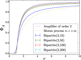
(a) Average fixation probabilities for $K_{2,10}$, $K_{2,50}$, $K_{2,100}$ and $K_{2,200}$

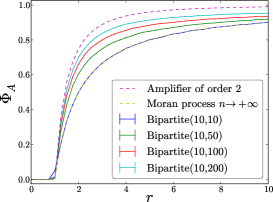
(b) Average fixation probabilities for $K_{10,10}$, $K_{10,50}$, $K_{10,100}$ and $K_{10,200}$

Figure 10: Average fixation probabilities for Moran processes on some bipartite graphs obtained from Monte Carlo methods. The same figures can be obtained from the loop-erasing method.

Proof.

We start by observing that, according to (20), we have:

$$\hat{P}_{0,j}^{\scriptscriptstyle\rightarrow}=\frac{rm_{2}}{m_{1}+rm_{2}}$$

for $1\leq j\leq m_{2}$ and

$$\hat{P}_{i,j}^{\scriptscriptstyle\rightarrow}-\hat{P}_{i,j-1}^{\scriptscriptstyle\rightarrow} =\frac{r(m_{1}-i)jm_{2}}{(m_{1}+rm_{2})(m_{1}-i)j+i(m_{2}-j)(rm_{1}+m_{2})}$$

$$\quad-\frac{r(m_{1}-i)(j-1)m_{2}}{(m_{1}+rm_{2})(m_{1}-i)(j-1)+i(m_{2}-j+1)(rm_{1}+m_{2})}$$

$$=\frac{rm_{2}}{m_{1}+rm_{2}+\dfrac{i}{m_{1}-i}\cdot\dfrac{m_{2}-j}{j}\,(rm_{1}+m_{2})}$$

$$\quad-\frac{rm_{2}}{m_{1}+rm_{2}+\dfrac{i}{m_{1}-i}\cdot\dfrac{m_{2}-j+1}{j-1}\,(rm_{1}+m_{2})}$$

$$<rm_{2}\cdot\frac{\dfrac{i}{m_{1}-i}\,\Bigl{(}\dfrac{m_{2}-j+1}{j-1}-\dfrac{m_{2}-j}{j}\Bigr{)}\,(rm_{1}+m_{2})}{(m_{1}+rm_{2})^{2}}$$

$$=rm_{2}\cdot\frac{\dfrac{i}{m_{1}-i}\cdot\dfrac{m_{2}}{j(j-1)}\,(rm_{1}+m_{2})}{(m_{1}+rm_{2})^{2}}$$

$$<rm_{2}\cdot\frac{\dfrac{i}{m_{1}-i}\,m_{2}\,(rm_{1}+m_{2})}{(m_{1}+rm_{2})^{2}}$$

for $2\leq j\leq m_{2}$ and for $1\leq i\leq m_{1}-1$. Assuming $m_{1}\geq 2i$, we have $\frac{i}{m_{1}-i}\leq 1$ and hence

$$\hat{P}_{i,j}^{\scriptscriptstyle\rightarrow}-\hat{P}_{i,j-1}^{\scriptscriptstyle\rightarrow}<rm_{2}\cdot\frac{\dfrac{i}{m_{1}-i}\,m_{2}(rm_{1}+m_{2})}{(m_{1}+rm_{2})^{2}}\leq rm_{2}\cdot\frac{m_{2}(rm_{1}+m_{2})}{(m_{1}+rm_{2})^{2}}.$$

We deduce

$$\lim_{m_{1}\to+\infty}\hat{P}_{i,j}^{\scriptscriptstyle\rightarrow}-\hat{P}_{i,j-1}^{\scriptscriptstyle\rightarrow}=0$$ (24)

for $2\leq j\leq m_{2}$ and for $i\geq 1$. Similarly, using (21), we have $\hat{P}_{0,j}^{\scriptscriptstyle\leftarrow}=0$ for $1\leq j\leq m_{2}$, $\hat{P}_{i,m_{2}}^{\scriptscriptstyle\leftarrow}=0$ for $1\leq i\leq m_{1}-1$, and

$$\hat{P}_{i,j}^{\scriptscriptstyle\leftarrow} =\frac{im_{2}(m_{2}-j)}{(m_{1}+rm_{2})(m_{1}-i)j+i(m_{2}-j)(rm_{1}+m_{2})}$$

$$=\frac{m_{2}}{(m_{1}+rm_{2})\,\dfrac{m_{1}-i}{i}\cdot\dfrac{j}{m_{2}-j}+rm_{1}+m_{2}}$$

$$<\frac{m_{2}}{rm_{1}+m_{2}}$$

for $1\leq j\leq m_{1}-1$. As before, it follows:

$$\lim_{m_{1}\to+\infty}\hat{P}_{i,j}^{\scriptscriptstyle\leftarrow}=\hat{P}_{i,m_{2}}^{\scriptscriptstyle\leftarrow}=0$$ (25)

for $1\leq j\leq m_{2}$ and for each $i\geq 1$. Next, using (22), we have $\hat{P}_{0,j}^{\scriptscriptstyle\uparrow}=0$ for $1\leq j\leq m_{2}$, $\hat{P}_{i,m_{2}}^{\scriptscriptstyle\uparrow}=0$ for $1\leq i\leq m_{1}-1$, and

$$\hat{P}_{i,j}^{\scriptscriptstyle\uparrow} =\frac{rim_{1}(m_{2}-j)}{(m_{1}+rm_{2})(m_{1}-i)j+i(m_{2}-j)(rm_{1}+m_{2})}$$

$$=\frac{ri}{(m_{1}+rm_{2})\,\dfrac{m_{1}-i}{m_{1}}\cdot\dfrac{j}{m_{2}-j}+\dfrac{i}{m_{1}}(rm_{1}+m_{2})}$$

$$<\frac{ri}{(m_{1}+rm_{2})\,\dfrac{m_{1}-i}{m_{1}}\cdot\dfrac{j}{m_{2}-j}}$$

for $1\leq j\leq m_{1}-1$. Since $\frac{1}{2}\leq\frac{m_{1}-i}{m_{1}}$ and $\frac{1}{m_{2}}<\frac{j}{m_{2}-j}$ when $m_{1}\geq 2i$ and $j\leq m_{2}-1$, we have

$$\hat{P}_{i,j}^{\scriptscriptstyle\uparrow}<\frac{2m_{2}ri}{(m_{1}+rm_{2})}$$

and therefore

$$\lim_{m_{1}\to+\infty}\hat{P}_{i,j}^{\scriptscriptstyle\uparrow}=0$$ (26)

for $1\leq j\leq m_{2}$ and for $i\geq 1$. Finally, we have:

$$\lim_{m_{1}\to+\infty}\hat{P}_{i,j}^{\scriptscriptstyle\downarrow}-\hat{P}_{i,j-1}^{\scriptscriptstyle\downarrow}=\lim_{m_{1}\to+\infty}\hat{P}_{i,j}^{\scriptscriptstyle\rightarrow}-\hat{P}_{i,j-1}^{\scriptscriptstyle\rightarrow}+\hat{P}_{i,j}^{\scriptscriptstyle\leftarrow}-\hat{P}_{i,j-1}^{\scriptscriptstyle\leftarrow}+\hat{P}_{i,j}^{\scriptscriptstyle\uparrow}-\hat{P}_{i,j-1}^{\scriptscriptstyle\uparrow}=0$$

from (24), (25) and (26). Arguing inductively on the integer $i\geq 1$, this implies that the Moran process on the bipartite graph $K_{m_{1},m_{2}}$ reduces asymptotically to the Moran process on the star $K_{m_{1},1}$ when $m_{1}\to+\infty$, and hence

$$\lim_{m_{1}\to+\infty}\Phi_{A}(K_{m_{1},m_{2}},r)-\Phi_{A}(r,K_{m_{1},1},r)=0,$$

that proves the theorem. ∎

5 Numerical experiments in complex networks

Proposition 4.1 says that the expected number of steps until absorption in the loop-erased Markov chain is smaller or equal than that in the standard one. At first glance, this seems to imply that Monte Carlo method on the EMC (EMC method from now on) will stop before Monte Carlo on the standard chain, (Standard Monte Carlo or SMC method from now on), but there is a subtle difference between what the method does theoretically and what the computer actually does.

First of all, we need to construct a weighted directed graph $\mathcal{G}$ having $2^{n}$ states. It is almost always unfeasible when $n$ is relatively large, but it is easier for highly symmetric graphs. So simulations reproduce how individuals randomly spawn and die. In the SMC method, at each step, the chance of selecting a mutant individual for reproduction is proportional to the fitness $r\geq 1$. This uniformity allows us to update the new transition probabilities in constant time. However, in the EMC method the probability of choosing each individual for reproduction depends not only on its fitness but also on the fitness of its neighbours. More precisely, the probability that a particular mutant individual $v$ leaves offspring at a particular time is proportional to the number of resident neighbours of $v$ at that time. Similarly, if $v$ is a resident individual, the probability of choosing it for reproduction is proportional to the number of mutant neighbours. Thus, if $w$ is the neighbour of $v$ chosen to die, the EMC method needs to update the transition probabilities of each neighbour of $w$. On some graphs, this may lead to longer computation times.

We compared the amount of time it takes to end the simulations for the two methods in a series of well-known complex network models. All simulations were done on a computer running MacOS X 10.9.3 with a quad-core i5 at $2.5$GHz and $8$Gb of RAM. Graph construction and manipulation was done in Sage/NetworkX [8, 20], but the simulation routines were written in C.

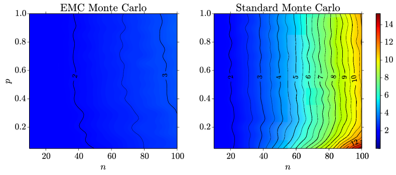
Figure 11: Average computation times (in seconds) for Moran processes on small-world networks (Watts-Strogatz $\beta$-model) using EMC and SMC methods for all $r$ going from $0$ to $10$ with step size of $0.25$.

Small-world networks

Small-world networks were introduced in [24] as a family of random graphs with some properties of real networks. The construction is as follows: consider a circular graph of order $n$ and connect the $k$ nearest neighbours. Now, each edge $uv$ in the previous graph can be replaced with another edge $uw$ with probability $p$. The resulting graph may be disconnected.

We did the following experiment to test the speed of the two methods: Fixed $k=4$, for any $n\in\{10,20,\ldots,100\}$ and $p\in\{0,0.05,\ldots,1\}$,

• we construct $10$ random graphs with parameters $n$ and $p$;

• for each of these graphs, we compute the average fixation probability using both methods $3$ times with $1000$ trials for every fitness $r$ varying from $0$ to $10$ with step size of $0.25$.

Averaging the $30$ running times of each method we get an average computation time for both algorithms on the family of small-world networks with the prescribed parameters. The results are shown in Figure 11. As can be seen, the EMC method performs better than the SMC method on this family of networks.

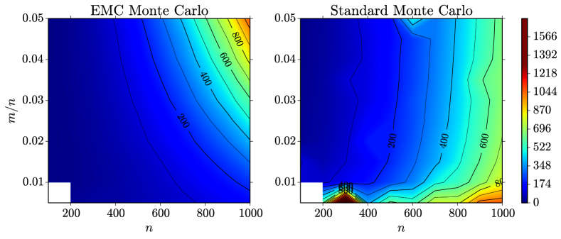
Figure 12: Average computation times (in seconds) for Moran processes on scale-free networks (Barabási-Albert preferential attachment model) using EMC and SMC methods for $r$ going from $0$ to $10$ with step size of $0.25$.

Scale-free networks

The previous family of graphs lacked a fairly common property of real networks, namely a power-law degree distribution. In [2] the preferential attachment model was developed to solve the shortcomings of previous models. Start with $m$ vertices connected in no way. Then one single vertex is added and connected to the initial vertices to obtain a star. At successive steps, another single vertex is added and connected to $m$ of the previous vertices with probability ‘proportional’ to the degree. After $n-m$ steps, the graph has $n$ vertices and $(n-m)m$ edges. In the real world, one expect to have small $m$ compared to $n$ as the global population is large and people known just a very small portion of the population.

We ran a similar experiment as for small-world networks, using both methods $3$ times for $10$ random graphs with $1000$ trials for every fitness $r$ varying from $0$ to $10$ in $40$ evenly disposed steps, but new relevant parameters are now the order of the graph $n\in\{100,200,\ldots,1000\}$ and the ratio $m/n\in\{0.005,0.01,\ldots,0.05\}$. Thus, a point $(n,m/n)$ in the plot corresponds to the average computation time on the random family with parameters $n$ and $m=\lfloor n\cdot m/n\rfloor$. The size of the population $n$ has been multiplied by $10$ with respect to the size of the small-world networks in the previous sample because we need to consider a population with $n\leq 100$ individuals if $m/n=0.01$ and $n\geq 200$ individuals if $m/n=0.005$. The result of the simulation can be seen in Figure 12. The SMC method performance is specially bad on graphs obtained by Barabási-Albert preferential attachment with $m=1$, whereas EMC method performs badly on the models with ‘large’ $m$ where high degree vertices appear. Star graphs can be interpreted as graphs obtained by Barabási-Albert preferential attachment in a single step. According to this interpretation, SMC method should improve the average computation times obtained by the EMC method. In Table 1, we compare these times on some star and complete bipartite graphs with the same number of trials and values of the fitness $r$.

Graph	EMC time	SMC time	SMC/EMC
$K_{1,10}$	1470.98	1360.97	0.99
$K_{1,50}$	1423.79	1330.04	1.26
$K_{1,100}$	1181.48	1190.43	1.05
$K_{1,200}$	1471.91	1369.67	0.93
$K_{2,10}$	1470.81	1360.88	1.09
$K_{2,50}$	1412.52	1316.17	1.29
$K_{2,100}$	1495.10	1398.49	1.04
$K_{2,200}$	1753.86	1694.88	0.92
$K_{10,10}$	1470.91	1360.90	0.99
$K_{10,50}$	1474.72	1364.53	0.96
$K_{10,100}$	1429.68	1323.68	0.80
$K_{10,200}$	1217.40	1154.32	0.71

Table 1: Average computation times (in seconds) for Moran processes on the star graphs of orders $11$, $51$, $101$ and $201$, and on the complete bipartite graphs $K_{2,10}$, $K_{2,50}$, $K_{2,100}$, $K_{2,200}$, $K_{10,10}$, $K_{10,50}$, $K_{10,100}$ and $K_{10,200}$. All simulations with $1000$ trials and $r$ going from $0$ to $10$ with step size of $0.25$. The last column shows how many times faster EMC is than the SMC method.

Hierarchical networks

In [15], a deterministic network was introduced as a heuristic model of metabolic networks (it can be seen in Figure 13). The graph has a power law distribution of the degree (scale-free topology) and mean clustering coefficient non-decreasing with size.

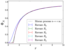
Figure 13: (a) Third step in the construction of a hierarchical network by [15], and (b) fixation probability for different construction steps compared with the Moran process as $n\to+\infty$. Here $100\,000$ trials was carried out to obtain a less noisy approximation of the fixation probability.

The network is constructed inductively. In the first step, we define the network $R_{0}$ as the complete graph of order four $K_{4}$. Fix one vertex as the central vertex. The rest of the vertices are external vertices. Now, take three copies of $R_{0}$ and join their external vertices with the central one of the original $R_{0}$ and their central vertices together making a big triangle. The central vertex of the resulting graph $R_{1}$ is the central vertex of the original $R_{0}$. The external vertices of $R_{1}$ are the vertices of the other copies of $R_{0}$. You can repeat the process as many times as needed, obtaining graphs $R_{n}$ of order $4^{n+1}$.

We computed the average fixation probability and the average computation time on this family for the same values of fitness and trials as before. The results can be seen in Figure 13 and Table 2. As one can see, the EMC method outperforms the SMC method by an increasing factor on the order $n$ of the network.

Table 2: Average computation times (in seconds) for Moran processes on the hierarchical model by [15] using EMC and SMC methods, both with $1000$ trials and $r$ going from $0$ to $10$ with step size of $0.25$. The last column shows how many times faster EMC is than the SMC method.

Step	Graph order	EMC time	SMC time	SMC/EMC
$0$	$\phantom{121}4$	$\phantom{70}0.76$	$\phantom{692}0.82$	$1.07$
$1$	$\phantom{12}16$	$\phantom{70}0.88$	$\phantom{692}0.94$	$1.06$
$2$	$\phantom{12}64$	$\phantom{70}1.92$	$\phantom{692}5.15$	$2.68$
$3$	$\phantom{1}256$	$\phantom{7}24.94$	$\phantom{6}141.24$	$5.66$
$4$	$1024$	$707.61$	$6923.04$	$9.78$

6 Conclusion

In this paper, we review some fundamental ideas and results on evolutionary dynamics as introduced in [11] generalising the classic process described in [12]. But we also give insights on one of the major problems in this theory, to estimate the average fixation probability of a mutant with relative fitness $r$ on a given graph. Exact solutions have only been computed for a few families of graphs [3] as, generally, one should solve a linear equation systems of $2^{N}$ equations, where $N$ is the order of the graph. Even asymptotic behaviour is tricky to compute.

The erasing of loops in the state space is the geometrical counterpart of a well known device in Markov chains, which is the basis behind embedded processes and which consists of forcing the processes to evolve in each iteration. It is rather obvious and well known that the expected fixation time is reduced and the fixation probability is unchanged by this procedure. In this paper, we use this idea to compute asymptotically the fixation probability for the class of complete bipartite graphs, generalising the result of [11] for the star graph. In this case, the high degree symmetry reduces the problem to a set of $2N$ equations, which is asymptotically equivalent to a simpler linear system of $N$ equations. For complete bipartite graphs, after erasing all non-trivial loops, partial symmetries arise asymptotically in the Moran process and reduce the Moran process to the particular case of a star graph. This is an important step since it shed some new light on the asymptotic behaviour of the fixation on bipartite graphs, which has recently been dealt with from other points of view in [9] and [21].

In practice, the Monte Carlo on the Embedded Markov chain (EMC method) may need to make more computations than the Monte Carlo method on the standard chain (SMC method), as it needs to keep track of different probabilities (one per vertex) that should be computed at runtime. We tested the speed of the new method in some celebrated families of graphs: the small world networks [24], preferential attachment networks [2] and hierarchical networks [15]. These tests show the EMC method defeats the SMC method on large families of graphs, but not in all examples, as transition probabilities on the loop-erased chain depends heavily on the actual state. At first, the appearance of high degree vertices might look like culprit for this problem, but this is not the case: the hierarchical network of [15] has extremely large degree on some vertices. Although it is still unknown what makes EMC method become slower, we believe this method could be applied successfully to real networks.

Globally, we think the present paper represents substantial progress towards understanding the complexity behind evolutionary dynamics on graphs.

E-mail addresses:

Fernando Alcalde Cuesta: fernando.alcaldecuesta@gmail.com

Pablo González Sequeiros: pablo.gonzalez.sequeiros@usc.es

Álvaro Lozano Rojo: alvarolozano@unizar.es

References

- [1] A. Banerjee. Structural distance and evolutionary relationship of networks. Biosystems, 107(3):186 – 196, 2012.
- [2] A.-L. Barabási and R. Albert. Emergence of scaling in random networks. Science, 286:509–512, 1999.
- [3] M. Broom and J. Rychtář. An analysis of the fixation probability of a mutant on special classes of non-directed graphs. Proc. R. Soc. Lond. Ser. A Math. Phys. Eng. Sci., 464(2098):2609–2627, 2008.
- [4] M. Broom, J. Rychtář, and B. T. Stadler. Evolutionary dynamics on small-order graphs. J. Intesdiscip. Math., 12:129–140, 2009.
- [5] M. Broom, J. Rychtář, and B. T. Stadler. Evolutionary dynamics on graphs—the effect of graph structure and initial placement on mutant spread. J. Stat. Theory Pract., 5(3):369–381, 2011.
- [6] J. Díaz, L. A. Goldberg, G. B. Mertzios, D. Richerby, M. Serna, and P. G. Spirakis. Approximating fixation probabilities in the generalized moran process. In Proceedings of the Twenty-Third Annual ACM-SIAM Symposium on Discrete Algorithms, SODA ’12, pages 954–960. SIAM, 2012.
- [7] C. C. Hadjichrysanthou. Evolutionary models in structured populations. PhD thesis, City University London, 2012.
- [8] A. A. Hagberg, D. A. Schult, and P. J. Swart. Exploring network structure, dynamics, and function using NetworkX. In Proceedings of the 7th Python in Science Conference (SciPy2008), pages 11–15, Pasadena, CA USA, Aug. 2008.
- [9] B. Houchmandzadeh and M. Vallade. Exact results for fixation probability of bithermal evolutionary graphs. Biosystems, 112(1):49 – 54, 2013.
- [10] S. Karlin and H. M. Taylor. A First Course in Stochastic Processes. Academic Press Inc., New York, N.Y., second edition, 1975.
- [11] E. Lieberman, C. Hauert, and M. A. Nowak. Evolutionary dynamics on graphs. Nature, 433(7023):312–316, Jan. 2005.
- [12] P. A. P. Moran. Random processes in genetics. Proc. Cambridge Philos. Soc., 54:60–71, 1958.
- [13] M. A. Nowak. Evolutionary Dynamics: Exploring the Equations of Life. Belknap Press of Harvard University Press, Sept. 2006.
- [14] M. A. Nowak, A. Sasaki, C. Taylor, and D. Fudenberg. Emergence of cooperation and evolutionary stability in finite populations. Nature, 428(6983):646–650, 2004.
- [15] E. Ravasz, A. L. Somera, D. A. Mongru, Z. N. Oltvai, and A.-L. Barabási. Hierarchical organization of modularity in metabolic networks. Science (New York, N.Y.), 297(5586):1551–1555, Aug. 2002.
- [16] J. Rychtář and B. Stadler. Evolutionary dynamics on small-world networks. International Journal of Computational and Mathematical Sciences [electronic only], 2(1):1–4, electronic only, 2008.
- [17] P. Shakarian and P. Roos. Fast and deterministic computation of fixation probability in evolutionary graphs. In In: CIB ’11: The Sixth IASTED Conference on Computational Intelligence and Bioinformatics (accepted). IASTED, 2011.
- [18] P. Shakarian, P. Roos, and A. Johnson. A review of evolutionary graph theory with applications to game theory. Biosystems, 107(2):66 – 80, 2012.
- [19] P. Shakarian, P. Roos, and G. Moores. A novel analytical method for evolutionary graph theory problems. Biosystems, 111(2):136 – 144, 2013.
- [20] W. A. Stein et al. Sage Mathematics Software (Version 5.8). The Sage Development Team, 2013. http://www.sagemath.org.
- [21] S. Tan and J. Lu. Characterizing the effect of population heterogeneity on evolutionary dynamics on complex networks. Sci. Rep., 4, may 2014.
- [22] C. Taylor, D. Fudenberg, A. Sasaki, and M. Nowak. Evolutionary game dynamics in finite populations. Bulletin of Mathematical Biology, 66(6):1621–1644, 2004.
- [23] H. M. Taylor and S. Karlin. An introduction to stochastic modeling. Academic Press Inc., San Diego, CA, third edition, 1998.
- [24] D. J. Watts and S. H. Strogatz. Collective dynamics of ‘small-world’ networks. Nature, 393(6684):440–442, June 1998.