Application of Mutual Information Methods in Time–Distance Helioseismology

Abstract

We apply a new technique, the mutual information (MI) from information theory, to time–distance helioseismology, and demonstrate that it can successfully reproduce several classic results based on the widely used cross–covariance method. MI quantifies the deviation of two random variables from complete independence, and represents a more general method for detecting dependencies in time series than the cross–covariance function, which only detects linear relationships. We provide a brief description of MI-based technique and discuss the results of the application of MI to derive the solar differential profile, a travel-time deviation map for a sunspot and a time–distance diagram from quiet Sun measurements.

1 Introduction

S-Introduction The field of local helioseismology is primarily concerned with the propagation of high-degree acoustic waves in the solar medium. For 20 years the primary method for detecting these waves has been the cross–covariance, or cross-correlation function [CCF: Duvall et al. (1993)]. While this tool has been used to great success, it does have limitations. The CCF can be thought of as a time-displaced scalar product and in some sense this works for detecting when two signals are similar to one other. However, the CCF-based method is at best a first-order approximation to quantifying the actual relationship between the signals. Here we propose an alternative tool based on information theory, specifically the mutual information (MI), which can be used to produce similar results to the CCF but allows one to characterize the amount of information transferred from one place on the Sun to the other, and thus, may represent more physical “connection” between two regions.

Since Shannon (1948) first formalized the theory of information for communication theory, it has found many uses in a wide variety of other fields ranging from biology to economics, or indeed anywhere stochastic models may be used. Shannon originally set out to find a measure [$H$] of how much uncertainty is in a random process, or how much information could be encoded in that process. He required a few basic properties of this measure such as continuity and a natural behavior with respect to probabilities, i.e. in the discrete case if all probabilities are $1/n$ then $H$ should be a monotonically increasing function of $n$ and if two outcomes should be grouped together then $H$ should be a weighted sum of the individual values of $H$ for each layer of grouping. He showed that the only measure satisfying these properties was the entropy. He then went on to find the rate of transmission of information through a channel with noise and bandwidth limitations. This idea was generalized from the rate of transmission to mutual information, which broadly describes the information or entropy which is shared by two signals, i.e. the amount of uncertainty in one signal that is due to another signal and vice versa. This gives a much more general view of correlations because it captures more dependencies.

When applied to the field of helioseismology, MI offers a new perspective on old problems, aside from providing an alternative and independent method to the CCF. For instance, by tracking the amount of information in a wavepacket as it propagates across the surface one can determine information flows, which potentially can be used in nonequilibrium thermodynamics (e.g. Sagawa and Ueda, 2012) and also to determine wavepacket lifetimes. By looking at MI between areas of the Sun, one can outline regions of information exchange, areas where the dynamics in one part of the Sun are influencing the dynamics in other, offering insight into the degree to which different parts of the solar atmosphere are connected. In this article, we explore the applicability of MI methods to local helioseismology on the Sun. We use MI to reproduce some of the results of traditional time–distance helioseismology as well as provide insights on the rate of information loss of waves in the solar atmosphere, which we then use to estimate wave lifetimes. At each step, comparison is made between the results of MI and CCF which we find to be in a good agreement. The rest of the article is organized as follows: Section sec:method introduces mutual information and its computation, and provides details of our implementation of MI to solar data. Sections sec:data – sec:discuss describe the data and discuss the results of our analysis.

2 Methodology

sec:method

2.1 Definitions and Interpretations of MI

Let us consider the time series of an acoustic source on the Sun as realizations of a random variable $X$, and the time series at a different point as realizations of a random variable $Y$. The mutual information [$I(X;Y)$] between the two random variables is defined as (e.g. Cover and Thomas, 2006)

$$I(X;Y)=\int_{Y}\int_{X}p(x,y)\log\frac{p(x,y)}{p(x)p(y)}{\mathrm{d}}x{\mathrm{d}}y,\ilabel{midef}$$ (1)

where the integral is taken over all possible outcomes [$x$ and $y$] with probability distributions $p(x)$ and $p(y)$, and joint probability $p(x,y)$. The base of the logarithm defines the units of information, and in this article we take the bases of all logarthims to be the natural one, corresponinding to natural units of information [nats]. An alternate relation describes MI in terms of the entropy of the source [$H(X)$] and the conditional entropy, [$H(X\big{|}Y)=-\int p(x,y)\log p(x\big{|}y)$] of the source when the other signal is known, or vice versa

$$I(X;Y)=H(X)-H(X\big{|}Y)=H(Y)-H(Y\big{|}X).$$ (2)

If one thinks of the conditional entropy as the amount of information left in one signal when the other signal is known, then subtracting it from the total entropy of the signal leaves the amount of information which is accounted for by the other signal. One last useful relation gives MI in terms of the entropies of the signal and the joint entropy, [$H(X,Y)=-\int p(x,y)\log p(x,y)$] of the two signals

$${I(X;Y)=H(X)+H(Y)-H(X,Y)}.\ilabel{MIjoint}$$ (3)

If we think of the entropy as the uncertainty in a random variable, then the MI captures the reduction in uncertainty of one random variable due to the presence of the other. Since the maximum uncertainty two variables can have is the sum of the uncertainties of the two variables (knowing one variable does not make the other more random), it is easy to see that $I(X;Y)\geq 0$ since $H(X,Y)\leq H(X)+H(Y)$ with equality only in the case of complete independence.

The manner in which the joint probability distribution is used instead of its covariance captures more complicated relationships between the two signals than the linear CCF. The ratio of the joint probability to the product of the marginal probabilities is a measure of deviations from complete independence. We can see that MI is the expectation of the logarithm of this ratio. If two signals are completely independent then this ratio is exactly 1 and the MI is zero. To see how the MI behaves under linear correlations one can consider two correlated Gaussian random variables with zero mean. The covariance matrix will be

$$\Sigma=\left(\begin{array}[]{cc}\langle X^{2}\rangle&\langle XY\rangle\\ \langle XY\rangle&\langle Y^{2}\rangle\\ \end{array}\right).$$ (4)

The entropy of a univariate Gaussian is $H(X)=\frac{1}{2}\log(2\pi e\langle X^{2}\rangle)$ and for the multivariate case of $n$ variables with covariance matrix $\Sigma$ is $H(X_{1},...,X_{n})=\frac{1}{2}\log\left(\left(2\pi e\right)^{n}\big{|}\Sigma\big{|}\right)$ which means by Equation (MIjoint) that the MI for our case of two variables is

$$I(X;Y) = \frac{1}{2}\log\left(2\pi e\langle X^{2}\rangle\right)+\frac{1}{2}\log\left(2\pi e\langle Y^{2}\rangle\right)$$ (5)

$$\;-\frac{1}{2}\log\left[\left(2\pi e\right)^{2}\left(\langle X^{2}\rangle\langle Y^{2}\rangle-\langle XY\rangle^{2}\right)\right]$$

$$= -\frac{1}{2}\log\left(1-\frac{\langle XY\rangle^{2}}{\langle X^{2}\rangle\langle Y^{2}\rangle}\right),$$

and thus the MI is a simple function of the linear correlation between the variables. In this notation we can write the CCF as

$$C(\tau)=\frac{\langle X_{t}Y_{t+\tau}\rangle}{\sqrt{\langle X^{2}\rangle\langle Y^{2}\rangle}},\ilabel{ccfdef}$$ (6)

where we’ve indexed the realizations of the random variable by time and taken the time average. For weakly correlated Gaussians we might then expect that

$$I(\tau)\approx C(\tau)^{2}.\ilabel{ccfsq}$$ (7)

2.2 Calculating MI

The simplest algorithms for MI use histograms to calculate the probability distributions. This approach has the advantage of speed, although it results in an answer that may depend on the binning procedure used, as in Leontitsis (2001) where the histogram method is used to derive the mutual average information. In order to accurately calculate the MI between two signals, we turn to an approach which uses a $k$-nearest neighbor algorithm for estimating the probability distribution (Kraskov, Stögbauer, and Grassberger, 2004). This algorithm, as opposed to simple nearest neighbor algorithms (Kozachenko and Leonenko, N. N., 1987; Victor, 2002), has the advantage that by choosing $k$ one can tune the amount of systematic error versus the amount of statistical error present in the answer. Kraskov, Stögbauer, and Grassberger (2004) found empirical scaling laws based on $k/N$ and recommend using a $k$ between $2-4$. The disadvantage of using MI in time–distance helioseismology is that the signals are typically shorter than the ideal statistical sample. For quiet-Sun calculations the problem can be alleviated by stringing multiple days together, but for active-Sun calculations such as detecting sunspot phase travel time deviations, the amount of data is limited by the amount of time the sunspot is visible. Nevertheless, as we demonstrate below, despite not having an optimal statistical sample MI can successfully be used to calculate travel time deviations in sunspots.

When applying the MI method, we follow a similar recipe as in the CCF–based time–distance method. First, we choose a point on the Sun as an acoustic source and measure waves propagating outward from the source by looking for time sensitive correlations in the signal of the source and the averaged signal of an annulus centered at the source. Ideally, one would compare the source with every point on the annulus centered at the source, but this would require a much faster computer than the ones that were available to us at the time of this project. In helioseismology with the CCF, the signals are compared to time displaced versions of the other. Here we use the time-displaced signals to construct a joint signal [$Z$] for which we then find the probability distributions. A point in $Z$ consists of the Cartesian product of a point from the source and a point from the annulus. We pair them up according to the time we are looking at for wave propagation, the correlations are maximum when the time is exactly the time it takes for a physical wave to travel the distance between the annulus and the source. Rather than use a histogram to get the probability density, an approach which depends on the binning procedure and may not converge, we used the algorithm of Kraskov, Stögbauer, and Grassberger (2004), which uses the probability [$P_{k}(\epsilon)$] that there are $k-1$ neighbors in the neighborhood defined by the distance [$\epsilon/2$] to the $k$th neighbor. Using this probability it is possible to construct an estimate of the probability mass [$\rho_{i}(\epsilon)$] of the $\epsilon$–neighborhood, which is assumed constant throughout the entire $\epsilon$–neighborhood [$\rho_{i}(\epsilon)\approx\epsilon^{2}p(Z_{i})$ for the joint entropy and $\rho_{i}(\epsilon)\approx\epsilon p(X_{i})$ for the marginal entropy]. Using $P_{k}(\epsilon)$, it can be shown that $\langle\log p_{i}\rangle=\psi(k)-\psi(N)$, where $\psi(x)=\frac{\mathrm{d}}{\mathrm{d}x}\log\Gamma(x)$ is the digamma function, and the problem is then reduced to finding the expectation of $\log\epsilon_{i}$, which will be expressed in terms of the number of points within 1D Euclidean neighborhoods with radius equal to the $k$th nearest neighbor distance. The maximum norm is chosen as a measure of distance, where the distance between points $(x_{1},y_{1})$ and $(x_{2},y_{2})$ is given by

$$d=\max\left\{\big{|}x_{2}-x_{1}\big{|},\big{|}y_{2}-y_{1}\big{|}\right\}.$$ (8)

The maximum norm is chosen because it has a square $\epsilon$–neighborhood, which simplifies the calculation. The length of the signal is such that a simple sorting algorithm can be used, in which the points are sorted in one direction, say $x$, and a running list of neighbors, sorted under the maximum norm, is kept. The search stops when the distance of the next point in the $x$-direction exceeds the distance in the maximum norm of the $k$th nearest neighbor. The next part of the calculation involves finding the number of neighbors [$n_{x}(x,y)$ and $n_{y}(x,y)$] within the one-dimensional Euclidean neighborhoods of $x$ and $y$ defined by the $k$th nearest neighbor distance [$d_{k}(x,y)$]. The calculated MI [$\hat{I}(X;Y)$] is then given by

$$\hat{I}(X;Y)=\psi(k)-\langle\psi(n_{x}+1)+\psi(n_{y}+1)\rangle+\psi(N),\ilabel{micalc}$$ (9)

where $N$ is the length of the time series, and the brackets denote the expectation value taken over the entire time series.

2.3 Application of MI to Helioseismology

When the signal from the point and the signal from the arc are paired up for different times $\tau$, and the MI [$\hat{I}(\tau)$] is calculated for the joint signal one needs to fit a function to extract meaningful information. Based on Equation (ccfsq) we adopt a representation of MI by (approximately) the square of the Gabor wavelet currently used for the CCF,

$$\hat{I}(\tau)\approx A\cos^{2}\left(2\pi\nu\left(\tau-\tau_{p}\right)\right)\exp\left(\frac{\tau-\tau_{g}}{2\sigma}\right)^{2}+B,\ilabel{cos2}$$ (10)

where $A$ is the amplitude of the wavelet, $\nu$ is the frequency corresponding to the five-minute oscillations, $\tau_{p}$ is the phase time, $\tau_{g}$ is the group time, $\sigma$ describes the width of the wavelet, and $B$ is a generally small but non-zero constant describing the average contribution from higher order correlations. Once fitted, the parameters can be used to calculate travel-time deviations as a response to flows, and even the information lost as the wave travels and correlations are destroyed. We suspect that this function reveals a property of the joint probability distribution in that it is well modeled by Gaussians, but the actual distribution is more complicated as the value of MI does not quite equal the square of the CCF. A more rigorous derivation would require the analytical form of the joint probability density function for each $\tau$. The probability density is easy to work with on computational problems but finding an analytical form for it is not a trivial task, and is beyond the scope of this paper.

3 Data

sec:data

In this study we use medium $\ell$ [0 – 300] spherical harmonic (SH) time series from the Michelson Doppler Imager (MDI, Scherrer et al., 1995) onboard the Solar and Heliospheric Observatory (SOHO, Scherrer et al., 1995). SH coefficients for these $\ell$, though they are derived from the full disk, contain information about localized propagating wavepackets. Time–distance analyses are based on cross–covariance measurements between different locations separated by some angular distance on the solar surface. Acoustic waves with the same horizontal phase speed propagate along approximately the same raypath in the solar interior (Duvall et al., 1993). In order to isolate acoustic waves within a particular wave packet bouncing with a particular travel distance, we perform phase-speed filtering of the SH coefficients. This procedure is well accepted and widely used in local helioseismology. To obtain filtered velocity images, we chose a specific phase velocity [$\omega/k_{h}$], took the product of it with each SH time series in the Fourier domain, and performed the inverse Fourier transform. Using filtered SH coefficients, we reconstructed velocity images containing waves which propagate to a certain range of distances from a given location. Details of such filtering are described by Kholikov and Hill (2014) and Kholikov, Serebryanskiy, and Jackiewicz (2014).

To demonstrate the sensitivity of the MI technique to acoustic travel-time perturbations and solar subsurface flows, we performed three types of measurements: a calculation of the solar differential profile, a map of sunspot travel-time deviations, and a time–distance diagram in quiet Sun.

Mean travel times can be measured using the center-to-annuli scheme. For this purpose an MDI time series on 23 October 2003 was used. Filtered and reconstructed velocity images centered on AR 10484 were generated to measure travel times within and around the active region. Velocity images are tracked relative to the noon time according to the solar differential-rotation rate. In order to measure travel-time differences in the East-West direction, 15 daily velocities were reconstructed without tracking. To avoid projection effects due to the tilt of the ecliptic with respect to the solar equatorial plane [or $B_{0}$–angle], several days around the time period when $B_{0}$ was close to zero were used. To produce multi-bounce time–distance measurements, three consecutive days of quiet regions are used in 1996, also around the $B_{0}=0$ time period. These three days of data were tracked relative to the middle of the time period. The details on the data used for these three tests are listed in Table 1.

Table 1.: Dates and phase-speed filter parameters of MDI time series used

Date	Central $\ell$	Phase speed [$\mu$Hz $\ell^{-1}$]	$\Delta$ range [deg.]	Used purpose
23 Oct. 2003	140	20.5	7-10	sunspot
11 – 13 Jun. 1996	140, 210	20.5, 9.5	3-40	TD
05 – 08 Dec. 1997	140	20.5	7-10	diff. rotation
05 – 08 Dec. 1998	140	20.5	7-10	diff. rotation
05 – 07 Dec. 1999	140	20.5	7-10	diff. rotation
07 – 10 Dec. 2003	140	20.5	7-10	diff. rotation

4 Results

sec:results

In order to show the reliability of the MI method, we reproduce some of the known results from time–distance helioseismology, which were based on CCF.

4.1 Differential Rotation Profile

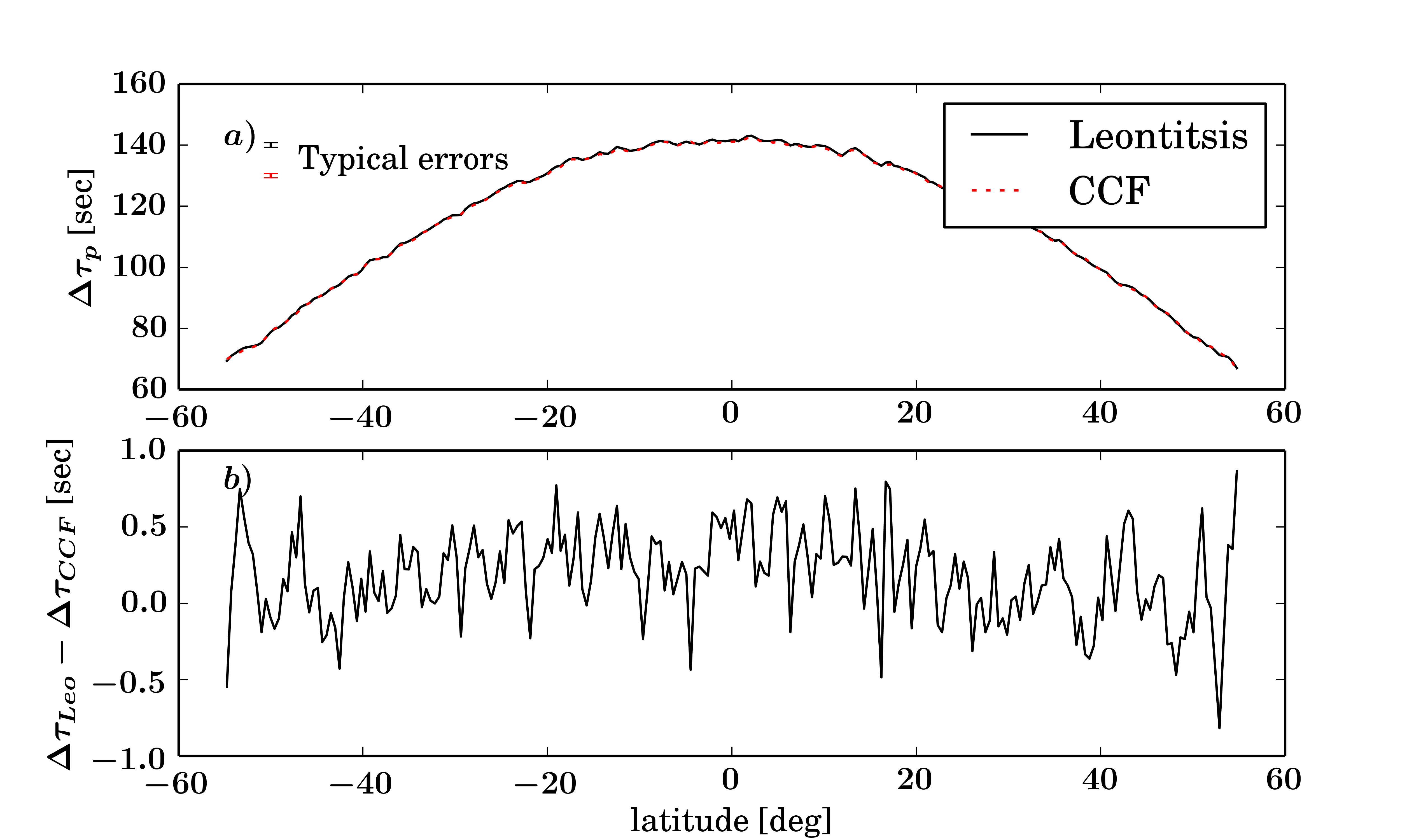
diffrot

Figure 1.: Latitudinal profile of solar rotation derived via MI and CCF methods. (a) The deviation in phase travel time [$\Delta\tau_{p}$] between east-going and west-going waves over a range of latitudes, using the mutual average information algorithm of Leontitsis and using the traditional CCF approach. (b) Difference between the phase travel-time deviations as calculated using the approach of Leontitsis, $\Delta\tau_{Leo}$, and using the CCF method, $\Delta\tau_{CCF}$.

Using the histogram method of Leontitsis (2001), we were able to quickly construct a differential rotation profile. In this case, rather than use an annulus, we used the section of the annulus which was longitudinally displaced in the direction of solar rotation. As the value given in this algorithm depends on the binning procedure, we did not make use of the amplitude but merely fit a cosine–squared wavelet and looked for deviations in the phase travel-time difference between east-going and west-going waves. Each step in the analysis is as follows

1. For each point, get a time series $X_{t}$ from the data cube.

2. Calculate the average time series for an arc displaced in the direction of solar rotation, $Y_{t}$.

3. For each $\tau$ calculate the probability densities using histograms for $X_{t}$, $Y_{t+\tau}$ and the joint signals $(X_{t},Y_{t+\tau})$ and $(X_{t+\tau},Y_{t})$ for east-traveling and west-traveling waves respectively.

4. Using these probability densities calculate $\hat{I}(\tau)$ from Equation (midef) and calculate $C(\tau)$ from Equation (ccfdef).

5. Average $\hat{I}(\tau)$ and $C(\tau)$ over longitude to get a series for each latitude.

6. Extract the phase times, $\tau_{p}$ from the fit of Equation (cos2). And subtract the east-traveling phase time and west-traveling phase time to see the effect of solar rotation.

In Figure 1, we show the difference in the phase travel-time for a range of latitudes. The data sets are nearly on top of each other so we do not show the error bars, but give a typical error bar in the upper-left corner, which represent errors of about 0.75 seconds for MI and 0.68 seconds for the CCF. There is a slight, systematic difference between the two sets which tends to make Leontitsis’s method give a very slightly larger value than the CCF, a difference which grows to about $0.25$ seconds at low latitudes and decreases for larger latitudes.

4.2 Sunspot Travel-Time Deviations

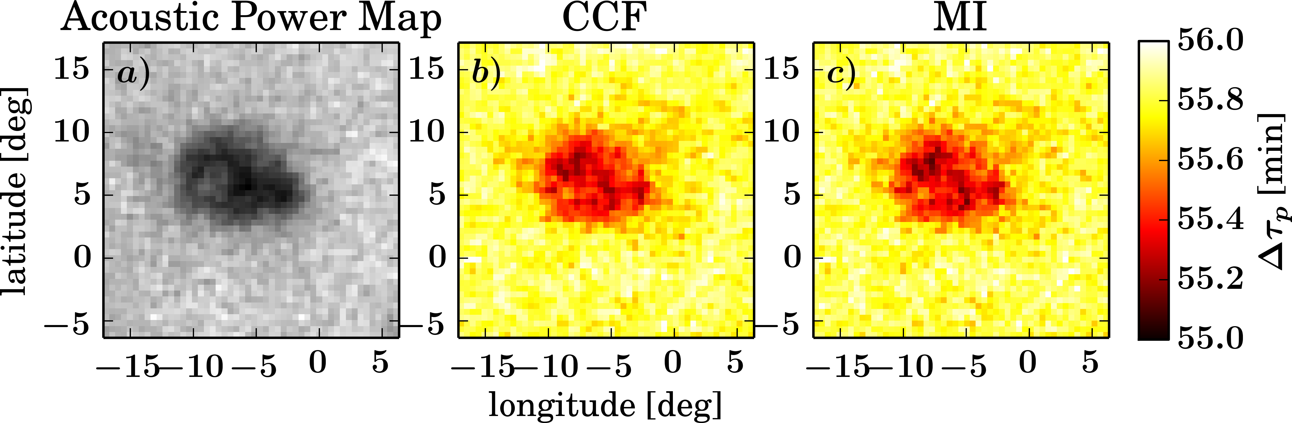
Figure 2.: (a) A map of acoustic power showing the structure of AR 10484 as a comparison to the travel-time maps. (b) Travel-time deviation map calculated using the CCF method. (c) Travel-time deviation map calculated using the $k$-nearest neighbor MI method.spotfig

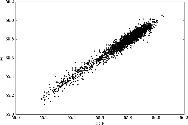
Figure 3.: Scatter plot of travel-time deviations (in units of minutes) due to AR 10484 for MI and CCF.scatter

Using the $k$-nearest neighbor approach we generated a phase travel-time deviation map of an active region. Figure spotfig shows a phase travel-time map for AR 10484, on 23 October 2003, as well as an acoustic power map for the day as a comparison. The active region is seen as a decrease in phase travel-time for outward–traveling waves, by about 20 – 40 seconds – a result consistent with previous findings (Kholikov, 2004). The annuli were chosen with radii of $7.54^{\circ}$, $8.47^{\circ}$, and $9.41^{\circ}$, so that there was minimal overlap between the active region and the annuli. The analysis went as follows

1. Generate data cube for tracked sunspot.

2. For each point, get time series $X_{t}$ and averaged time series $Y_{t}$ for the annulus at the three distances.

3. Calculate $C(\tau)$ and fit Gabor wavelet and extract phase time.

4. (MI) Generate cartesian product for a given $\tau$, $Z=(X_{t},Y_{t+\tau})$.

5. (MI) Sort data by first dimension. For each point [$(x_{i},y_{i})$], check neighbors and keep list of $k$ neighbors sorted under the maximum norm. When the distance from the point to its next neighbor is bigger than the $k$th neighbor under the maximum norm, the $k$th nearest neighbor is found. Get distance $d_{k}(x_{i},y_{i})$.

6. (MI) For each point, count how many points fall in the 1D neighborhoods of size $d_{k}(x_{i},y_{i})$, call it $n_{x}(x_{i},y_{i})$ for the first dimension and $n_{y}(x_{i},y_{i})$ for the second dimension.

7. (MI) Calculate $\psi(n_{x}(x_{i},y_{i})+1)$ and $\psi(n_{y}(x_{i},y_{i})+1)$ for each point and average values over the entire time series.

8. (MI) Plug into Equation (micalc) to get $\hat{I}(\tau)$. Repeat for each $\tau$.

9. (MI) Fit Equation (cos2) to $\hat{I}(\tau)$ series and extract phase time

10. Average phase time for three distances.

Other parameters are affected by the presence of the active region, such as group travel time; however, none of the other parameters provide the level of definition that the phase travel-time map offers. The extent of the region is fully covered by the travel-time map, and to a lesser extent so are some of the interior and edge structures. The values given by the CCF and MI methods are in good agreement as can be seen in Figure scatter, where the points are distributed closely around the diagonal.

4.3 Time–Distance Diagram

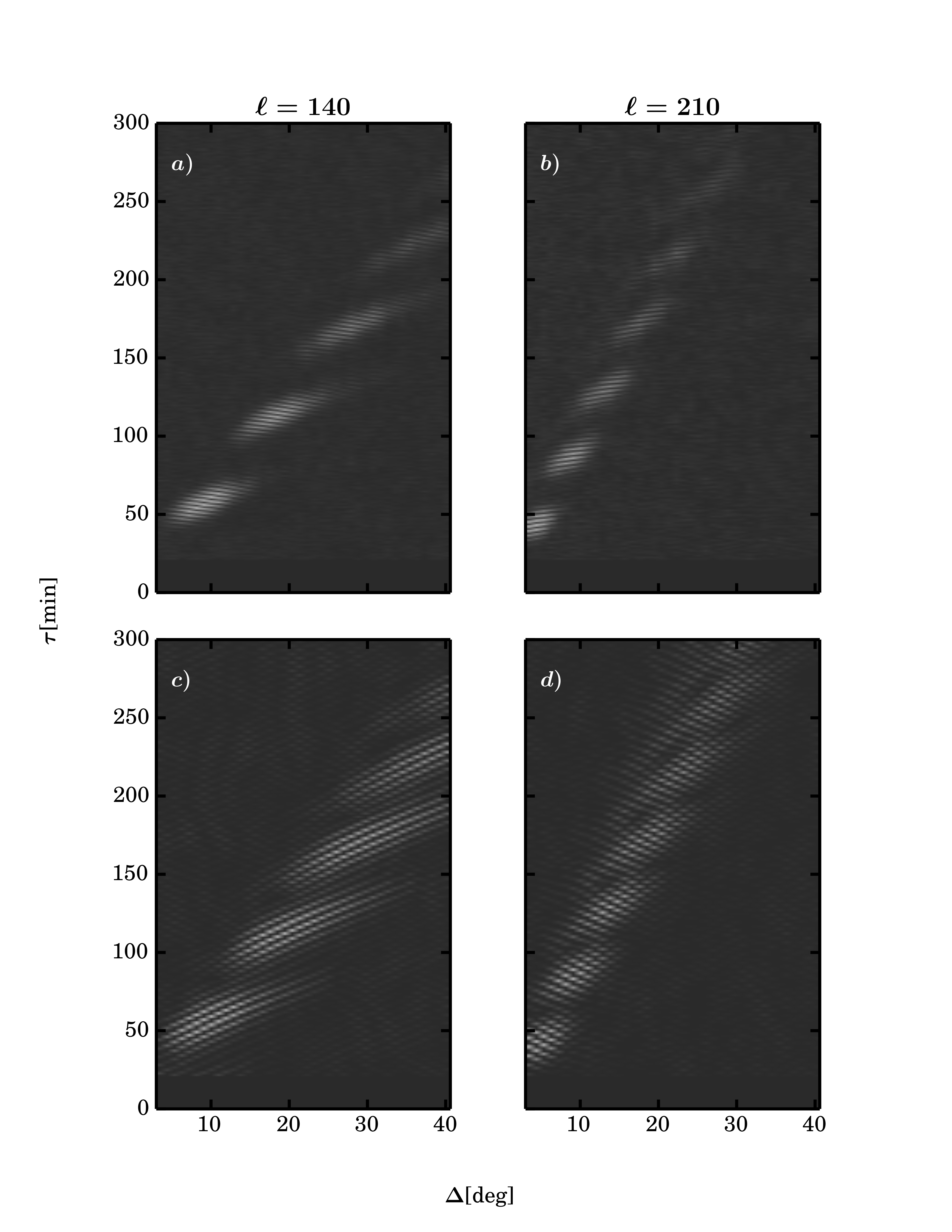
tdfig

Figure 4.: (a) MI time–distance diagram for $\ell=140$, (b) MI time–distance diagram for $\ell=210$, (c) CCF time–distance diagram for $\ell=140$, (d) CCF time–distance diagram for $\ell=210$.

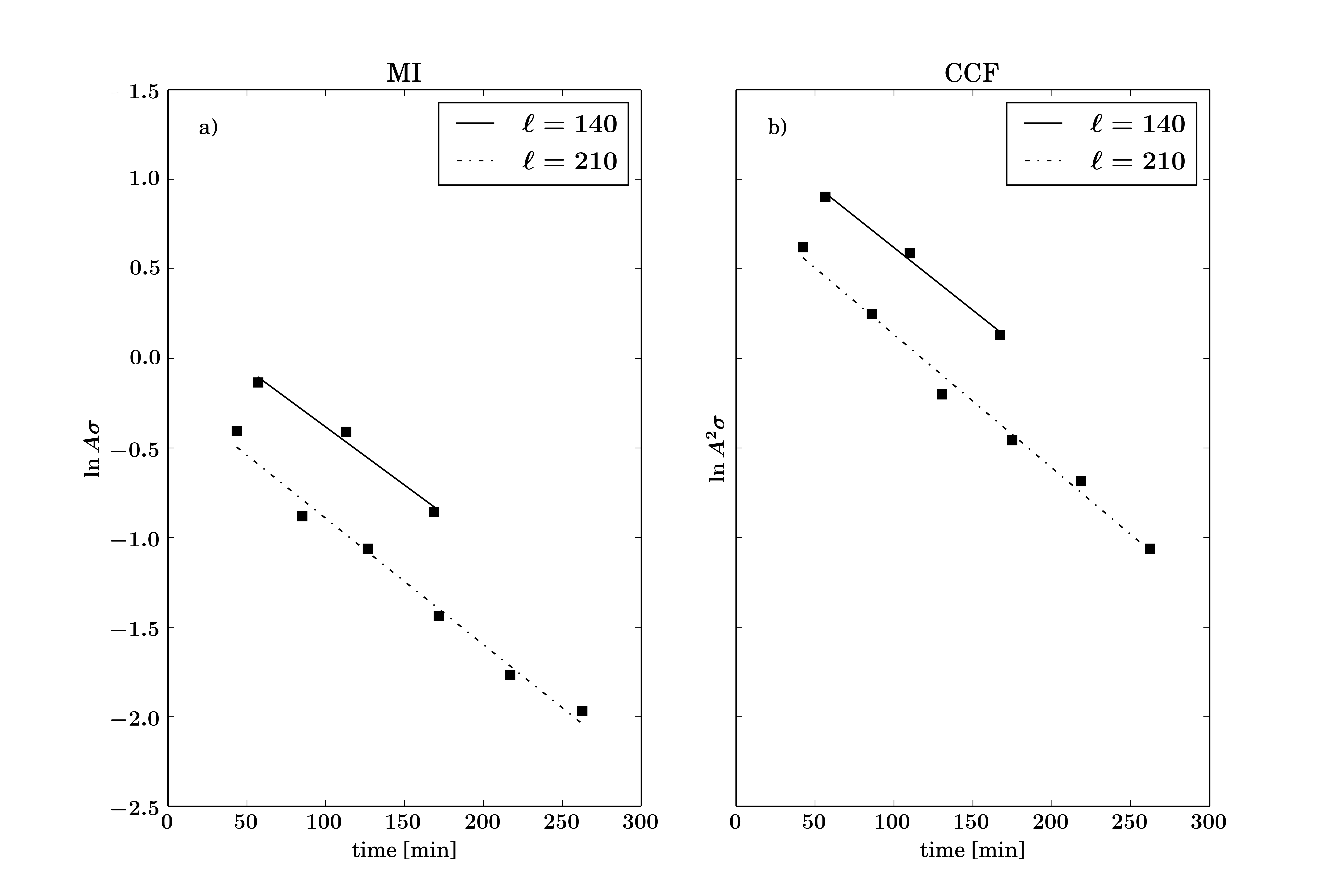
lifetime

Figure 5.: (a) Logarithm of amplitude of MI times the width vs. time where the amplitudes and widths are taken at the maximums of each skip. (b) Logarithm of amplitude squared of CCF times the width vs. time. The slopes are the negative of the inverse of the lifetime. For MI they are $T_{MI,140}=154.02$ min and $T_{MI,210}=141.82$ min. The CCF gives $T_{CCF,140}=143.03$ min $T_{CCF,210}=134.48$ min. The errors are on the order of about $0.6$ sec.

We generated a time–distance diagram, much like the CCF would produce, using the $k$-nearest neighbor algorithm. This data was constructed from three consecutive daily observations [4320 minutes]. The quiet region near the disk center was used to avoid any travel-time perturbations due to active regions. A central point was picked and the MI was computed with respect to annuli over varying distances. Then the calculations were repeated for a different central point, and again for a $10\times 10$ central square and the results were averaged, producing the diagrams in Figure 3. The analysis went as follows

1. Pick a central point on the Sun and get a time series $X_{t}$.

2. Starting at a distance of $3^{\circ}$, calculate the average time series, $Y_{t}$, for an annulus of width $0.94^{\circ}$.

3. (CCF) Calculate $C(\tau)$ for a range of $\tau$ from 20 – 300.

4. (MI) Calculate $\hat{I}(\tau)$ using the same process as the sunspot for the same range of $\tau$ as the CCF.

5. Repeat for distances increasing by an increment of $0.94^{\circ}$.

6. Repeat for different central point in the $10\times 10$ central square.

7. Average over central points.

The left side shows data which have been derived from filtered SH time series centered at $\ell=140$, while the right side is from filtered SH time series centered at $\ell=210$. The relation which takes into account dispersion and dissipation for the CCF is

$${\left(A^{2}\sigma\right)(t)=A^{2}_{0}\sigma_{0}\mathrm{e}^{-t/T}},$$ (11)

where $T$ is the lifetime of the wave. We expect then that the MI would approximately follow this relation with $A^{2}$ replaced by $A$, a constant change in $\sigma$ would not affect the lifetime. Figure 4 shows the respective quantities for MI and CCF for each skip on a logarithmic scale against the time of the maximum amplitude [the group time [$\tau_{g}$]] where the slope of the resulting line is $-T^{-1}$. To obtain the amplitudes, we fit Equation (cos2) to the MI data for the time around the maximum of the skip. This is the same as the method we used to get the CCF data, except that in that case a Gabor wavelet was used. The error in the amplitude is of the order of $10^{-6}-10^{-7}$ for MI and $10^{-5}$ for CCF and the error in the width is of the order of $10^{-3}-10^{-2}$ for MI and $10^{-2}-10^{-1}$ for the CCF. Both methods give a similar result for the lifetime, with MI giving an only slightly longer lifetime. For MI we have the lifetimes $T_{MI,140}=154.02$ min and $T_{MI,210}=141.82$ min, and for the CCF we have $T_{CCF,140}=143.03$ min and $T_{CCF,210}=134.48$ with errors in the range of $0.6$ sec. Both show an increase in the lifetime of the longer wavelength wave $\ell=140$ wave as expected; however, the MI lifetimes are noticeably longer than the CCF lifetimes.

5 Discussion

sec:discuss

In Sections 5.1 and 5.2 we showed that MI, and MI-like, measures can be used to reproduce some of the well-known results of helioseismology based on the CCF, and in Section 5.3 we showed that MI can produce a time–distance diagram which can be used to calculate the rate of information loss and wave lifetimes. There has been work done using the CCF to calculate wave lifetimes (e.g. Chou et al., 2001; Burtseva et al., 2007), but in order to ensure consistency we calculated our own lifetimes for the CCF. We found that MI gives a slightly longer lifetime, suggesting that the lifetime of linear correlations which the CCF quantifies is slightly shorter than the lifetime when taking into account nonlinear correlations. Both MI and CCF values fall in line with other results, such as that of Chen, Chou, and TON Team (1996), which gives a lifetime of an $\ell=205$ wave to be about 1.5 – 3 hours, based on the absorption of the waves in sunspots.

The CCF is easier to work with than MI, but MI brings a more physical and complete picture. We see that for phase–time calculations the two methods are in excellent agreement. For the phase travel time deviations due to AR 10484, the values are in very good agreement (see, Figure scatter). In the sunspot, the phase time deviation value is about $-$40 seconds on the inside and $-$20 seconds on the edge of the spot. These phase time deviation values may be interpreted as a result of outward (Evershed) flows, from the point inside the sunspot to an annulus outside. But when the amplitudes are used, the two methods give slightly different answers, which is to be expected as the quantities are capturing different qualities of the wave. The fact that the MI lifetime is longer means that nonlinear correlations persist longer than linear correlations..

There has been some work in tracking information flow and its relationship to thermodynamic properties for very simple systems (e.g. Sagawa and Ueda, 2012; Barato, Hartich, and Seifert, 2013a, b; Horowitz and Esposito, 2014). These authors attempt to derive the relationship between information theoretic entropy flow and thermodynamic information flow. In equilibrium situations the two quantities are one and the same (Jaynes, 1957), but for nonequilibrium situations their relationship will depend on the system under consideration. As this is a young field, there has not been much work on systems where the states of the system are drawn from a continuum, as are velocity measurements, and not a discrete space; however, one can already see the beginnings of a framework in which one can talk about the energetics of information flow.

In this work, we generate a phase–time differential-rotation profile, calculate the phase travel time deviation due to a sunspot, and calculate the rate of information loss as a wavepacket travels through the chaotic solar atmosphere, representing the lifetime of the wavepacket. For the differential-rotation profile we tested the algorithm of Leontitsis (2001). The $k$-nearest neighbor algorithm was tested on the sunspot data, and then again to generate a time–distance diagram like the CCF method would produce, from which we derive the wavepacket lifetimes. It must be kept in mind that the MI values given here are the observed MI values, not the physical MI values for the Sun. The data that we used have a cadence of one minute and a resolution of 0.47 degrees per pixel, so that the velocity field is coarse-grained even before we introduce annuli. This is the same as applying a discretization and averaging filter to the physical data. To get more realistic values of MI would require a cadence and resolution smaller than the dynamic ranges of the Sun. This needs to be explored using data from instruments such as the Solar Dynamic Observatory/Helioseismic and Magnetic Imager (SDO/HMI) and the upcoming Daniel K. Inouye Solar Telescope (DKIST, formerly the Advanced Technology Solar Telescope, ATST).

This work represents a proof-of-concept approach to MI. The aim was to demostrate that the new method (MI) can successfully reproduce the known results of helioseismology found with the CCF, as well as provide a different physical perspective. There are many avenues for future research. The first, most obvious, project would be a systematic study of information loss for a wide range of wavelengths and distance scales, paying attention to all the parameters of the wavepacket, as the amplitude and group time were being affected by the sunspot. In stochastic modeling, two-point correlation functions are used as a measure of the correlation of random variables. This provides insight only to the level of linear correlation in the random variables. MI is a better measure because a value of zero is a definite sign of independence, whereas one would have to look at all of the higher moments to arrive at the same conclusion using correlation functions. MI is derived from a more general view of correlations which allows it to account for nonlinear relationships.

Though MI is relatively simple to use computationally, it is more difficult to use analytically as the joint probability density function must be found, using either a stochastic model or from basic assumptions about the system. This kind of analysis would be a good place to start future research. These are just a few of the ways information theory can be applied in solar physics.

Acknowledgements

NSO is operated by the Association of Universities for Research in Astronomy (AURA, Inc.), under a cooperative agreement with the National Science Foundation (NSF). The SOHO/MDI data used here are provided by the SOHO/MDI consortium. SOHO is a project of international cooperation between ESA and NASA. The authors thank anonymous referee for his/her suggestions that allowed the authors to improve the article.

References

- Barato, Hartich, and Seifert (2013a) Barato, A.C., Hartich, D., Seifert, U.: 2013a, Information-theoretic versus thermodynamic entropy production in autonomous sensory networks. Phys. Rev. E 87(4), 042104. DOI.
- Barato, Hartich, and Seifert (2013b) Barato, A.C., Hartich, D., Seifert, U.: 2013b, Rate of Mutual Information Between Coarse-Grained Non-Markovian Variables. Journal of Statistical Physics 153, 460. DOI.
- Burtseva et al. (2007) Burtseva, O., Kholikov, S., Serebryanskiy, A., Chou, D.-Y.: 2007, Effects of Dispersion of Wave Packets in the Determination of Lifetimes of High-Degree Solar p Modes from Time Distance Analysis: TON Data. Sol. Phys. 241, 17. DOI.
- Chen, Chou, and TON Team (1996) Chen, K.-R., Chou, D.-Y., TON Team: 1996, Determination of the Lifetime of High-l Solar p-Modes from the Interaction of p-Mode Waves with Sunspots. ApJ 465, 985. DOI.
- Chou et al. (2001) Chou, D.-Y., Serebryanskiy, A., Ye, Y.-J., Dai, D.-C., Khalikov, S.: 2001, Lifetimes of High-l Solar p-Modes from Time-Distance Analysis. ApJ 554, L229. DOI.
- Cover and Thomas (2006) Cover, T.M., Thomas, J.A.: 2006, Elements of information theory, 2nd edn. Wiley-Interscience, Hoboken, NJ, 20.
- Duvall et al. (1993) Duvall, T.L. Jr., Jefferies, S.M., Harvey, J.W., Pomerantz, M.A.: 1993, Time-distance helioseismology. Nature 362, 430. DOI.
- Horowitz and Esposito (2014) Horowitz, J.M., Esposito, M.: 2014, Thermodynamics with Continuous Information Flow. Physical Review X 4(3), 031015. DOI.
- Jaynes (1957) Jaynes, E.T.: 1957, Information theory and statistical mechanics. Physical Review 106(4), 620. DOI.
- Kholikov (2004) Kholikov, S.: 2004, Travel Time Measurements in Sunspots. In: Danesy, D. (ed.) SOHO 14 Helio- and Asteroseismology: Towards a Golden Future, ESA Special Publication 559, 513.
- Kholikov and Hill (2014) Kholikov, S., Hill, F.: 2014, Meridional-Flow Measurements from Global Oscillation Network Group Data. Sol. Phys. 289, 1077. DOI.
- Kholikov, Serebryanskiy, and Jackiewicz (2014) Kholikov, S., Serebryanskiy, A., Jackiewicz, J.: 2014, Meridional Flow in the Solar Convection Zone. I. Measurements from GONG Data. ApJ 784, 145. DOI.
- Kozachenko and Leonenko, N. N. (1987) Kozachenko, L.F., Leonenko, N. N.: 1987, Sample estimate of the entropy of a random vector. Probl. Peredachi Inf. 23, 9. http://mi.mathnet.ru/eng/ppi/v23/i2/p9.
- Kraskov, Stögbauer, and Grassberger (2004) Kraskov, A., Stögbauer, H., Grassberger, P.: 2004, Estimating mutual information. Phys. Rev. E 69(6), 066138. DOI.
- Leontitsis (2001) Leontitsis, A.: 2001, Mutual average information, http://www.mathworks.com/matlabcentral/fileexchange/880-mutual-average-information.
- Sagawa and Ueda (2012) Sagawa, T., Ueda, M.: 2012, Fluctuation Theorem with Information Exchange: Role of Correlations in Stochastic Thermodynamics. Physical Review Letters 109(18), 180602. DOI.
- Scherrer et al. (1995) Scherrer, P.H., Bogart, R.S., Bush, R.I., Hoeksema, J.T., Kosovichev, A.G., Schou, J., Rosenberg, W., Springer, L., Tarbell, T.D., Title, A., Wolfson, C.J., Zayer, I., MDI Engineering Team: 1995, The Solar Oscillations Investigation - Michelson Doppler Imager. Sol. Phys. 162, 129. DOI.
- Shannon (1948) Shannon, C.: 1948, A mathematical theory of communication. Bell System Technical Journal 27, 379.
- Victor (2002) Victor, J.D.: 2002, Binless strategies for estimation of information from neural data. Phys. Rev. E 66(5), 051903. DOI.