Analysis and optimization of vacation and polling models with retrials

Abstract

We study a vacation-type queueing model, and a single-server multi-queue polling model, with the special feature of retrials. Just before the server arrives at a station there is some deterministic glue period. Customers (both new arrivals and retrials) arriving at the station during this glue period will be served during the visit of the server. Customers arriving in any other period leave immediately and will retry after an exponentially distributed time. Our main focus is on queue length analysis, both at embedded time points (beginnings of glue periods, visit periods and switch- or vacation periods) and at arbitrary time points.
Keywords: vacation queue, polling model, retrials

1 Introduction

Queueing systems with retrials are characterized by the fact that arriving customers, who find the server busy, do not wait in an ordinary queue. Instead of that they go into an orbit, retrying to obtain service after a random amount of time. These systems have received considerable attention in the literature, see e.g. the book by Falin and Templeton [11], and the more recent book by Artalejo and Gomez-Corral [4].

Polling systems are queueing models in which a single server, alternatingly, visits a number of queues in some prescribed order. Polling systems, too, have been extensively studied in the literature. For example, various different service disciplines (rules which describe the server’s behaviour while visiting a queue) and both models with and without switchover times have been considered. We refer to Takagi [25, 26] and Vishnevskii and Semenova [28] for some literature reviews and to Boon, van der Mei and Winands [6], Levy and Sidi [16] and Takagi [23] for overviews of the applicability of polling systems.

In this paper, motivated by questions regarding the performance modelling of optical networks, we consider vacation and polling systems with retrials. Despite the enormous amount of literature on both types of models, there are hardly any papers having both the features of retrials of customers and of a single server polling a number of queues. In fact, the authors are only aware of a sequence of papers by Langaris [12, 13, 14] on this topic. In all these papers the author determines the mean number of retrial customers in the different stations. In [12] the author studies a model in which the server, upon polling a station, stays there for an exponential period of time and if a customer asks for service before this time expires, the customer is served and a new exponential stay period at the station begins. In [13] the author studies a model with two types of customers: primary customers and secondary customers. Primary customers are all customers present in the station at the instant the server polls the station. Secondary customers are customers who arrive during the sojourn time of the server in the station. The server, upon polling a station, first serves all the primary customers present and after that stays an exponential period of time to wait for and serve secondary customers. Finally, in [14] the author considers a model with Markovian routing and stations that could be either of the type of [12] or of the type of [13].

In this paper we consider a polling station with retrials and so-called glue periods. Just before the server arrives at a station there is some deterministic glue period. Customers (both new arrivals and retrials) arriving at the station during this glue period "stick" and will be served during the visit of the server. Customers arriving in any other period leave immediately and will retry after an exponentially distributed time.

Our study of queueing systems with retrials and glue periods was at first instance motivated by questions regarding the performance modelling and analysis of optical networks. Optical fibre offers some big advantages for communication w.r.t. copper cables: huge bandwidth, ultra-low losses, and an extra dimension – the wavelength of light. Performance analysis of optical networks is a challenging topic (see e.g. Maier [17] and Rogiest [22]). In a telecommunication network, packets must be routed from source to destination, passing through a series of routers and switches. In copper-based transmission links, packets from different sources are time-multiplexed. This is often modeled by a single server polling system. In optical switches, too, one has the need for a protocol to decide which packet may be transmitted. One might again use a cyclic polling strategy, cyclic meaning that there is a fixed pattern for giving service to particular ports/stations. However, unlike electronics, buffering of optical packets is not easy, as photons cannot be stopped. Whenever there is a need to buffer photons, they are made to move locally in fiber loops. These fiber loops or fiber delay lines (FDL) originate and end at the head of a switch. When a photon arrives at the switch at a time it cannot be served, it is sent into an FDL, thereby incurring a small delay to its time of arrival without getting lost or displaced. Depending on the availability, requirement, traffic, size of photon and other such factors, the length (delay produced) of these FDLs can differ. Hence we assume that these FDLs delay the photons by a random amount of time. Also, if a packet does not receive service after a cycle through an FDL, then depending on the model it can go into either the same or a longer or a shorter or randomly to any of the available FDLs. Hence we assume that two consecutive retrials are independent of each other. This FDL feature can be modelled by a retrial queue.

A sophisticated technology that one might try to add to this is varying the speed of light by changing the refractive index of the fiber loop, cf. [19]. By increasing the refractive index in a small part of the loop we can achieve ‘slow light’, which implies slowing the packets. When a port ‘knows’ that it will soon be served, it may start the process of increasing the refractive index at FDLs and at the end of fibers of incoming packets. By doing this, it slows down the packets which arrive at the station just before the visit period of the station begins. This feature is, in our model, incorporated as glue periods immediately before the visit period of the corresponding station. Packets arriving in this glue period can be served in that subsequent visit period.

The concept of glue period is, to the best of our knowledge, new in polling systems. It may also be interpreted as a reservation period. We view a reservation period as a period in which customers can make a reservation at a station for service in the subsequent visit period of that station. In our case, such a reservation period occurs immediately before the visit period, and could be viewed as the last part, $G_{i}$, of a switchover period of length $S_{i}+G_{i}$. Ordinary gated polling could be viewed as a service discipline in which it is always possible to make a reservation for the following visit period.

The main contributions of the paper are the following. (i) For the case of a single queue with vacations and glue periods, we provide a detailed queue-length analysis at particular embedded epochs and at an arbitrary epoch. We also show how to choose the length of the glue period that minimizes the mean number of customers in the system. (ii) We also provide a detailed queue-length analysis for the $N$-queue polling case – again at particular embedded epochs and at an arbitrary epoch.

The paper is organized as follows. In Section 2 we consider the case of a single queue with vacations and retrials; arrivals and retrials only "stick" during a glue period. We study this case separately because (i) it is of interest in its own right, (ii) it allows us to explain the analytic approach as well as the probabilistic meaning of the main components in considerable detail, (iii) it makes the analysis of the multi-queue case more accessible, and (iv) results for the one-queue case may serve as a first-order approximation for the behaviour of a particular queue in the $N$-queue case, switchover periods now also representing glue and visit periods at other queues. In Section 3 the $N$-queue case is analyzed. Section 4 presents some conclusions and suggestions for future research.

2 Queue length analysis for the single-queue case

2.1 Model description

In this section we consider a single queue $Q$ in isolation. Customers arrive at $Q$ according to a Poisson process with rate $\lambda$. The service times of successive customers are independent, identically distributed (i.i.d.) random variables (r.v.), with distribution $B(\cdot)$ and Laplace-Stieltjes transform (LST) $\tilde{B}(\cdot)$. A generic service time is denoted by $B$. After a visit period of the server at $Q$ it takes a vacation. Successive vacation lengths are i.i.d. r.v., with $S$ a generic vacation length, with distribution $S(\cdot)$ and LST $\tilde{S}(\cdot)$. We make all the usual independence assumptions about interarrival times, service times and vacation lengths at the queues. After the server’s vacation, a glue period of deterministic (i.e., constant) length begins. Its significance stems from the following assumption. Customers who arrive at $Q$ do not receive service immediately. When customers arrive at $Q$ during a glue period $G$, they stick, joining the queue of $Q$. When they arrive in any other period, they immediately leave and retry after a retrial interval which is independent of everything else, and which is exponentially distributed with rate $\nu$. The glue period is immediately followed by a visit period of the server at $Q$.

The service discipline at $Q$ is gated: During the visit period at $Q$, the server serves all "glued" customers in that queue, i.e., all customers waiting at the end of the glue period (but none of those in orbit, and neither any new arrivals).

We are interested in the steady-state behaviour of this vacation model with retrials. We hence make the assumption that $\rho:=\lambda\mathbb{E}B<1$; it may be verified that this is indeed the condition for this steady-state behaviour to exist.

Some more notation:
$G_{n}$ denotes the $n$th glue period of $Q$.
$V_{n}$ denotes the $n$th visit period of $Q$ (immediately following the $n$th glue period).
$S_{n}$ denotes the $n$th vacation of the server (immediately following the $n$th visit period).
$X_{n}$ denotes the number of customers in the system (hence in orbit) at the start of $G_{n}$.
$Y_{n}$ denotes the number of customers in the system at the start of $V_{n}$. Notice that here we should distinguish between those who are queueing and those who are in orbit: We write $Y_{n}=Y_{n}^{(q)}+Y_{n}^{(o)}$, where $q$ denotes queueing and $o$ denotes in orbit.
Finally,
$Z_{n}$ denotes the number of customers in the system (hence in orbit) at the start of $S_{n}$.

2.2 Queue length analysis at embedded time points

In this subsection we study the steady-state distributions of the numbers of customers at the beginning of (i) glue periods, (ii) visit periods, and (iii) vacation periods. Denote by $X$ a r.v. with as distribution the limiting distribution of $X_{n}$. $Y$ and $Z$ are similarly defined, and $Y=Y^{(q)}+Y^{(o)}$, the steady-state numbers of customers in queue and in orbit at the beginning of a visit period (which coincides with the end of a glue period). In the sequel we shall introduce several generating functions, throughout assuming that their parameter $|z|\leq 1$. For conciseness of notation, let $\beta(z):=\tilde{B}(\lambda(1-z))$ and $\sigma(z):=\tilde{S}(\lambda(1-z))$. Then it is easily seen that

$$\mathbb{E}[z^{X}]=\sigma(z)\mathbb{E}[z^{Z}],$$ (2.1)

since $X$ equals $Z$ plus the new arrivals during the vacation;

$$\mathbb{E}[z^{Z}]=\mathbb{E}[\beta(z)^{Y^{(q)}}z^{Y^{(o)}}],$$ (2.2)

since $Z$ equals $Y^{(o)}$ plus the new arrivals during the $Y^{(q)}$ services; and

$$\mathbb{E}[z_{q}^{Y^{(q)}}z_{o}^{Y^{(o)}}]={\rm e}^{-\lambda(1-z_{q})G}\mathbb{E}[\{(1-{\rm e}^{-\nu G})z_{q}+{\rm e}^{-\nu G}z_{o}\}^{X}].$$ (2.3)

The last equation follows since $Y^{(q)}$ is the sum of new arrivals during $G$ and retrials who return during $G$; each of the $X$ customers which were in orbit at the beginning of the glue period has a probability $1-{\rm e}^{-\nu G}$ of returning before the end of that glue period.

Combining Equations (2.1)-(2.3), and introducing

$$f(z):=(1-{\rm e}^{-\nu G})\beta(z)+{\rm e}^{-\nu G}z,$$ (2.4)

we obtain the following functional equation for $\mathbb{E}[z^{X}]$:

$$\mathbb{E}[z^{X}]=\sigma(z){\rm e}^{-\lambda(1-\beta(z))G}\mathbb{E}[f(z)^{X}].$$

Introducing $K(z):=\sigma(z){\rm e}^{-\lambda(1-\beta(z))G}$ and $X(z):=\mathbb{E}[z^{X}]$, we have:

$$X(z)=K(z)X(f(z)).$$ (2.5)

This is a functional equation that naturally occurs in the study of queueing models which have a branching-type structure; see, e.g., [8] and [21]. Typically, one may view customers who newly arrive into the system during a service as children of the served customer ("branching"), and customers who newly arrive into the system during a vacation or glue period as immigrants. Such a functional equation may be solved by iteration, giving rise to an infinite product – where the $j$th term in the product typically corresponds to customers who descend from an ancestor of $j$ generations before. In this particular case we have after $n$ iterations:

$$X(z)=\prod_{j=0}^{n}K(f^{(j)}(z))X(f^{(n+1)}(z)),$$ (2.6)

where $f^{(0)}(z):=z$ and $f^{(j)}(z):=f(f^{(j-1)}(z))$, $j=1,2,\dots$. Below we show that this product converges for $n\rightarrow\infty$ iff $\rho<1$, thus proving the following theorem:

Theorem 2.1

If $\rho<1$ then the generating function $X(z)=\mathbb{E}[z^{X}]$ is given by

$$X(z)=\prod_{j=0}^{\infty}K(f^{(j)}(z)).$$ (2.7)

Proof. Equation (2.5) is an equation for a branching process with immigration, where the number of immigrants has generating function $K(z)$ and the number of children in the branching process has generating function $f(z)$. Clearly, $K^{\prime}(1)=\lambda\mathbb{E}S+\lambda\rho G<\infty$ and $f^{\prime}(1)={\rm e}^{-\nu G}+\left(1-{\rm e}^{-\nu G}\right)\rho<1$, if $\rho<1$. The result of the theorem now follows directly from the theory of branching processes with immigration (see e.g., Theorem 1 on page $263$ in Athreya and Ney [5]). ∎

Having obtained an expression for $\mathbb{E}[z^{X}]$ in Theorem 2.7, expressions for $\mathbb{E}[z^{Z}]$ and $\mathbb{E}[z_{q}^{Y^{(q)}}z_{o}^{Y^{(o)}}]$ immediately follow from (2.2) and (2.3). Moments of $X$ may be obtained from Theorem 2.7, but it is also straightforward to obtain $\mathbb{E}X$ from Equations (2.1)-(2.3):

$$\mathbb{E}X = \lambda\mathbb{E}S+\mathbb{E}Z,$$ (2.8)

$$\mathbb{E}Z = \rho\mathbb{E}Y^{(q)}+\mathbb{E}Y^{(o)},$$ (2.9)

$$\mathbb{E}Y^{(q)} = \lambda G+(1-{\rm e}^{-\nu G})\mathbb{E}X,$$ (2.10)

$$\mathbb{E}Y^{(o)} = {\rm e}^{-\nu G}\mathbb{E}X,$$ (2.11)

yielding

$$\mathbb{E}X=\frac{\lambda\mathbb{E}S+\lambda\rho G}{(1-\rho)(1-{\rm e}^{-\nu G})}.$$ (2.12)

Hence

$$\mathbb{E}Y^{(q)}=\lambda G+(1-{\rm e}^{-\nu G})\frac{\lambda\mathbb{E}S+\lambda\rho G}{(1-\rho)(1-{\rm e}^{-\nu G})}=\frac{\lambda\mathbb{E}S+\lambda G}{1-\rho},$$ (2.13)

$$\mathbb{E}Y^{(o)}={\rm e}^{-\nu G}\frac{\lambda\mathbb{E}S+\lambda\rho G}{(1-\rho)(1-{\rm e}^{-\nu G})},$$ (2.14)

$$\mathbb{E}Z=\frac{\lambda\rho G+\lambda\mathbb{E}S[\rho(1-{\rm e}^{-\nu G})+{\rm e}^{-\nu G}]}{(1-\rho)(1-{\rm e}^{-\nu G})}.$$ (2.15)

Notice that the denominators of the above expressions equal $1-f^{\prime}(1)$. Also notice that it makes sense that the denominators contain both the factor $1-\rho$ and the probability $1-{\rm e}^{-\nu G}$ that a retrial returns during a glue period.

In a similar way as the first moments of $X$, $Y^{(q)}$, $Y^{(o)}$ and $Z$ have been obtained, we can also obtain their second moment. For further use we here calculate $\mathbb{E}[X(X-1)]$:

$$\mathbb{E}[X(X-1)] = \frac{K^{\prime\prime}(1)}{(1-\rho)(1-{\rm e}^{-\nu G})(1+\rho(1-{\rm e}^{-\nu G})+{\rm e}^{-\nu G})}$$

$$+ \frac{K^{\prime}(1)[2K^{\prime}(1)(\rho(1-{\rm e}^{-\nu G})+{\rm e}^{-\nu G})+(1-{\rm e}^{-\nu G})\lambda^{2}\mathbb{E}B^{2}]}{(1-\rho)^{2}(1-{\rm e}^{-\nu G})^{2}(1+\rho(1-{\rm e}^{-\nu G})+{\rm e}^{-\nu G})},$$

where $K^{\prime}(1)=\lambda\mathbb{E}S+\lambda\rho G$ and $K^{\prime\prime}(1)=\lambda^{2}\mathbb{E}S^{2}+2\rho\lambda^{2}G\mathbb{E}S+\lambda^{3}G\mathbb{E}B^{2}+(\lambda G\rho)^{2}$.

Remark 1

Special cases of the above analysis are, e.g.:
(i) Vacations of length zero. Simply take $\sigma(z)\equiv 1$ and $\mathbb{E}S=0$ in the above formulas.
(ii) $\nu=\infty$. Retrials now always return during a glue period. We then have $f(z)=\beta(z)$, which leads to minor simplifications.

Remark 2

It seems difficult to handle the case of non-constant glue periods, as it seems to lead to a process with complicated dependencies. If $G$ takes a few distinct values $G_{1},\dots,G_{N}$ with different probabilities, then one might still be able to obtain a kind of multinomial generalization of the infinite product featuring in Theorem 2.7. One would then have several functions $f_{i}(z):=(1-{\rm e}^{-\nu G_{i}})\beta(z)+{\rm e}^{-\nu G_{i}}z$, and all possible combinations of iterations $f_{i}(f_{h}(f_{k}(\dots(z))))$ arising in functions $K_{i}(z):=\sigma(z){\rm e}^{-\lambda(1-\beta(z))G_{i}}$, $i=1,2,\dots,N$. By way of approximation, one might stop the iterations after a certain number of terms, the number depending on the speed of convergence (hence on $1-\rho$ and on $1-{\rm e}^{-\nu G_{i}}$).

2.3 Queue length analysis at arbitrary time points

Having found the generating functions of the number of customers at the beginning of (i) glue periods ($\mathbb{E}[z^{X}]$), (ii) visit periods $(\mathbb{E}[z_{q}^{Y^{(q)}}z_{o}^{Y^{(o)}}])$, and (iii) vacation periods ($\mathbb{E}[z^{Z}]$), we can also obtain the generating function of the number of customers at arbitrary time points.

Theorem 2.2

If $\rho<1$, we have the following results:

• The joint generating function, $R_{va}(z_{q},z_{o})$, of the number of customers in the queue and in the orbit at an arbitrary time point in a vacation period equals the generating function $R_{va}(z_{o})$ of the number of customers in orbit at an arbitrary time point in a vacation period and is given by

  $$R_{va}(z_{q},z_{o})=\mathbb{E}[z_{o}^{Z}]\frac{1-\tilde{S}(\lambda(1-z_{o}))}{\lambda(1-z_{o})\mathbb{E}S}.$$ (2.17)

• The joint generating function, $R_{gl}(z_{q},z_{o})$, of the number of customers in the queue and in the orbit at an arbitrary time point in a glue period is given by

  $$R_{gl}(z_{q},z_{o})=\int_{t=0}^{G}{\rm e}^{-\lambda(1-z_{q})t}\mathbb{E}[\{(1-{\rm e}^{-\nu t})z_{q}+{\rm e}^{-\nu t}z_{o}\}^{X}]\,\frac{dt}{G}.$$ (2.18)

• The joint generating function, $R_{vi}(z_{q},z_{o})$, of the number of customers in the queue and in the orbit at an arbitrary time point in a visit period is given by

  $$R_{vi}(z_{q},z_{o})=\frac{z_{q}\left[\mathbb{E}[z_{q}^{Y^{(q)}}z_{o}^{Y^{(o)}}]-\mathbb{E}[\tilde{B}(\lambda(1-z_{o}))^{Y^{(q)}}z_{o}^{Y^{(o)}}]\right]}{\mathbb{E}[Y^{(q)}]\left(z_{q}-\tilde{B}(\lambda(1-z_{o}))\right)}\frac{1-\tilde{B}(\lambda(1-z_{o}))}{\lambda(1-z_{o})\mathbb{E}B}.$$ (2.19)

• The joint generating function, $R(z_{q},z_{o})$, of the number of customers in the queue and in the orbit at an arbitrary time point is given by

  $$R(z_{q},z_{o})=\rho R_{vi}(z_{q},z_{o})+(1-\rho)\tfrac{G}{G+\mathbb{E}S}R_{gl}(z_{q},z_{o})+(1-\rho)\tfrac{\mathbb{E}S}{G+\mathbb{E}S}R_{va}(z_{q},z_{o}).$$ (2.20)

Proof.

• Follows from the fact that during vacation periods there are no customers in the queue, hence the right-hand side of (2.17) is independent of $z_{q}$, and the fact that the number of customers at an arbitrary time point in the orbit is the sum of two independent terms: The number of customers at the beginning of the vacation period and the number that arrived during the past part of the vacation period. The generating function of the latter is given by

  $$\frac{1-\tilde{S}(\lambda(1-z_{o}))}{\lambda(1-z_{o})\mathbb{E}S}.$$

• Follows from the fact that if the past part of the glue period is equal to $t$, the generating function of the number of new arrivals in the queue during this period is equal to ${\rm e}^{-\lambda(1-z_{q})t}$ and each customer present in the orbit at the beginning of the glue period is, independent of the others, still in orbit with probability ${\rm e}^{-\nu t}$ and has moved to the queue with probability $1-{\rm e}^{-\nu t}$.

• During an arbitrary point in time in a visit period the number of customers in the system consists of two parts:

  • the number of customers in the system at the beginning of the service time of the customer currently in service, leading to the term (see Remark 3 below):

    $$\frac{z_{q}\left(\mathbb{E}[z_{q}^{Y^{(q)}}z_{o}^{Y^{(o)}}]-\mathbb{E}[\tilde{B}(\lambda(1-z_{o}))^{Y^{(q)}}z_{o}^{Y^{(o)}}]\right)}{\mathbb{E}[Y^{(q)}]\left(z_{q}-\tilde{B}(\lambda(1-z_{o}))\right)};$$ (2.21)

  • the number of customers that arrived during the past part of the service of the customer currently in service, leading to the term

    $$\frac{1-\tilde{B}(\lambda(1-z_{o}))}{\lambda(1-z_{o})\mathbb{E}B}.$$

• Follows from the fact that the fraction of time the server is visiting $Q$ is equal to $\rho$, and if the server is not visiting $Q$, with probability $\mathbb{E}S/(G+\mathbb{E}S)$ the server is on vacation and with probability $G/(G+\mathbb{E}S)$ the system is in a glue phase.

∎

Remark 3

A straightforward way to prove (2.21) is to condition on the number of customers, say, $j$, in queue at the end of a glue period, and to average the number of customers in queue and in orbit over the beginnings of the $j$ services. A more elegant proof of Formula (2.21) uses the observation that typically in vacation and polling systems each time a visit beginning or a service completion occurs, this coincides with a service beginning or a visit completion. This observation yields (see, e.g., Boxma, Kella and Kosinski [9])

$$\gamma{\cal V}_{b}(z_{q},z_{o})+{\cal S}_{c}(z_{q},z_{o})={\cal S}_{b}(z_{q},z_{o})+\gamma{\cal V}_{c}(z_{q},z_{o}).$$

Here, ${\cal V}_{b}(z_{q},z_{o})$ and ${\cal V}_{c}(z_{q},z_{o})$ are the joint generating functions of the number of customers in the queue and in the orbit at visit beginnings and visit completions, respectively. Similarly, ${\cal S}_{b}(z_{q},z_{o})$ and ${\cal S}_{c}(z_{q},z_{o})$ are the joint generating functions of the number of customers in the queue and in the orbit at service beginnings and service completions, respectively. Finally, $\gamma$ is the reciprocal of the mean number of customers served per visit. Clearly,

$$\gamma=\frac{1}{\mathbb{E}[Y^{(q)}]},\quad{\cal V}_{b}(z_{q},z_{o})=\mathbb{E}[z_{q}^{Y^{(q)}}z_{o}^{Y^{(o)}}],\quad{\cal V}_{c}(z_{q},z_{o})=\mathbb{E}[\tilde{B}(\lambda(1-z_{o}))^{Y^{(q)}}z_{o}^{Y^{(o)}}],$$

and

$${\cal S}_{c}(z_{q},z_{o})=\frac{{\cal S}_{b}(z_{q},z_{o})}{z_{q}}\tilde{B}(\lambda(1-z_{o})),$$

which yields that ${\cal S}_{b}(z_{q},z_{o})$ is given by (2.21).

From Theorem 2.2, we now can obtain the steady-state mean number of customers in the system at arbitrary time points in vacation periods ($\mathbb{E}[R_{va}]$), in glue periods ($\mathbb{E}[R_{gl}]$), in visit periods ($\mathbb{E}[R_{vi}]$) and in arbitrary periods ($\mathbb{E}[R]$). These are given by

$$\mathbb{E}[R_{va}] = \mathbb{E}[Z]+\lambda\tfrac{\mathbb{E}[S^{2}]}{2\mathbb{E}[S]},$$

$$\mathbb{E}[R_{gl}] = \mathbb{E}[X]+\lambda\tfrac{G}{2},$$

$$\mathbb{E}[R_{vi}] = 1+\lambda\tfrac{\mathbb{E}[B^{2}]}{2\mathbb{E}[B]}+\tfrac{\mathbb{E}[Y^{(q)}Y^{(o)}]}{\mathbb{E}[Y^{(q)}]}+\tfrac{(1+\rho)\mathbb{E}[Y^{(q)}(Y^{(q)}-1)]}{2\mathbb{E}[Y^{(q)}]},\,\,$$

$$\mathbb{E}[R] = \rho\mathbb{E}[R_{vi}]+(1-\rho)\tfrac{G}{G+\mathbb{E}S}\mathbb{E}[R_{gl}]+(1-\rho)\tfrac{\mathbb{E}S}{G+\mathbb{E}S}\mathbb{E}[R_{va}].$$ (2.22)

Remark that the quantities $\mathbb{E}[Y^{(q)}Y^{(o)}]$ and $\mathbb{E}[Y^{(q)}(Y^{(q)}-1)]$ can be obtained using (2.3):

$$\mathbb{E}[Y^{(q)}Y^{(o)}] = \lambda G{\rm e}^{-\nu G}\mathbb{E}[X]+\left(1-{\rm e}^{-\nu G}\right){\rm e}^{-\nu G}\mathbb{E}[X(X-1)],$$

$$\mathbb{E}[Y^{(q)}(Y^{(q)}-1)] = (\lambda G)^{2}+\left(1-{\rm e}^{-\nu G}\right)^{2}\mathbb{E}[X(X-1)]+2\lambda G\left(1-{\rm e}^{-\nu G}\right)\mathbb{E}[X].$$

By combining these relations with (2.22), (2.8), (2.12) and (2.2), we obtain – after tedious calculations – the following relatively simple expression for the mean number of customers $\mathbb{E}[R]$:

$$\mathbb{E}[R]=\rho+\frac{\lambda^{2}\mathbb{E}[B^{2}]}{2(1-\rho)}+\frac{\lambda\mathbb{E}[(G+S)^{2}]}{2\mathbb{E}[G+S]}+\frac{\lambda\rho\mathbb{E}[G+S]}{1-\rho}+\lambda(\rho G+\mathbb{E}[S])\frac{{\rm e}^{-\nu G}}{(1-\rho)(1-{\rm e}^{-\nu G})},$$ (2.23)

which we rewrite for later purposes as

$$\mathbb{E}[R] = \rho+\frac{\lambda^{2}\mathbb{E}[B^{2}]}{2(1-\rho)}+\lambda\frac{\mathbb{E}[S]}{G+\mathbb{E}[S]}\frac{\mathbb{E}[S^{2}]}{2\mathbb{E}[S]}+\lambda\frac{\mathbb{E}[S]}{G+\mathbb{E}[S]}G+\lambda\frac{G}{G+\mathbb{E}[S]}\frac{G}{2}$$ (2.24)

$$+ \frac{\lambda\rho(G+\mathbb{E}[S])}{1-\rho}+\lambda(\rho G+\mathbb{E}[S])\frac{{\rm e}^{-\nu G}}{(1-\rho)(1-{\rm e}^{-\nu G})}.$$

Remark 4

(i). It should be noticed that the first two terms in the right-hand side of (2.23) together represent the mean number of customers in the ordinary $M/G/1$ queue, without vacations and glue periods. The third term represents the mean number of arrivals during the residual part of a vacation plus glue period. The fourth term can be interpreted as the mean number of arrivals during a visit period of the server (since the mean length of one cycle, i.e., visit plus vacation plus glue period, is via a balance argument seen to equal $\mathbb{E}[C]=\frac{G+\mathbb{E}[S]}{1-\rho}$, while a mean visit period equals $\rho\mathbb{E}[C]$). The fifth term is the only term involving the retrial rate $\nu$. In particular, that term disappears when $\nu\rightarrow\infty$. In the latter case, our model reduces to an $M/G/1$ queue with gated vacations, with vacation lengths $G+S$. The resulting expression for the mean number of customers coincides with formula (5.23) of [24] (see also formula (3.2.6) of [27]).
(ii). A more interesting limiting operation is to simultaneously let $\nu\rightarrow\infty$ and $G\downarrow 0$, such that $\nu G$ remains constant. The resulting model is an $M/G/1$ queue with vacations and binomially gated service; see, e.g., Levy [15]. Here, each customer who is present at the end of a vacation, will be served in the next visit period with probability $p=1-{\rm e}^{-\nu G}$. In this case, the mean number of customers in the system is given by

$$\mathbb{E}[R]=\rho+\frac{\lambda^{2}\mathbb{E}[B^{2}]}{2(1-\rho)}+\frac{\lambda\mathbb{E}[S^{2}]}{2\mathbb{E}[S]}+\frac{\lambda\rho\mathbb{E}[S]}{1-\rho}+\frac{\lambda\mathbb{E}[S](1-p)}{p(1-\rho)}.$$ (2.25)

This formula coincides with the results obtained in [15] (see e.g., formula (7.1) with $N=1$ in [15] for the mean sojourn time of customers in this model). Observe that our formula, after application of Little’s formula, does not fully agree with the mean delay expression (5.50b) in [24] and with a similar formula on p. 90 of [27]. Those mean delay expressions for the binomial gated model seem to refer to the case where customers who are not served during a visit (w.p. $1-p$) are lost; hence factors like $\frac{1}{1-p\rho}$ in those mean delay expressions.
(iii). Formula (2.24) immediately shows how the mean number of customers behaves for very small and for very large values of the glue period length $G$:

$$\mathbb{E}[R]\sim\frac{\lambda\mathbb{E}[S]}{G\nu(1-\rho)},~{}~{}~{}G\downarrow 0,$$ (2.26)

and

$$\mathbb{E}[R]\sim\frac{\lambda(1+\rho)}{2(1-\rho)}G,~{}~{}~{}G\rightarrow\infty.$$ (2.27)

We observe that the equations (2.26) and (2.27) do not involve $\mathbb{E}[B^{2}]$ and $\mathbb{E}[S^{2}]$. Hence the mean number of customers in the system is almost invariant to the variance of the service times and vacation times when $G$ is either very small or very large. In Subsection 2.4 we explore the effect of $G$ on $\mathbb{E}[R]$ more deeply.

2.4 Optimizing the length of the glue period

One of the main reasons for studying mathematical models of optical networks is to improve the performance of the system. In this model the length of the glue period is an important system design parameter. The results of the previous subsections can, e.g., be used to determine the value of $G$ which minimizes the mean number of customers in the system at any arbitrary time point. The mean sojourn time of an arbitrary customer follows from Little’s formula. Therefore we can find the value of $G$ which minimizes the mean sojourn time of an arbitrary customer.

Let us first present a sample of numerical results that we obtained for $\mathbb{E}[R]$ as a function of $G$. We consider four cases: (i) the service time distribution and vacation time distribution are exponential, (ii) the service time distribution is exponential and the vacation time is constant, (iii) the service time is constant and the vacation time distribution is exponential and (iv) the service time and vacation time are constant. In Fig 1 we take $\lambda=0.9$, $\nu=0.5$, and $\mathbb{E}S=10$, we plot $G$ vs $\mathbb{E}[R]$, for $\mathbb{E}B=1$ and $1.1.$ Note that $\mathbb{E}B=1.1$ corresponds to the heavy traffic case $\rho=0.99$.

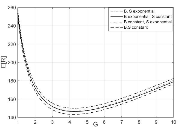
(a) $\mathbb{E}B=1$

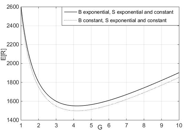
(b) $\mathbb{E}B=1.1$

Figure 1: Mean number of customers vs length of glue period

From the examples in Fig 1 we observe the following results:

• The mean number of customers at any arbitrary point seems to be convex w.r.t. glue period length, i.e., there exists a glue period $G_{min}$ where the system has minimum mean number of customers $E[R_{min}]$ and hence minimum mean sojourn time.

• For a large $G$, $\mathbb{E}[R]$ increases linearly with $G$ (as confirmed by (2.27)).

• For a very small $G$, $\mathbb{E}[R]$ behaves like $1/G$ (as confirmed by (2.26)).

• For different service time and vacation time distributions the mean number of customer is changed but the difference in $G_{min}$ is insignificantly small.

• As $\rho\rightarrow 1$ , i.e. the system is in heavy traffic regime, the value of $\mathbb{E}[R]$ becomes insensitive to the distribution of $S$.

Indeed, if $G$ is very small, the number of customers joining the queue in each glue period is very small and thereby the efficiency of the system is decreased. On the other hand, a large $G$ means the system stays in the glue period for a long time and this decreases the efficiency of the system. Hence it is logical to have a $G_{min}$ which optimizes the system.

We will now prove that $E[R]$ is indeed convex in $G$. Twice differentiating the expression for $\mathbb{E}[R]$ in Equation (2.23) w.r.t. $G$ gives

$$\frac{d^{2}}{dG^{2}}\mathbb{E}[R]=\frac{\lambda}{\mathbb{E}[G+S]}\Bigg{[}\frac{\mathbb{E}[(G+S)^{2}]}{\mathbb{E}[G+S]^{2}}-1\Bigg{]}+\frac{\lambda\nu{\rm e}^{-\nu G}}{(1-\rho)(1-{\rm e}^{-\nu G})^{2}}\Bigg{[}\nu(\rho G+\mathbb{E}[S])\frac{(1+{\rm e}^{-\nu G})}{(1-{\rm e}^{-\nu G})}-2\rho\Bigg{]}.\\$$ (2.28)

Clearly, the first term in the right-hand side of (2.28) is nonnegative. Let

$$Q(G):=\nu(\rho G+\mathbb{E}[S])\frac{(1+{\rm e}^{-\nu G})}{(1-{\rm e}^{-\nu G})}-2\rho.$$

We can see $Q(G)\longrightarrow\infty$ as $G\longrightarrow 0$ or $G\longrightarrow\infty$. Let $Q(G)$ attain its minimum at $G=g.$ Hence calculating the first derivative of $Q(G)$ and equating it to zero, at $G=g,$ gives

$$\rho g+\mathbb{E}[S]=\frac{\rho}{2\nu{\rm e}^{-\nu g}}(1-{\rm e}^{-2\nu g}).$$

Therefore

$$Q(g)=\frac{\rho}{2}[{\rm e}^{\nu g}-2+{\rm e}^{-\nu g}]\geq 0.$$

We observe that the minimum value of $Q(G)$ is always nonnegative. Since both terms of (2.28) are nonnegative, $\frac{d^{2}}{dG^{2}}\mathbb{E}[R]\geq 0.$

Hence $\mathbb{E}[R]$, the mean number of customers at an arbitrary point of time in the system, is convex in $G$. So the system can improve the quality of service by setting an optimal value of $G$ for the fixed glue period.

In Table 1 we analyze the behaviour of $G_{min}$ and $\mathbb{E}[R_{min}]$ as we increase $\mathbb{E}[S]$ for an exponential distribution $B(\cdot)$ with $\mathbb{E}B=1$, arrival rate $\lambda=0.5$ and retrial rate $\nu=0.5$.

Table 1: Optimal glue period length and corresponding minimum mean number of customers

$\mathbb{E}S$	$G_{min}$ for	$G_{min}$ for	$\mathbb{E}[R_{min}]$ for	$\mathbb{E}[R_{min}]$ for
	exponential $S(\cdot)$	constant $S(\cdot)$	exponential $S(\cdot)$	constant $S(\cdot)$
$0$	$\epsilon$,   $\epsilon\longrightarrow 0$	$\epsilon$,   $\epsilon\longrightarrow 0$	$\sim 2$	$\sim 2$
0.1	0.608	0.606	2.476	2.473
0.5	1.334	1.320	3.419	3.385
1	1.846	1.801	4.259	4.170
5	3.694	3.508	9.276	8.549
10	4.785	4.495	14.778	13.070
50	7.783	7.225	56.027	45.156
100	9.167	8.521	106.606	83.634

Table 1 suggests that, in the case under consideration,

• $G_{min}$ and $\mathbb{E}[R_{min}]$ increase when $\mathbb{E}[S]$ increases.

• $G_{min}$ and $\mathbb{E}[R_{min}]$ increase when the variance of $S$ becomes larger.

• When $\mathbb{E}S$ approaches $0$, $G_{min}$ also approaches $0$. When there is no customer in the queue, the system will then have a series of very short glue periods, and when a customer arrives or returns from orbit, it can almost instantaneously be taken into service. In this case, the system reduces to an ordinary $M/G/1$ retrial queue; indeed, Formula (2.23) reduces to $\mathbb{E}[R]=\rho+\frac{\lambda^{2}\mathbb{E}[B^{2}]}{2(1-\rho)}$ $+\frac{\lambda\rho}{\nu(1-\rho)}$ which is in agreement with Formula (1.37) of [11].

3 Queue length analysis for the N-queue case

3.1 Model description

In this section we consider a one-server polling model with multiple queues, $Q_{i},$ $i=1,\cdots,N$. Customers arrive at $Q_{i}$ according to a Poisson process with rate $\lambda_{i}$; they are called type-$i$ customers, $i=1,\cdots,N$. The service times at $Q_{i}$ are i.i.d. r.v., with $B_{i}$ denoting a generic service time, with distribution $B_{i}(\cdot)$ and LST $\tilde{B}_{i}(\cdot)$, $i=1,\cdots,N$. The server follows cyclic polling, thus after a visit of $Q_{i}$, it switches to $Q_{i+1}$. Successive switchover times from $Q_{i}$ to $Q_{i+1}$ are i.i.d. r.v., with $S_{i}$ a generic switchover time, with distribution $S_{i}(\cdot)$ and LST $\tilde{S}_{i}(\cdot)$, $i=1,\cdots,N$. We make all the usual independence assumptions about interarrival times, service times and switchover times at the queues. After a switch of the server to $Q_{i}$, there first is a deterministic (i.e., constant) glue period $G_{i}$, before the visit of the server at $Q_{i}$ begins, $i=1,\cdots,N$. As in the one-queue case, the significance of the glue period stems from the following assumption. Customers who arrive at $Q_{i}$ do not receive service immediately. When customers arrive at $Q_{i}$ during a glue period $G_{i}$, they stick, joining the queue of $Q_{i}$. When they arrive in any other period, they immediately leave and retry after a retrial interval which is independent of everything else, and which is exponentially distributed with rate $\nu_{i}$, $i=1,\cdots,N$.

The service discipline at all queues is gated: During the visit period at $Q_{i}$, the server serves all "glued" customers in that queue, i.e., all type-$i$ customers waiting at the end of the glue period – but none of those in orbit, and neither any new arrivals.

We are interested in the steady-state behaviour of this polling model with retrials. We hence assume that the stability condition $\sum_{i=1}^{N}\rho_{i}<1$ holds, where $\rho_{i}:=\lambda_{i}\mathbb{E}B_{i}$.

Some more notation:
$G_{ni}$ denotes the $n$th glue period of $Q_{i}$.
$V_{ni}$ denotes the $n$th visit period of $Q_{i}$.
$S_{ni}$ denotes the $n$th switch period out of $Q_{i}$, $i=1,\cdots,N$.
$(X_{n1}^{(i)},X_{n2}^{(i)},\cdots,X_{nN}^{(i)})$ denotes the vector of numbers of customers of type $1$ to type $N$ in the system (hence in orbit) at the start of $G_{ni}$, $i=1,\cdots,N$.
$(Y_{n1}^{(i)},Y_{n2}^{(i)},\cdots,Y_{nN}^{(i)})$ denotes the vector of numbers of customers of type $1$ to type $N$ in the system at the start of $V_{ni}$, $i=1,\cdots,N$. We distinguish between those who are queueing in $Q_{i}$ and those who are in orbit for $Q_{i}$: We write $Y_{ni}^{(i)}=Y_{ni}^{(iq)}+Y_{ni}^{(io)}$, $i=1,\cdots,N$, where $q$ denotes queueing and $o$ denotes in orbit.
Finally,
$(Z_{n1}^{(i)},Z_{n2}^{(i)},\cdots,Z_{nN}^{(i)})$ denotes the vector of numbers of customers of type $1$ to type $N$ in the system (hence in orbit) at the start of $S_{ni}$, $i=1,\cdots,N$.

3.2 Queue length analysis

In this subsection we study the steady-state joint distribution of the numbers of customers in the system at beginnings of glue periods. This will also immediately yield the steady-state joint distributions of the numbers of customers in the system at the beginnings of visit periods and of switch periods. We follow a similar generating function approach as in the one-queue case, throughout making the following assumption regarding the parameters of the generating functions: $|z_{i}|\leq 1$, $|z_{iq}|\leq 1$, $|z_{io}|\leq 1$. Observe that the generating function of the vector of numbers of arrivals at $Q_{1}$ to $Q_{N}$ during a type-$i$ service time $B_{i}$ is $\beta_{i}(z_{1},z_{2},\cdots,z_{N}):=\tilde{B}_{i}(\sum_{j=1}^{N}\lambda_{j}(1-z_{j}))$. Similarly, the generating function of the vector of numbers of arrivals at $Q_{1}$ to $Q_{N}$ during a type-$i$ switchover time $S_{i}$ is $\sigma_{i}(z_{1},z_{2},\cdots,z_{N}):=\tilde{S}_{i}(\sum_{j=1}^{N}\lambda_{j}(1-z_{j}))$. Since the server serves $Q_{i+1}$ after $Q_{i}$ we can successively express (in terms of generating functions) $(X_{n1}^{(i+1)},X_{n2}^{(i+1)},\cdots,X_{nN}^{(i+1)})$ into $(Z_{n1}^{(i)},Z_{n2}^{(i)},\cdots,Z_{nN}^{(i)})$, $(Z_{n1}^{(i)},Z_{n2}^{(i)},\cdots,Z_{nN}^{(i)})$ into $(Y_{n1}^{(i)},Y_{n2}^{(i)},\cdots,Y_{ni}^{(iq)},Y_{ni}^{(io)},\cdots,Y_{nN}^{(i)})$, and
$(Y_{n1}^{(i)},Y_{n2}^{(i)},\cdots,Y_{ni}^{(iq)},Y_{ni}^{(io)},\cdots,Y_{nN}^{(i)})$ into $(X_{n1}^{(i)},X_{n2}^{(i)},\cdots,X_{nN}^{(i)})$; etc. Denote by $(X_{1}^{(i)},X_{2}^{(i)},\cdots,X_{N}^{(i)})$ the vector with as distribution the limiting distribution of $(X_{n1}^{(i)},X_{n2}^{(i)},\cdots,X_{nN}^{(i)})$, $i=1,\cdots,N$, and similarly introduce $(Z_{1}^{(i)},Z_{2}^{(i)},\cdots,Z_{N}^{(i)})$ and $(Y_{1}^{(i)},Y_{2}^{(i)},\cdots,Y_{N}^{(i)})$, with $Y_{i}^{(i)}=Y_{i}^{(iq)}+Y_{i}^{(io)}$ , for $i=1,\cdots,N$. We have:

$$\mathbb{E}\left[z_{1}^{X_{1}^{(i+1)}}z_{2}^{X_{2}^{(i+1)}}\cdots z_{N}^{X_{N}^{(i+1)}}\right]=\sigma_{i}(z_{1},z_{2},\cdots,z_{N})\mathbb{E}\left[z_{1}^{Z_{1}^{(i)}}z_{2}^{Z_{2}^{(i)}}\cdots z_{N}^{Z_{N}^{(i)}}\right].$$ (3.1)

$$\mathbb{E}\left[z_{1}^{Z_{1}^{(i)}}z_{2}^{Z_{2}^{(i)}}\cdots z_{N}^{Z_{N}^{(i)}}|Y_{1}^{(i)}=h_{1},Y_{2}^{(i)}=h_{2},\cdots,Y_{i}^{(iq)}=h_{iq},Y_{i}^{(io)}=h_{io},\cdots,Y_{N}^{(i)}=h_{N}\right]$$

$$=\left(\prod_{j\neq i}z_{j}^{h_{j}}\right)z_{i}^{h_{io}}\left[\beta_{i}(z_{1},z_{2},\cdots,z_{N})\right]^{h_{iq}},$$

yielding

$$\mathbb{E}\left[z_{1}^{Z_{1}^{(i)}}z_{2}^{Z_{2}^{(i)}}\cdots z_{N}^{Z_{N}^{(i)}}\right]=\mathbb{E}\left[\left[\beta_{i}(z_{1},z_{2},\cdots,z_{N})\right]^{Y_{i}^{(iq)}}z_{1}^{Y_{1}^{(i)}}z_{2}^{Y_{2}^{(i)}}\cdots z_{i}^{Y_{i}^{(io)}}\cdots z_{N}^{Y_{N}^{(i)}}\right].$$ (3.2)

Furthermore,

$$\mathbb{E}\left[z_{1}^{Y_{1}^{(i)}}z_{2}^{Y_{2}^{(i)}}\cdots z_{iq}^{Y_{i}^{(iq)}}z_{io}^{Y_{i}^{(io)}}\cdots z_{N}^{Y_{N}^{(i)}}|X_{1}^{(i)}=a_{1},X_{2}^{(i)}=a_{2},\cdots,X_{N}^{(i)}=a_{N}\right]$$

$$=\left(\prod_{j\neq i}z_{j}^{a_{j}}{\rm e}^{-\lambda_{j}(1-z_{j})G_{i}}\right){\rm e}^{-\lambda_{i}(1-z_{iq})G_{i}}\left[(1-{\rm e}^{-\nu_{i}G_{i}})z_{iq}+{\rm e}^{-\nu_{i}G_{i}}z_{io}\right]^{a_{i}},$$

yielding

$$\mathbb{E}\left[z_{1}^{Y_{1}^{(i)}}z_{2}^{Y_{2}^{(i)}}\cdots z_{iq}^{Y_{i}^{(iq)}}z_{io}^{Y_{i}^{(io)}}\cdots z_{N}^{Y_{N}^{(i)}}\right] = \left(\prod_{j\neq i}{\rm e}^{-\lambda_{j}(1-z_{j})G_{i}}\right){\rm e}^{-\lambda_{i}(1-z_{iq})G_{i}}$$ (3.3)

$$\times \mathbb{E}\left[\left(\prod_{j\neq i}z_{j}^{X_{j}^{(i)}}\right)\left[(1-{\rm e}^{-\nu_{i}G_{i}})z_{iq}+{\rm e}^{-\nu_{i}G_{i}}z_{io}\right]^{X_{i}^{(i)}}\right].$$

It follows from (3.1), (3.2) and (3.3), with

$$f_{i}(z_{1},z_{2},\cdots,z_{N}):=(1-{\rm e}^{-\nu_{i}G_{i}})\beta_{i}(z_{1},z_{2},\cdots,z_{N})+{\rm e}^{-\nu_{i}G_{i}}z_{i},$$

that

$$\mathbb{E}\left[z_{1}^{X_{1}^{(i+1)}}z_{2}^{X_{2}^{(i+1)}}\cdots z_{N}^{X_{N}^{(i+1)}}\right] = \sigma_{i}(z_{1},z_{2},\cdots,z_{N})\left(\prod_{j\neq i}{\rm e}^{-\lambda_{j}(1-z_{j})G_{i}}\right){\rm e}^{-\lambda_{i}(1-\beta_{i}(z_{1},z_{2},\cdots,z_{N}))G_{i}}$$ (3.4)

$$\times \mathbb{E}\left[\left(\prod_{j\neq i}z_{j}^{X_{j}^{(i)}}\right)\left[f_{i}(z_{1},z_{2},\cdots,z_{N})\right]^{X_{i}^{(i)}}\right].$$

Let $z=(z_{1},z_{2},\cdots,z_{N})$; further

$$h_{i}(z) := f_{i}(z_{1},\cdots,z_{i},h_{i+1}(z),\cdots,h_{N}(z)),$$

$$h_{N}(z) := f_{N}(z_{1},\cdots,z_{N}),$$

$$\beta^{(i)}(z) := \beta_{i}(z_{1},\cdots,z_{i},h_{i+1}(z),\cdots,h_{N}(z)),$$

$$\beta^{(N)}(z) := \beta_{N}(z_{1},\cdots,z_{N}),$$

$$\sigma^{(i)}(z) := \sigma_{i}(z_{1},\cdots,z_{i},h_{i+1}(z),\cdots,h_{N}(z)),$$

$$\sigma^{(N)}(z) := \sigma_{N}(z_{1},\cdots,z_{N}).$$

Since the server moves to $Q_{1}$ after $Q_{N}$, substituting $i=N$ in (3.4), we have

$$\mathbb{E}\left[z_{1}^{X_{1}^{(1)}}z_{2}^{X_{2}^{(1)}}\cdots z_{N}^{X_{N}^{(1)}}\right] = \sigma^{(N)}(z)\left(\prod_{j\neq N}{\rm e}^{-\lambda_{j}(1-z_{j})G_{N}}\right){\rm e}^{-\lambda_{N}\left(1-\beta^{(N)}(z)\right)G_{N}}$$ (3.5)

$$\times \mathbb{E}\left[\left(\prod_{j\neq N}z_{j}^{X_{j}^{(N)}}\right)\left[h_{N}(z)\right]^{X_{N}^{(N)}}\right].$$

From (3.4) we have

$$\mathbb{E}\left[\left(\prod_{j\neq N}z_{j}^{X_{j}^{(N)}}\right)[h_{N}(z)]^{X_{N}^{(N)}}\right] = \sigma^{(N-1)}(z)\left(\prod_{j=1}^{N-2}{\rm e}^{-\lambda_{j}(1-z_{j})G_{N-1}}\right)$$ (3.6)

$$\times {\rm e}^{-\lambda_{N-1}(1-\beta^{(N-1)}(z))G_{N-1}}{\rm e}^{-\lambda_{N}(1-h_{N}(z))G_{N-1}}$$

$$\times \mathbb{E}\left[\left(\prod_{j=1}^{N-2}z_{j}^{X_{j}^{(N-1)}}\right)[h_{N-1}(z)]^{X_{N-1}^{(N-1)}}[h_{N}(z)]^{X_{N}^{(N-1)}}\right].$$

From (3.5) and (3.6) we have

$$\mathbb{E}\Big{[}z_{1}^{X_{1}^{(1)}} z_{2}^{X_{2}^{(1)}}\cdots z_{N}^{X_{N}^{(1)}}\Big{]}=\sigma^{(N)}(z)\left(\prod_{j\neq N}{\rm e}^{-\lambda_{j}(1-z_{j})G_{N}}\right){\rm e}^{-\lambda_{N}(1-\beta^{(N)}(z))G_{N}}$$

$$\times \sigma^{(N-1)}(z)\left(\prod_{j=1}^{N-2}{\rm e}^{-\lambda_{j}(1-z_{j})G_{N-1}}\right){\rm e}^{-\lambda_{N-1}(1-\beta^{(N-1)}(z))G_{N-1}}$$

$$\times {\rm e}^{-\lambda_{N}(1-h_{N}(z))G_{N-1}}\mathbb{E}\left[\left(\prod_{j=1}^{N-2}z_{j}^{X_{j}^{(N-1)}}\right)[h_{N-1}(z)]^{X_{N-1}^{(N-1)}}[h_{N}(z)]^{X_{N}^{(N-1)}}\right].$$

$$= \left(\prod_{i=N-1}^{N}\sigma^{(i)}(z){\rm e}^{-G_{i}D_{i}(z)}\right)\mathbb{E}\left[\left(\prod_{j=1}^{N-2}z_{j}^{X_{j}^{(N-1)}}\right)[h_{N-1}(z)]^{X_{N-1}^{(N-1)}}[h_{N}(z)]^{X_{N}^{(N-1)}}\right],$$

where

$$D_{i}(z)=\sum_{j=1}^{i-1}\lambda_{j}(1-z_{j})+\lambda_{i}\left(1-\beta^{(i)}(z)\right)+\sum_{j=i+1}^{N}\lambda_{j}(1-h_{j}(z)).$$

By recursively substituting as above we get

$$\mathbb{E}\left[z_{1}^{X_{1}^{(1)}}z_{2}^{X_{2}^{(1)}}\cdots z_{N}^{X_{N}^{(1)}}\right]=\prod_{i=1}^{N}\sigma^{(i)}(z)\prod_{i=1}^{N}{\rm e}^{-G_{i}D_{i}(z)}\mathbb{E}\left[[h_{1}(z)]^{X_{1}^{(1)}}[h_{2}(z)]^{X_{2}^{(1)}}\cdots[h_{N}(z)]^{X_{N}^{(1)}}\right].$$ (3.7)

Equation (3.7) can be divided into three factors, representing the switchover period, glue period and visit period respectively. The first factor, for a particular value of $i$, represents the arrivals during the switchover time after the visit of $Q_{i}$. The second factor represents the arrivals during the glue period before a visit of $Q_{i}$. It is further divided into three generating functions. First are the arrivals of type $j<i$; these don’t have any further effect on the system. Then the arrivals of type $i$, these are served during the following visit and produce new children (i.e., arrivals during their service) of each type. Finally those of type $j>i$ which may or may not be served in future visits and if served produce new children of each type. These two factors are taken for all $i=1,\cdots,N$. The third factor represents the descendants (arrivals during services, arrivals during services of customers who arrived during services, etc.) of $(X_{1}^{(1)},\cdots,X_{N}^{(1)})$.

Consider

$$X(z)=\mathbb{E}\left[\left(\prod_{j=1}^{N}z_{j}^{X_{j}^{(1)}}\right)\right],$$

with an obvious definition of $K(z)$, we can rewrite (3.7) into

$$X(z)=K(z)X(h(z))$$ (3.8)

where

$$h(z):=(h_{1}(z),\cdots,h_{N}(z)).$$

Define, for all $i=1,\cdots,N$,

$$h_{i}^{(0)}(z)=z_{i},\quad h_{i}^{(n)}(z)=h_{i}(h_{1}^{(n-1)}(z),h_{2}^{(n-1)}(z),\cdots,h_{N}^{(n-1)}(z)).$$

Theorem 3.1

If $\sum_{i}\rho_{i}<1$, then the generating function $X(z)$ is given by

$$X(z)=\prod_{m=0}^{\infty}K(h_{1}^{(m)}(z),h_{2}^{(m)}(z),\cdots,h_{N}^{(m)}(z)).$$ (3.9)

Proof. Equation (3.9) follows from (3.8) by iteration. We still need to prove that the infinite product converges if $\sum_{i}\rho_{i}<1$. Equation (3.8) is an equation for a multi-type branching process with immigration, where the number of immigrants of different types has generating function $K(z)$ and the number of children of different types of a type $i$ individual in the branching process has generating function $h_{i}(z)$, $i=1,\cdots,N$. An important role in the analysis of such a process is played by the mean matrix $M$ of the branching process,

$$M=\left(\begin{array}[]{cc}m_{11}\cdots m_{1N}\\ \vdots~{}~{}~{}\ddots~{}~{}~{}\vdots\\ m_{N1}\cdots m_{NN}\end{array}\right),$$ (3.10)

where $m_{ij}$ represents the mean number of children of type $j$ of a type $i$ individual. The elements of the matrix $M$ are the same as given in Section 5 of Resing [21], which is

$$m_{ij}=f_{ij}\cdot 1[j\leq i]+\sum_{k=i+1}^{N}f_{ik}m_{kj},$$ (3.11)

where $m_{ij}=\frac{\partial h_{i}}{\partial z_{j}}(1,1,\cdots,1)$ and $f_{ij}=\frac{\partial f_{i}}{\partial z_{j}}(1,1,\cdots,1).$

We observe that the equation for $m_{ij}$ is the sum of two terms. First the children of type $j\leq i$, who do not affect the system in the future. Next the children of type $j$ produced by the children of type $k>i$ in the subsequent visits.

The theory of multi-type branching processes with immigration (see Quine [20] and Resing [21]) now states that if (i) the expected total number of immigrants in a generation is finite and (ii) the maximal eigenvalue $\lambda_{max}$ of the mean matrix $M$ satisfies $\lambda_{max}<1$, then the generating function of the steady state distribution of the process is given by (3.9). To complete the proof of Theorem 3.9, we shall now verify (i) and (ii).

Ad (i): The expected total number of immigrants in a generation is

$$\lambda_{1}\Bigg{(}G_{1}\Bigg{(}\sum_{j}m_{1j}\Bigg{)}+\sum_{j=1}^{N}\mathbb{E}S_{j}+\sum_{j=2}^{N}G_{j}\Bigg{)}~{}~{}~{}~{}~{}~{}$$

$$+\lambda_{2}\Bigg{(}\big{(}(G_{1}+\mathbb{E}S_{1})\big{(}1-{\rm e}^{-\nu_{2}G_{2}}\big{)}+G_{2}\big{)}\Bigg{(}\sum_{j}m_{2j} \Bigg{)} +(G_{1}+\mathbb{E}S_{1}){\rm e}^{-\nu_{2}G_{2}}+\sum_{j=2}^{N}\mathbb{E}S_{j}+\sum_{j=3}^{N}G_{j}\Bigg{)}$$

$$+\cdots~{}~{}~{}~{}~{}~{}~{}~{}~{}~{}~{}~{}~{}~{}~{}~{}~{}~{}~{}~{}~{}~{}~{}~{}~{}~{}~{}~{}~{}~{}~{}~{}~{}~{}~{}~{}~{}~{}~{}~{}~{}~{}~{}~{}~{}~{}~{}~{}~{}~{}~{}~{}~{}~{}$$

$$+\lambda_{N}\Bigg{(}\Bigg{(}\Bigg{(}\sum_{j=1}^{N-1}(G_{j}+\mathbb{E}S_{j})\Bigg{)}\big{(}1-{\rm e}^{-\nu_{N}G_{N}}\big{)}+G_{N} \Bigg{)} \Bigg{(}\sum_{j}m_{Nj}\Bigg{)}+\sum_{j=1}^{N-1}(G_{j}+\mathbb{E}S_{j}){\rm e}^{-\nu_{N}G_{N}}+\mathbb{E}S_{N}\Bigg{)}$$

$$=\sum_{i}\lambda_{i}\Bigg{(}\Bigg{(}\Bigg{(}\sum_{j=1}^{i-1}(G_{j}+\mathbb{E}S_{j})\Bigg{)}\big{(}1-{\rm e}^{-\nu_{i}G_{i}}\big{)}+G_{i} \Bigg{)} \Bigg{(}\sum_{j}m_{ij}\Bigg{)}+\sum_{j=1}^{i-1}(G_{j}+\mathbb{E}S_{j}){\rm e}^{-\nu_{i}G_{i}}+\sum_{j=i}^{N}\mathbb{E}S_{j}+\sum_{j=i+1}^{N}G_{j}\Bigg{)}.$$

Since the above equation is a finite sum/product of finite terms it is indeed finite.

Here, the term $\lambda_{1}(G_{1}(\sum_{j}m_{1j}))$ corresponds to the type $1$ customers arriving during the glue period of $Q_{1}$ and their subsequent children of all types. The term $\lambda_{1}(\sum_{j=1}^{N}\mathbb{E}S_{j}+\sum_{j=2}^{N}G_{j})$ corresponds to the type $1$ customers arriving during the glue periods of $Q_{j}$, $j=2,\cdots,N,$ and switchover periods after $Q_{j}$, $j=1,\cdots,N$. These customers arrive after the visit of $Q_{1}$ and hence do not get served or produce children. The term $\lambda_{2}(((G_{1}+\mathbb{E}S_{1})(1-{\rm e}^{-\nu_{2}G_{2}})+G_{2})(\sum_{j}m_{2j})+(G_{1}+\mathbb{E}S_{1}){\rm e}^{-\nu_{2}G_{2}})$ corresponds to the type $2$ customers arriving during the glue period of $Q_{1},~{}Q_{2}$, the switchover period after $Q_{1}$ and their subsequent children. The term $\lambda_{2}(\sum_{j=2}^{N}\mathbb{E}S_{j}+\sum_{j=3}^{N}G_{j})$ corresponds to the type $2$ customers arriving during the glue periods of $Q_{j}$, $j=3,\cdots,N,$ and switchover periods after $Q_{j}$, $j=2,\cdots,N$. These customers do not produce any children. Similarly the term $\lambda_{N}(((\sum_{j=1}^{N-1}(G_{j}+\mathbb{E}S_{j}))(1-{\rm e}^{-\nu_{N}G_{N}})+G_{N})(\sum_{j}m_{Nj})+\sum_{j=1}^{N-1}(G_{j}+\mathbb{E}S_{j}){\rm e}^{-\nu_{N}G_{N}})$ corresponds to the type $N$ customers arriving during the glue period of $Q_{1},\cdots,Q_{N}$, the switchover periods after $Q_{1},\cdots,Q_{N-1}$ and their subsequent children. The term $\lambda_{N}\mathbb{E}S_{N}$ corresponds to the type $N$ customers arriving during the switchover period after $Q_{N}$, which do not produce any children.
Ad (ii): Define the matrix

$$H=\begin{pmatrix}{\rm e}^{-\nu_{1}G_{1}}+\left(1-{\rm e}^{-\nu_{1}G_{1}}\right)\rho_{1}&~{}&\left(1-{\rm e}^{-\nu_{1}G_{1}}\right)\lambda_{2}\mathbb{E}B_{1}&~{}&\cdots&~{}&\left(1-{\rm e}^{-\nu_{1}G_{1}}\right)\lambda_{N}\mathbb{E}B_{1}\\ \ \left(1-{\rm e}^{-\nu_{2}G_{2}}\right)\lambda_{1}\mathbb{E}B_{2}&~{}&{\rm e}^{-\nu_{2}G_{2}}+\left(1-{\rm e}^{-\nu_{2}G_{2}}\right)\rho_{2}&~{}&\cdots&~{}&\left(1-{\rm e}^{-\nu_{2}G_{2}}\right)\lambda_{N}\mathbb{E}B_{2}\\ \ \vdots&~{}&\vdots&~{}&\cdots&~{}&\vdots\\ \left(1-{\rm e}^{-\nu_{N}G_{N}}\right)\lambda_{1}\mathbb{E}B_{N}&~{}&\left(1-{\rm e}^{-\nu_{N}G_{N}}\right)\lambda_{2}\mathbb{E}B_{N}&~{}&\cdots&~{}&{\rm e}^{-\nu_{N}G_{N}}+\left(1-{\rm e}^{-\nu_{N}G_{N}}\right)\rho_{N}\end{pmatrix},$$ (3.13)

where the elements $h_{ij}$ of the matrix $H$ represent the mean number of type $j$ customers that replace a type $i$ customer during a visit period of $Q_{i}$ (either new arrivals if the customer is served, or the customer itself if it is not served). We have that

$$H\begin{pmatrix}\mathbb{E}B_{1}\\ \mathbb{E}B_{2}\\ \vdots\\ \mathbb{E}B_{N}\end{pmatrix}=\begin{pmatrix}\left[{\rm e}^{-\nu_{1}G_{1}}+\left(1-{\rm e}^{-\nu_{1}G_{1}}\right)(\sum_{j}\rho_{j})\right]\mathbb{E}B_{1}\\ \left[{\rm e}^{-\nu_{2}G_{2}}+\left(1-{\rm e}^{-\nu_{2}G_{2}}\right)(\sum_{j}\rho_{j})\right]\mathbb{E}B_{2}\\ \vdots\\ \left[{\rm e}^{-\nu_{N}G_{N}}+\left(1-{\rm e}^{-\nu_{N}G_{N}}\right)(\sum_{j}\rho_{j})\right]\mathbb{E}B_{N}\end{pmatrix}<\begin{pmatrix}\mathbb{E}B_{1}\\ \mathbb{E}B_{2}\\ \vdots\\ \mathbb{E}B_{N}\end{pmatrix}$$ (3.14)

if and only if $\sum_{j}\rho_{j}<1$. Using this result and following the same line of proof as in Section 5 of Resing [21], we can show that the stability condition $\sum_{j}\rho_{j}<1$ implies that also the maximal eigenvalue $\lambda_{max}$ of the mean matrix $M$ satisfies $\lambda_{max}<1$. This concludes the proof. ∎

We can now obtain the moments, $\mathbb{E}X_{j}^{(i+1)}$, either from (3.9) or in a similar way as in Section 2.2, in terms of $\mathbb{E}X_{j}^{(i)}$ and $\mathbb{E}X_{i}^{(i)}$ :

$$\mathbb{E}X_{j}^{(i+1)}=\lambda_{j}\mathbb{E}S_{i}+\mathbb{E}Z_{j}^{(i)}.$$

When $j\neq i$,

$$\mathbb{E}Z_{j}^{(i)}=\lambda_{j}\mathbb{E}B_{i}\mathbb{E}Y_{i}^{(iq)}+\mathbb{E}Y_{j}^{(i)},$$

else

$$\mathbb{E}Z_{i}^{(i)}=\lambda_{i}\mathbb{E}B_{i}\mathbb{E}Y_{i}^{(iq)}+\mathbb{E}Y_{i}^{(io)}.$$

Further

$$\mathbb{E}Y_{j}^{(i)} = \lambda_{j}G_{i}+\mathbb{E}X_{j}^{(i)},$$

$$\mathbb{E}Y_{i}^{(iq)} = \lambda_{i}G_{i}+(1-{\rm e}^{-\nu_{i}G_{i}})\mathbb{E}X_{i}^{(i)},$$

$$\mathbb{E}Y_{i}^{(io)} = {\rm e}^{-\nu_{i}G_{i}}\mathbb{E}X_{i}^{(i)}.$$

From the above equations we get, when $j\neq i$ :

$$\mathbb{E}X_{j}^{(i+1)}=\lambda_{j}\mathbb{E}S_{i}+\lambda_{j}(1+\rho_{i})G_{i}+\lambda_{j}\mathbb{E}B_{i}(1-{\rm e}^{-\nu_{i}G_{i}})\mathbb{E}X_{i}^{(i)}+\mathbb{E}X_{j}^{(i)},$$

and

$$\mathbb{E}X_{i}^{(i+1)}=\lambda_{i}\mathbb{E}S_{i}+\lambda_{i}\rho_{i}G_{i}+(\rho_{i}(1-{\rm e}^{-\nu_{i}G_{i}})+{\rm e}^{-\nu_{i}G_{i}})\mathbb{E}X_{i}^{(i)}.$$

Using flow balance arguments (mean number of customers of type $i$ served per cycle equals mean number of type $i$ customers arriving per cycle) and the obvious fact that the mean cycle time equals $\mathbb{E}C:=\sum_{i}(\mathbb{E}S_{i}+G_{i})/(1-\rho)$ , we obtain

$$\mathbb{E}Y_{i}^{(iq)}=\frac{\lambda_{i}}{1-\rho}\sum_{j}(\mathbb{E}S_{j}+G_{j}).$$ (3.15)

We can also use a similar argument for mean number of type $i$ customers leaving the orbit, $(1-{\rm e}^{-\nu_{i}G_{i}})\mathbb{E}X_{i}^{(i)}$, to equal the mean number of type $i$ customers entering it, $\lambda_{i}(\mathbb{E}C-G_{i})$, per cycle, yielding

$$\mathbb{E}X_{i}^{(i)}=\frac{\lambda_{i}}{1-{\rm e}^{-\nu_{i}G_{i}}}[\frac{\sum_{j}(\mathbb{E}S_{j}+G_{j})}{1-\rho}-G_{i}].$$ (3.16)

We can observe that (3.15) and (3.16) satisfy the above relation between $\mathbb{E}Y_{i}^{(iq)}$ and $\mathbb{E}X_{i}^{(i)}$. Further for each $i$, cyclically substituting we get all $\mathbb{E}X_{j}^{(i)}$ and therefore $\mathbb{E}Y_{j}^{(i)}$ and $\mathbb{E}Z_{j}^{(i)}$.

The second moments of $X_{j}^{(1)}$ and the various terms $\mathbb{E}[X_{j}^{(i)}X_{k}^{(i)}]$ can be obtained by solving a set of equations which is derived by twice differentiating (3.8) w.r.t. $z_{j}$ and $z_{k}$, $j,k=1,\cdots,N$, and calculating the value at $z=(1,1,\cdots,1)$. Since the system is cyclic, once we obtain $\mathbb{E}{X_{j}^{(1)}}^{2}$, $j=1,\cdots,N$, we can similarly obtain $\mathbb{E}{X_{j}^{(i)}}^{2}$, $i=1,\cdots,N$, by changing indices. It is not difficult to develop an efficient procedure for determining higher moments in polling systems with a branching discipline, cf. [21].

3.3 Queue length analysis at arbitrary time points

In the previous section we have given the procedure for finding the distribution of the number of customers at the beginning of (i) glue periods ($\mathbb{E}[\prod_{j}z_{j}^{X_{j}^{(i)}}]$), (ii) visit periods $(\mathbb{E}[\left(\prod_{j\neq i}z_{j}^{Y_{j}^{(i)}}\right)z_{iq}^{Y^{(iq)}}z_{io}^{Y^{(io)}}])$, and (iii) switchover periods ($\mathbb{E}[\prod_{j}z_{j}^{Z_{j}^{(i)}}]$), for $i=1,\cdots,N$. Similar to the vacation model, we now obtain the generating functions of the numbers of customers in queue and in the orbit, at all the stations, at arbitrary time points.

Theorem 3.2

If $\sum_{i}\rho_{i}<1$ and $(z_{q},z_{o}):=(z_{1q},z_{1o},\cdots,z_{Nq},z_{No})$, we have the following results:

• The joint generating function, $R^{(i)}_{sw}(z_{q},z_{o})$, of the numbers of customers in the queue and in the orbit at an arbitrary time point in a switchover period after $Q_{i}$ equals the joint generating function, $R^{(i)}_{sw}(z_{o})$, of the numbers of customers in orbit at an arbitrary time point in a switchover period after $Q_{i}$ and is given by

  $$R^{(i)}_{sw}(z_{q},z_{o})=\mathbb{E}[\prod_{j}z_{jo}^{Z_{j}^{(i)}}]\frac{1-\tilde{S_{i}}(\sum_{j}\lambda_{j}(1-z_{jo}))}{\left(\sum_{j}\lambda_{j}(1-z_{jo})\right)\mathbb{E}S_{i}}.$$ (3.17)

• The joint generating function, $R^{(i)}_{gl}(z_{q},z_{o})$, of the numbers of customers in the queue and in the orbit at an arbitrary time point in a glue period of $Q_{i}$ is given by

  $$R^{(i)}_{gl}(z_{q},z_{o})=\left(\prod_{j\neq i}\mathbb{E}[z_{jo}^{X_{j}^{(i)}}]\right)\int_{t=0}^{G_{i}}\left(\prod_{j\neq i}{\rm e}^{-\lambda_{j}(1-z_{jo})t}\right){\rm e}^{-\lambda_{i}(1-z_{iq})t}\mathbb{E}[\{(1-{\rm e}^{-\nu_{i}t})z_{iq}+{\rm e}^{-\nu_{i}t}z_{io}\}^{X_{i}^{(i)}}]\,\frac{dt}{G_{i}}.$$ (3.18)

• The joint generating function, $R^{(i)}_{vi}(z_{q},z_{o})$, of the numbers of customers in the queue and in the orbit at an arbitrary time point in a visit period of $Q_{i}$ is given by

  $$R^{(i)}_{vi}(z_{q},z_{o}) = \frac{z_{iq}\left(\mathbb{E}[z_{iq}^{Y_{i}^{(iq)}}\left(\prod_{j\neq i}z_{jo}^{Y_{j}^{(i)}}\right)z_{io}^{Y_{i}^{(io)}}]-\mathbb{E}[\tilde{B_{i}}(\sum_{j}\lambda_{j}(1-z_{jo}))^{Y_{i}^{(iq)}}\left(\prod_{j\neq i}z_{jo}^{Y_{j}^{(i)}}\right)z_{io}^{Y_{i}^{(io)}}]\right)}{\mathbb{E}[Y_{i}^{(iq)}]\left(z_{iq}-\tilde{B_{i}}(\sum_{j}\lambda_{j}(1-z_{jo}))\right)}$$ (3.19)

  $$\times\frac{1-\tilde{B_{i}}(\sum_{j}\lambda_{j}(1-z_{jo}))}{\left(\sum_{j}\lambda_{j}(1-z_{jo})\right)\mathbb{E}B_{i}}.$$

• The joint generating function, $R(z_{q},z_{o})$, of the numbers of customers in the queue and in the orbit at an arbitrary time point is given by

  $$R(z_{q},z_{o})=\sum_{i}\left(\rho_{i}R^{(i)}_{vi}(z_{q},z_{o})+(1-\rho_{i})\tfrac{G_{i}}{\sum_{j}(G_{j}+\mathbb{E}S_{j})}R^{(i)}_{gl}(z_{q},z_{o})+(1-\rho_{i})\tfrac{\mathbb{E}S_{i}}{\sum_{j}(G_{j}+\mathbb{E}S_{j})}R^{(i)}_{sw}(z_{q},z_{o})\right).$$ (3.20)

Proof. The proof follows the same lines as the proof of Theorem 2.2, in particular for parts a and d. We restrict ourselves here to an outline of the proof of parts b and c.

• Follows from the fact that if the past part of the glue period is equal to $t$, the generating function of the number of new arrivals of type $i$ in the queue during this period is equal to ${\rm e}^{-\lambda_{i}(1-z_{iq})t}$ and each type $i$ customer present in the orbit at the beginning of the glue period is, independent of the others, still in orbit with probability ${\rm e}^{-\nu_{i}t}$ and has moved to the queue with probability $1-{\rm e}^{-\nu_{i}t}$. Further the generating function of the number of new arrivals of any type $j\neq i$ in the queue during this period is equal to ${\rm e}^{-\lambda_{j}(1-z_{jo})t}.$

• During an arbitrary point in time in a visit period the number of customers in the system consists of two parts:

  • the number of customers in the system at the beginning of the service time of the customer currently in service, leading to the term

    $$\frac{z_{iq}\left(\mathbb{E}[z_{iq}^{Y_{i}^{(iq)}}\left(\prod_{j\neq i}z_{jo}^{Y_{j}^{(i)}}\right)z_{io}^{Y_{i}^{(io)}}]-\mathbb{E}[\tilde{B_{i}}(\sum_{j}\lambda_{j}(1-z_{jo}))^{Y_{i}^{(iq)}}\left(\prod_{j\neq i}z_{jo}^{Y_{j}^{(i)}}\right)z_{io}^{Y_{i}^{(io)}}]\right)}{\mathbb{E}[Y_{i}^{(iq)}]\left(z_{iq}-\tilde{B_{i}}(\sum_{j}\lambda_{j}(1-z_{jo}))\right)};$$

    (see Remark 3).

  • the number of customers that arrived during the past part of the service of the customer currently in service, leading to the term

    $$\frac{1-\tilde{B_{i}}(\sum_{j}\lambda_{j}(1-z_{jo}))}{\left(\sum_{j}\lambda_{j}(1-z_{jo})\right)\mathbb{E}B_{i}}.$$

  ∎

From Theorem 3.2, we now can obtain the steady-state mean number of customers in the system at arbitrary time points in switchover periods ($\mathbb{E}[R^{(i)}_{sw}]$) after $Q_{i}$, in glue periods ($\mathbb{E}[R^{(i)}_{gl}]$) and in visit periods ($\mathbb{E}[R^{(i)}_{vi}]$) of $Q_{i}$ , for $i=1,\cdots,N$, and at any arbitrary time point ($\mathbb{E}[R]$). These are given by

$$\mathbb{E}[R^{(i)}_{sw}] = \sum_{j}(\mathbb{E}[Z_{j}^{(i)}]+\lambda_{j}\tfrac{\mathbb{E}[S_{i}^{2}]}{2\mathbb{E}[S_{i}]}),$$

$$\mathbb{E}[R^{(i)}_{gl}] = \sum_{j}(\mathbb{E}[X_{j}^{(i)}]+\lambda_{j}\tfrac{G_{i}}{2}),$$

$$\mathbb{E}[R^{(i)}_{vi}] = 1+(\sum_{j}\lambda_{j})\tfrac{\mathbb{E}[B_{i}^{2}]}{2\mathbb{E}[B_{i}]}+\tfrac{\mathbb{E}[Y_{i}^{(iq)}Y_{i}^{(io)}]}{\mathbb{E}[Y_{i}^{(iq)}]}+(\sum_{j\neq i}\tfrac{\mathbb{E}[Y_{i}^{(iq)}Y_{j}^{(i)}]}{\mathbb{E}[Y_{i}^{(iq)}]})+\tfrac{(1+\mathbb{E}B_{i}\sum_{j}\lambda_{j})\mathbb{E}[Y_{i}^{(iq)}(Y_{i}^{(iq)}-1)]}{2\mathbb{E}[Y_{i}^{(iq)}]},\,\,$$

$$\mathbb{E}[R] = \sum_{i}\left(\rho_{i}\mathbb{E}[R^{(i)}_{vi}]+(1-\rho)\tfrac{G_{i}}{\sum_{j}(G_{j}+\mathbb{E}S_{j})}\mathbb{E}[R^{(i)}_{gl}]+(1-\rho)\tfrac{\mathbb{E}S_{i}}{\sum_{j}(G_{j}+\mathbb{E}S_{j})}\mathbb{E}[R^{(i)}_{sw}]\right).$$ (3.21)

The mean number of type $k$ customers in the system at arbitrary time points in a switchover period after $Q_{i}$ and a glue period before $Q_{i}$ are given by the values of the $k$-th term of the sums in the formulas of $\mathbb{E}[R^{(i)}_{sw}]$ and $\mathbb{E}[R^{(i)}_{gl}]$. The mean number of type $i$ customers in the system at arbitrary time points in a visit period of $Q_{i}$ is given by

$$1+\lambda_{i}\tfrac{\mathbb{E}[B_{i}^{2}]}{2\mathbb{E}[B_{i}]}+\tfrac{\mathbb{E}[Y_{i}^{(iq)}Y_{i}^{(io)}]}{\mathbb{E}[Y_{i}^{(iq)}]}+\tfrac{(1+\rho_{i})\mathbb{E}[Y_{i}^{(iq)}(Y_{i}^{(iq)}-1)]}{2\mathbb{E}[Y_{i}^{(iq)}]}.$$

The quantities $\mathbb{E}[Y_{i}^{(iq)}Y_{i}^{(io)}]$, $\mathbb{E}[Y_{i}^{(iq)}Y_{j}^{(i)}]$ and $\mathbb{E}[Y_{i}^{(iq)}(Y_{i}^{(iq)}-1)]$ can be obtained using (3.3).

Remark 5

Using a similar approach as presented in [15] for a polling system with binomial-gated service, we can also obtain the following expression for $\mathbb{E}[R_{i}]$, the steady-state mean number of type-$i$ customers in the system at arbitrary time points,

$$\mathbb{E}[R_{i}]=\rho_{i}+\tfrac{\mathbb{E}[Y_{i}^{(iq)}Y_{i}^{(io)}]}{\mathbb{E}[Y_{i}^{(iq)}]}+\tfrac{(1+\rho_{i})\mathbb{E}[Y_{i}^{(iq)}(Y_{i}^{(iq)}-1)]}{2\mathbb{E}[Y_{i}^{(iq)}]},$$ (3.22)

which, after summing over $i$, leads to the alternative formula

$$\mathbb{E}[R]=\rho+\sum_{i=1}^{N}\tfrac{\mathbb{E}[Y_{i}^{(iq)}Y_{i}^{(io)}]}{\mathbb{E}[Y_{i}^{(iq)}]}+\sum_{i=1}^{N}\tfrac{(1+\rho_{i})\mathbb{E}[Y_{i}^{(iq)}(Y_{i}^{(iq)}-1)]}{2\mathbb{E}[Y_{i}^{(iq)}]}.$$ (3.23)

Remark 6

From (3.23), we can derive an explicit expression for the mean number of customers in the system in the case of a completely symmetric system ($\lambda_{i}=\lambda/N$, $\rho_{i}=\rho/N$, $\mathbb{E}B_{i}=\mathbb{E}B$, $\mathbb{E}B_{i}^{2}=\mathbb{E}B^{2}$, $\mathbb{E}S_{i}=\mathbb{E}S$, $\mathbb{E}S_{i}^{2}=\mathbb{E}S^{2}$, $G_{i}=G$, $\nu_{i}=\nu$). In this case we get

$$\mathbb{E}[R] = \rho+\frac{\lambda^{2}\mathbb{E}[B^{2}]}{2(1-\rho)}+\frac{\lambda N(G+\mathbb{E}S)}{2}+\frac{\lambda{\rm Var}(S)}{2(G+\mathbb{E}S)}$$ (3.24)

$$+ \frac{(N+1)\lambda\rho(G+\mathbb{E}S)}{2(1-\rho)}+\frac{\lambda{\rm e}^{-\nu G}}{1-{\rm e}^{-\nu G}}\left[\frac{N(G+\mathbb{E}S)}{1-\rho}-G\right].$$

Remark 7

In [7] the following so-called pseudo conservation law – an explicit expression for $\sum\rho_{i}\mathbb{E}[W_{i}]$, with $\mathbb{E}[W_{i}]$ the mean waiting time of a customer of type $i$ until the start of its service – has been proven for a large class of polling systems, which also contains the present model:

$$\sum_{i}\rho_{i}\mathbb{E}[W_{i}]=\rho\frac{\sum_{i}\lambda_{i}\mathbb{E}[B_{i}^{2}]}{2(1-\rho)}+\rho\frac{\mathbb{E}[(\sum_{i}(S_{i}+G_{i}))^{2}]}{2\mathbb{E}[\sum_{i}(S_{i}+G_{i})]}+\frac{\mathbb{E}[\sum_{i}(S_{i}+G_{i})]}{2(1-\rho)}\left[\rho^{2}-\sum_{i}\rho_{i}^{2}\right]+\sum_{i}\mathbb{E}[F_{i}],$$ (3.25)

where $\sum_{i}(S_{i}+G_{i})$ is the sum of all the idle periods of the server and $F_{i}$ is the work left in $Q_{i}$ at the start of a switchover from $Q_{i}$. Hence, $\mathbb{E}[F_{i}]=\mathbb{E}[Z_{i}^{(i)}]\mathbb{E}[B_{i}]$. Other than $\mathbb{E}[F_{i}]$, the expression is independent of the service discipline. Using a fairly straightforward mean value analysis we obtain

$$\mathbb{E}[F_{i}]=\rho_{i}^{2}\mathbb{E}[C]+\frac{\rho_{i}}{{\rm e}^{\nu_{i}G_{i}}-1}\left(\mathbb{E}[C]-G_{i}\right).$$ (3.26)

From Equations (3.25) and (3.26), we obtain the following pseudo conservation law:

$$\sum_{i}\rho_{i}\mathbb{E}W_{i} = \rho\left[\frac{\sum_{i}\lambda_{i}\mathbb{E}[B_{i}^{2}]}{2(1-\rho)}+\frac{\mathbb{E}[(\sum_{i}(S_{i}+G_{i}))^{2}]}{2\mathbb{E}[\sum_{i}(S_{i}+G_{i})]}\right]+\frac{\mathbb{E}[\sum_{i}(S_{i}+G_{i})]}{2(1-\rho)}\left[\rho^{2}+\sum_{i}\rho_{i}^{2}\right]$$ (3.27)

$$+\sum_{i}\frac{\rho_{i}}{{\rm e}^{\nu_{i}G_{i}}-1}\left[\frac{\mathbb{E}[\sum_{i}(S_{i}+G_{i})]}{1-\rho}-G_{i}\right].$$

The use of this pseudo conservation law seems to be the easiest way to derive (3.24). Another useful aspect of this pseudo conservation law is that it allows us to study the effect of the length of the glue period.
In a more general (not necessarily optical switch related) setting, referred to in the Introduction, the glue period may represent the only opportunity to make a reservation for service. The glue or reservation period now is the last part of the switchover period to $Q_{i}$; one could view $S_{i}^{*}:=S_{i}+G_{i}$ as the total switchover period into $Q_{i}$ and $G_{i}$ as the reservation period. Formula (3.27) allows us to study how the mean waiting times or mean queue lengths are affected by having only a brief reservation period, instead of being able to make a reservation at any time (which is the classical gated polling system). The only difference in $\sum\rho_{i}\mathbb{E}[W_{i}]$ between our reservation model and the classical gated polling model is the last term. If $\nu_{i}G_{i}$ is very small, that last term will be dominant. If it is not very small whereas, e.g., the second moments of the service times are large, then the extra term is relatively small – and the advantage for the system operator of having to offer only very limited reservation opportunities may outweigh the fact that waiting times and queue lengths become slightly larger.

3.4 Numerical example

In this subsection we present some numerical results for the $2$-queue case. We have numerically evaluated the expressions for $\mathbb{E}[R_{1}]$, $\mathbb{E}[R_{2}]$ and $\mathbb{E}[R]$ using Eq. (3.21). We have also verified that Eq. (3.22) gives exactly the same $\mathbb{E}[R_{i}]$ values, and that the pseudo conservation law (3.27) is satisfied in the numerical examples. In the numerical example in this section we consider a model with two stations. We have chosen $\lambda_{1}=2$, $\lambda_{2}=1$, $\nu_{1}=1$ and $\nu_{2}=0.2$. The switchover times are deterministic with $\mathbb{E}[S_{1}]=0.5$ and $\mathbb{E}[S_{2}]=1$. The service times are exponential with $\mathbb{E}[B_{1}]=\mathbb{E}[B_{2}]=0.2$.

First of all we look at the mean number of type-$1$ customers in the system, $\mathbb{E}[R_{1}]$, the mean number of type-$2$ customers in the system, $\mathbb{E}[R_{2}]$, and the mean total number of customers in the system, $\mathbb{E}[R]=\mathbb{E}[R_{1}]+\mathbb{E}[R_{2}]$, if we vary the length of the glue period $G$ in the case that $G_{1}=G_{2}=G$ (see Fig 2).

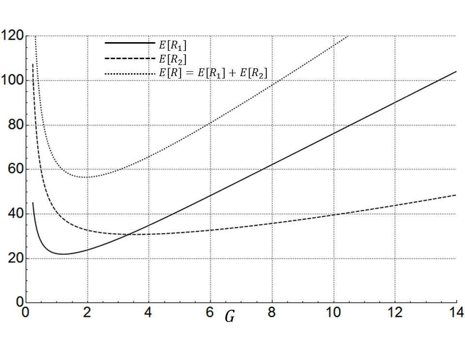
Figure 2: Mean number of customers vs length of glue period in case $G_{1}=G_{2}=G$.

Next we look in Fig 3 at the case where the glue periods $G_{1}$ and $G_{2}$ are unequal. In particular we look at the mean number of customers in the system of type-$1$, type-$2$ and in total if we vary one of the glue periods while keeping the other glue period constant.

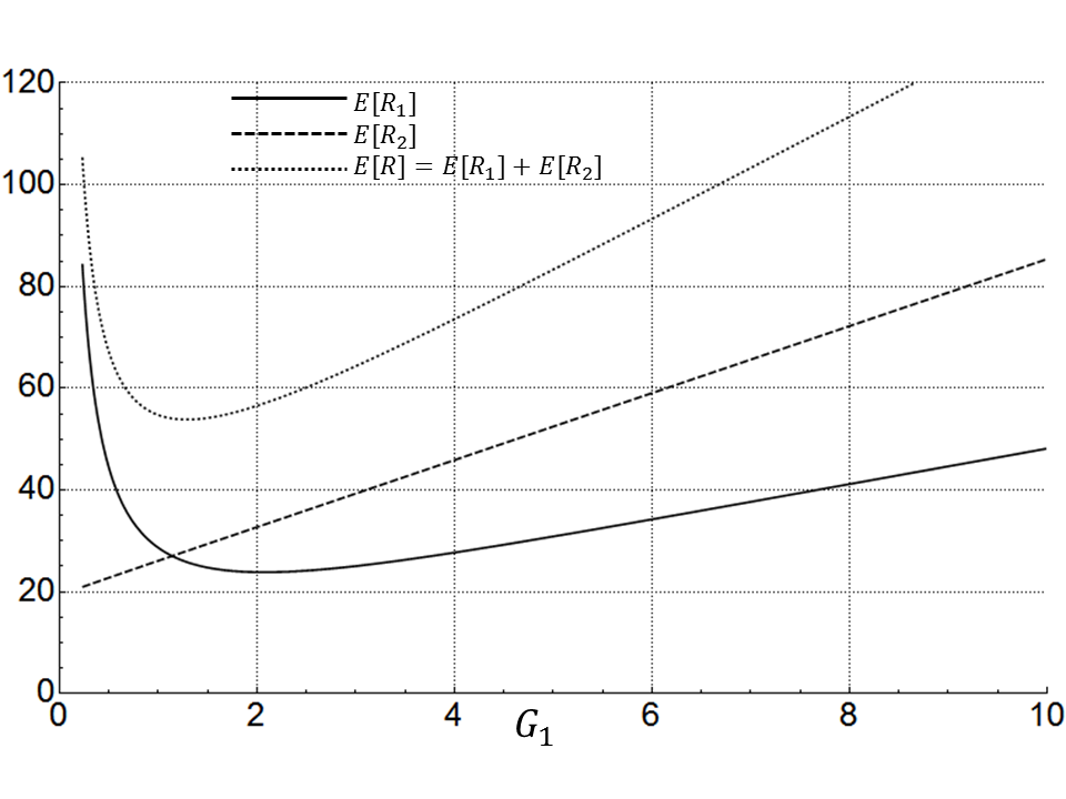
(a) varying $G_{1}$, with $G_{2}=2$

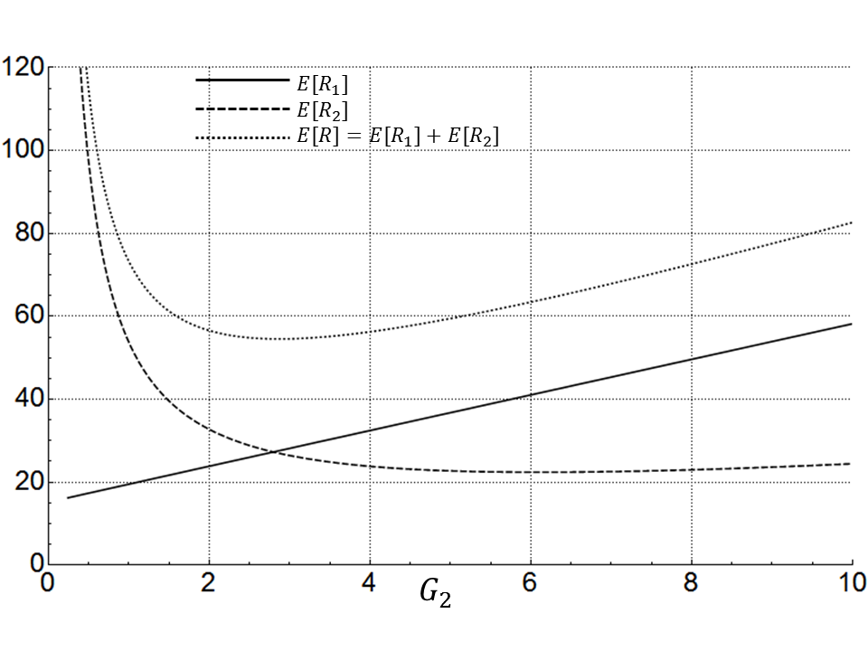
(b) varying $G_{2}$, with $G_{1}=2$

Figure 3: Mean number of customers vs length of glue period in case $G_{1}\neq G_{2}$.

The plots suggest that there is again a unique value of the length of the glue period that minimizes the mean total number of customers in the system. They also show that the length of the glue period that is optimal for $\mathbb{E}[R]$ is different from the one that is optimal for $\mathbb{E}[R_{1}]$ and the one that is optimal for $\mathbb{E}[R_{2}]$.

4 Conclusions and suggestions for future research

In this paper we have studied vacation queues and $N$-queue polling models with the gated service discipline and with retrials. Motivated by optical communications, we have introduced a glue period just before a server visit; during such a glue period, new customers and retrials "stick" instead of immediately going into orbit. For both the vacation queue and the $N$-queue polling model, we have derived steady-state queue length distributions at an arbitrary epoch and at various specific epochs. This was accomplished by establishing a relation to branching processes.

Jointly with B. Kim and J. Kim, in [1] we are considering the model with non-constant glue periods. We derive $\mathbb{E}[R]$ using MVA (mean value analysis) for the vacation model. It gives us the result for general glue period distributions without calculating the generating functions at different epochs. We show that a workload decomposition and pseudo conservation law, as discussed in [7] and Remark  7, can be derived for these variants and generalizations, and they may be exploited for analysis and optimization purposes. We shall then also try to explore the following observation: One may view our $N$-queue model as a polling model with a new variant of binomial gated, with adaptive probability $p_{i}$ of serving a customer at a visit of $Q_{i}$; $p_{i}=1$ when the customer arrived in the preceding glue period, and $p_{i}=1-{\rm e}^{-\nu_{i}G_{i}}$ otherwise. We would also like to explore the possibility to study the heavy traffic behavior of these models via the relation to branching processes, cf. [18].

From a more applied perspective we are looking into systems with multiple customer classes where one class has priority over another. This would help to incorporate the real life scenario where some type of data packets, like video buffering, should have as low latency as possible, whereas others, like a file transfer, can be delayed a bit longer.

Finally, we would like to point out an important advantage of optical fibre: the wavelength of light. A fibre-based network node may thus route incoming packets not only by switching in the time-domain, but also by wavelength division multiplexing. In queueing terms, this gives rise to multiserver polling models, each server representing a wavelength. We refer to [2] for the stability analysis of multiserver polling models, and to [3] for a mean field approximation of large passive optical networks. Therefore we would like to study multiserver polling models with the additional features of retrials and glue periods.

Acknowledgment

The authors gratefully acknowledge fruitful discussions with Kevin ten Braak and Tuan Phung-Duc about retrial queues and with Ton Koonen about optical networks. The research is supported by the IAP program BESTCOM, funded by the Belgian government, and by the Gravity program NETWORKS, funded by the Dutch government.

References

- [1] M.A. Abidini, O.J. Boxma, B. Kim, J. Kim and J.A.C. Resing (2015). Performance analysis of polling systems with retrials and glue periods. Paper in preparation.
- [2] N. Antunes, Chr. Fricker and J. Roberts (2011). Stability of multi-server polling system with server limits. Queueing Systems, 68, 229-235.
- [3] N. Antunes, Chr. Fricker, Ph. Robert and J. Roberts (2010). Traffic capacity of large WDM Passive Optical Networks. Proceedings 22nd International Teletraffic Congress (ITC 22), Amsterdam, September 2010.
- [4] J.R. Artalejo and A. Gomez-Corral (2008). Retrial Queueing Systems: A Computational Approach (Springer-Verlag, Berlin).
- [5] K.B. Athreya and P.E. Ney (1972). Branching Processes (Springer-Verlag, Berlin).
- [6] M.A.A. Boon, R.D. van der Mei, and E.M.M. Winands (2011). Applications of polling systems. SORMS, 16, 67-82.
- [7] O.J. Boxma (1989). Workloads and waiting times in single-server systems with multiple customer classes. Queueing Systems, 5, 185-214.
- [8] O.J. Boxma and J.W. Cohen (1991). The queue with permanent customers. IEEE J. Sel. Areas in Commun., 9, 179-184.
- [9] O.J. Boxma, O. Kella and K.M. Kosinski (2011). Queue lengths and workloads in polling systems. Operations Research Letters, 39, 401-405.
- [10] O.J. Boxma and J.A.C. Resing (2014). Vacation and polling models with retrials. 11th European Workshop on Performance Engineering (EPEW 11), Florence, September 2014.
- [11] G.I. Falin and J.G.C. Templeton (1997). Retrial Queues (Chapman and Hall, London).
- [12] C. Langaris (1997). A polling model with retrial of customers. Journal of the Operations Research Society of Japan, 40, 489-507.
- [13] C. Langaris (1999). Gated polling models with customers in orbit. Mathematical and Computer Modelling, 30, 171-187.
- [14] C. Langaris (1999). Markovian polling system with mixed service disciplines and retrial customers. Top, 7, 305-322.
- [15] H. Levy (1991). Binomial-gated service: A method for effective operation and optimization of polling systems. IEEE Trans. Commun., 39, 1341-1350.
- [16] H. Levy and M. Sidi (1990). Polling models: applications, modeling and optimization. IEEE Trans. Commun., 38, 1750-1760.
- [17] M. Maier (2008). Optical Switching Networks (Cambridge University Press, Cambridge).
- [18] R.D. van der Mei (2007). Towards a unifying theory on branching-type polling systems in heavy traffic. Queueing Systems, 57, 29-46.
- [19] Y. Okawachi, M.S. Bigelow, J.E. Sharping, Z. Zhu, A. Schweinsberg, D.J. Gauthier, R.W. Boyd and A.L. Gaeta (2005). Tunable all-optical delays via Brillouin slow light in an optical fiber. Physical Review Letters, 94, 153902.
- [20] M.P. Quine (1970). The multitype Galton-Watson process with immigration. Journal of Applied Probability 7, 411-422.
- [21] J.A.C. Resing (1993). Polling systems and multitype branching processes. Queueing Systems 13, 409-426.
- [22] W. Rogiest (2008). Stochastic Modeling of Optical Buffers. Ph.D. Thesis, Ghent University, Ghent, Belgium.
- [23] H. Takagi (1991). Application of polling models to computer networks. Comput. Netw. ISDN Syst., 22, 193-211.
- [24] H. Takagi (1991). Queueing Analysis: A Foundation of Performance Evaluation. Volume 1: Vacation and Priority Systems (Elsevier Science Publishers, Amsterdam).
- [25] H. Takagi (1997). Queueing analysis of polling models: progress in 1990-1994. In J.H. Dshalalow, editor, Frontiers in Queueing: Models, Methods and Problems, pages 119-146. CRC Press, Boca Raton, 1997.
- [26] H. Takagi (2000). Analysis and application of polling models. In G. Haring, C. Lindemann, and M. Reiser, editors, Performance Evaluation: Origins and Directions, volume 1769 of Lecture Notes in Computer Science, pages 424-442. Springer, Berlin, 2000.
- [27] N. Tian and Z.G. Zhang (2006). Vacation Queueing Models: Theory and Applications (Springer, New York).
- [28] V.M. Vishnevskii and O.V. Semenova (2006). Mathematical methods to study the polling systems. Autom. Remote Control, 67, 173-220.