Chaotic Explosions

Abstract

We investigate chaotic dynamical systems for which the intensity of trajectories might grow unlimited in time. We show that (i) the intensity grows exponentially in time and is distributed spatially according to a fractal measure with an information dimension smaller than that of the phase space, (ii) such exploding cases can be described by an operator formalism similar to the one applied to chaotic systems with absorption (decaying intensities), but (iii) the invariant quantities characterizing explosion and absorption are typically not directly related to each other, e.g., the decay rate and fractal dimensions of absorbing maps typically differ from the ones computed in the corresponding inverse (exploding) maps. We illustrate our general results through numerical simulation in the cardioid billiard mimicking a lasing optical cavity, and through analytical calculations in the baker map.

I Introduction

Fractality is a signature of chaos appearing in strange attractors and in the invariant sets of open dynamical systems Ott-book ; LaiTel-book ; GaspardBook . Here we are interested in systems in which trajectories have associated to them a time-varying intensity. In a recent work PRL we showed that fractality in chaotic systems in which the intensity of trajectories decays due to absorption can be described by an operator formalism and that absorption leads to a multi-fractal spectrum of the decaying state. In this work we investigate the dynamical and fractal properties of systems containing gain (i.e., negative absorption). In systems with gain the energy or intensity of trajectories increases in time, e.g., the intensity of a ray grows while it is in a gain medium or is multiplied by a factor larger than one when reflected on a wall.

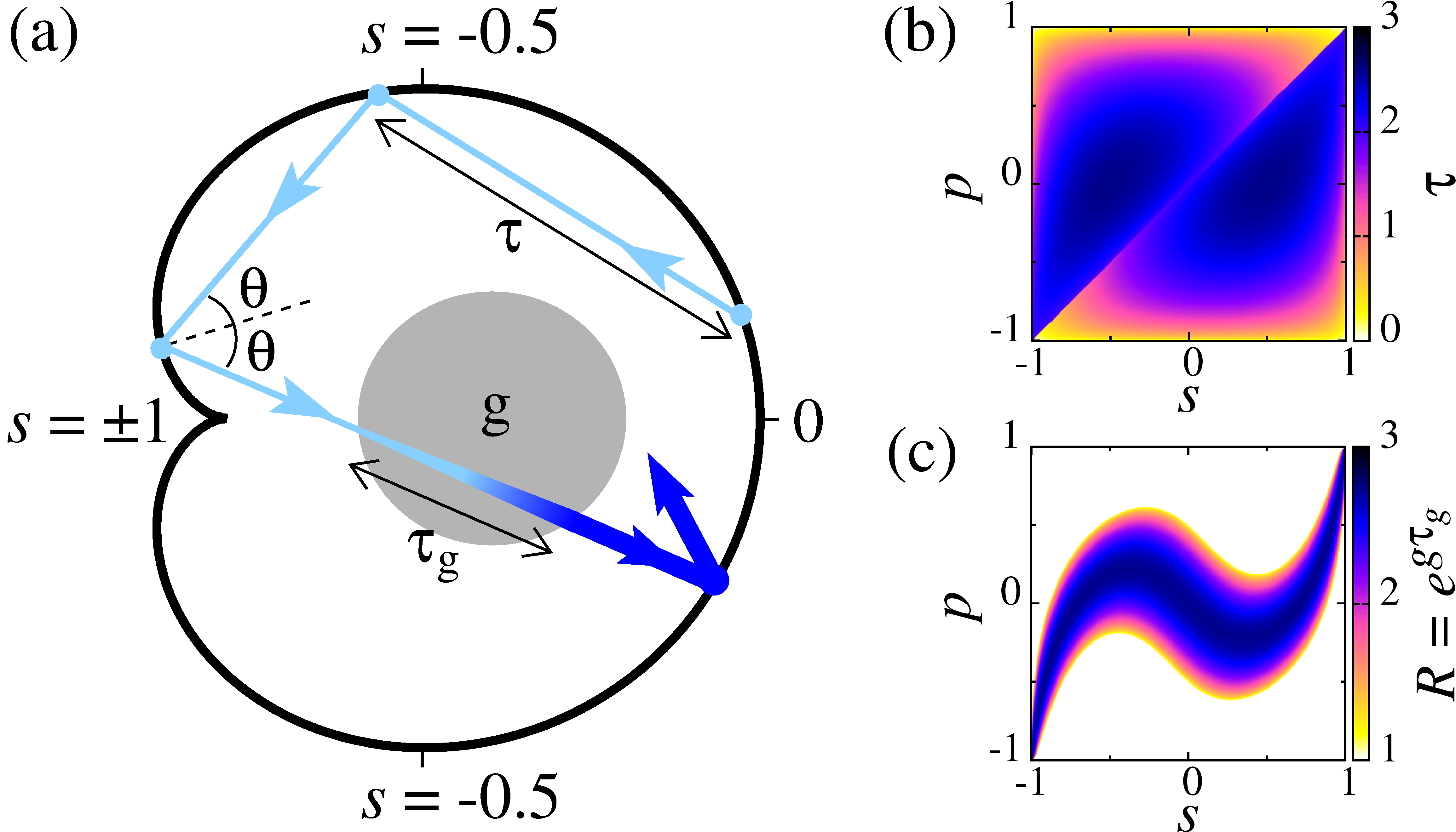
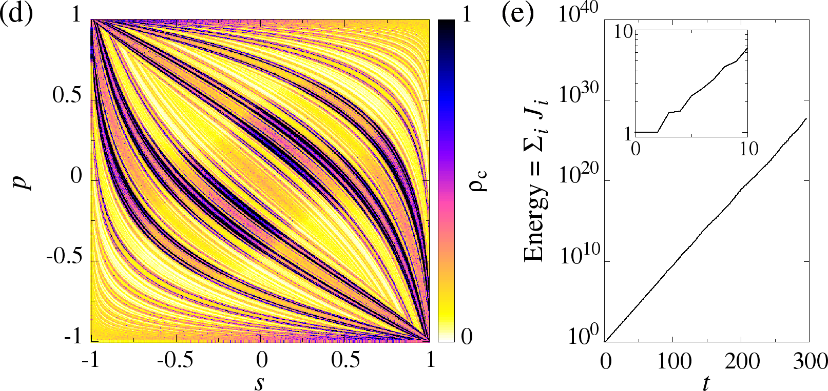
Figure 1: Explosion in a fully chaotic billiard. (a) Cardioid billiard, whose boundary in polar coordinates is $r(\phi)=1+\cos(\phi)$ with $\phi\in[-\pi,\pi]$ Robnik1983 . The gain region (gray, marked by g) is a disc of radius $0.5$ in the middle of the billiard. (b) Collision time distribution $\tau(\vec{x})$ in the cardioid billiard (velocity modulus is unity). Birkhoff coordinates $\vec{x}=(s,p=\sin\theta)$ are used, where $s$ is the arc length along the boundary and $\theta$ is the collision angle. (c) Reflection coefficient distribution: $R(\vec{x})=e^{g\tau_{g}}$ with $g=1$ and $\tau_{g}$ given by the length of the intersection of the ray with the gain region. (d) Time-independent density $\rho_{c}$ in the phase space. (e) Time-dependence of the intensity integrated over the phase space. The explosion rate $\kappa\approx 0.215$ is the slope of the curve (note the log-scale). Inset shows the non-exponential behavior for short times.

Optical microcavities provide a representative physical system of the general dynamical-systems picture described above. The formalism of open chaotic systems has been extensively used to describe lasing properties of two-dimensional optical cavities Harayama2011 ; RMP . The success of this approach relies on the use of long-living ray trajectories to describe the lasing modes. This is justified because lasing modes are induced by the gain medium present in optical cavities and only long-living trajectories are able to profit from this gain. The relevance of gain led to specific investigations of its role in experiments Shinohara2011 and wave simulations Martina2013 , but we are not aware of ray simulations which have explicitly included gain. This is a crucial issue especially when the gain is not uniformly distributed in the cavity, as in the experiments of Ref. Shinohara2011 .

We consider chaotic billiards with gain as models of optical microcavities. In Fig. 1 we show simulations of trajectories that bounce elastically, but whose intensities increase exponentially in time with rate $g$ while passing through a gain region (the gray disc in Fig. 1a). For long times, the total intensity grows exponentially in time and the spatial distribution (obtained for any $t$ normalizing over the phase space) approaches a fractal density $\rho_{c}$. We call this phenomenon a chaotic explosion.

In this Letter we show that chaotic systems with gain can be treated with the same formalism of systems with absorption but that the properties of these two classes of systems cannot be trivially related to each other. We obtain general results for the fractality and for the inverse map of systems with gain/absorption, which are illustrated analytically in the baker map and numerically in the cardioid billiard. For optical microcavities, our results show how gain can be introduced in the ray description and how it affects the far-field emission, demonstrating also in the ray description that lasing is not determined by the shape of the (passive) cavity alone.

II True-time maps with gain

We consider an extended map which includes, besides a usual map $f$, the true physical time $t_{n}$ and the ray intensity $J_{n}$ at the $n$-th intersection $\vec{x}_{n}$ with a Poincaré section as Gaspard1996 ; Kaufmann2001

$$f_{\text{ext}}:\left\{\begin{array}[]{lll}\vec{x}_{n+1}&=f(\vec{x}_{n}),\\ t_{n+1}&=t_{n}+\tau(\vec{x}_{n}),\\ J_{n+1}&=J_{n}R(\vec{x}_{n}),\end{array}\right.$$ (1)

where the return time $\tau(\vec{x})\geq 0$, chosen as the time between intersections $\vec{x}=\vec{x}_{n}$ and $\vec{x}_{n+1}=\vec{x}^{\prime}\equiv f(\vec{x})$ (for billiards, $\tau$ is the collision time between two consecutive bounces with the wall), and the reflection coefficient $R(\vec{x})$ are known functions of the coordinate $\vec{x}$ on the Poincaré section. Cases in which gain occurs continuously in time (not only at the intersection with the Poincaré section) correspond to a reflection coefficient $R(\vec{x})=e^{g\tau_{g}(\vec{x})}$, where $g$ is the gain rate and $\tau_{g}$ is the time spent in the gain region ($\tau_{g}=\tau$ if gain is uniform in the billiard table). Explosion occurs if $R(\vec{x})>1$ for a sufficiently large region of $\vec{x}$.

We are interested in the density $\rho(\vec{x},t)$ (i.e., the collective intensity of an ensemble of trajectories) at time $t$ in $\vec{x}$. Here we consider the class of (ergodic and chaotic) maps $f(\vec{x}_{n})$ for which we show that for any smooth initial $\rho(\vec{x},t=0)$ one observes for long times

$$\rho(\vec{x},t)\sim\rho_{c}(\vec{x})e^{\kappa t},$$ (2)

where $\kappa$ is the temporal rate of the total energy change (an explosion rate for $\kappa>0$) and is independent of $\rho(\vec{x},t=0)$.

We can expect that $\rho_{c}(\vec{x})$ of (2) is the attracting density of an iteration scheme for $\rho(\vec{x})$ of the extended map (1). With a compensation factor $e^{-\kappa\tau(\vec{x})}$ per iteration, this scheme evolves a density $\rho_{n}(\vec{x})$ at discrete time $n$ into $\rho_{n+1}(\vec{x})$ at the next intersection with the Poincaré surface of section as

$$\rho_{n+1}(\vec{x}^{\prime})=\sum_{\vec{x}\in{f}^{-1}({\vec{x}^{\prime})}}e^{-\kappa\tau(\vec{x})}\frac{R(\vec{x})\rho_{n}(\vec{x})}{\mid\mathcal{D}_{f}(\vec{x})\mid},$$ (3)

where $\mathcal{D}_{f}$ represents the Jacobian of the Poincaré map $f$. In the special case of invertible area-preserving dynamics (as in the billiard of Fig. 1), $\mathcal{D}_{f}(\vec{x})=1$ and there is no sum in (3) (map $f$ has a single preimage).

In any extended map, there exists one $\kappa$ – the one appearing in Eq. (2) – for which $\rho_{c}(\vec{x})$ arises as the limiting ($n\rightarrow\infty$) distribution of $\rho_{n}(\vec{x})$ iterated by scheme (3). The right-hand-side of Eq. (3), with the proper $\kappa$, is an operator with largest eigenvalue unity and $\rho_{c}$ as the corresponding eigenfunction. The second-largest eigenvalue controls the convergence of a smooth initial density $\rho_{0}$ to $\rho_{c}$. In agreement with the physical picture, we see that for extended maps $f_{\text{ext}}$ there are three different factors contributing to the density $\rho$: reflectivity $R$, return times $\tau$, and stretching of phase space volume $\mathcal{D}_{f}$. The rate $\kappa$ follows from the constraint that the compensated intensity neither increases nor decreases for large $n$ LaiTel-book .

Comparing with our previous results PRL ; RMP , we see that (3) is an extension to cases with $R>1$ of the Frobenius-Perron operator considered previously only in systems with absorption ($R\leq 1$ for any $\vec{x}$). The explosion rate $\kappa$ plays the role of a negative escape rate and the attracting limit distribution $\rho_{c}$ is the conditionally invariant density RMP (also known as the steady probability distribution in the optics community Lee2004 ; Ryu2006 ). By integrating, for $n\rightarrow\infty$, (3) over all $\vec{x}^{\prime}$, the left hand side is unity due to normalization of $\rho_{n}(\vec{x})$, while the right hand side is an average taken with respect to $\rho_{c}$. This yields (see also Ref. PRL ) $\langle e^{-\kappa\tau}R\rangle_{c}=1.$ For chaotic explosions this means that typically $R>1$, but its reduced value $e^{-\kappa\tau}R$ taken with the proper explosion rate averages out to unity if the average is taken with the $\rho_{c}$ associated to $\kappa$.

III General Features

It is remarkable that the formalism of transient chaos GaspardBook ; LaiTel-book can be applied with slight modifications to describe chaotic explosions. Below we use this formalism to explore the most interesting effects of gain ($R>1$).

III.1 Fractality

We first derive general relations between the fractality of $\rho_{c}$ – the eigenfunctions of Eq. (3) – and the distributions $(\tau(\vec{x}),R(\vec{x}))$ characterizing the extended map $f_{\text{ext}}$. Let us consider the map $f$ in (1) to be invertible and two-dimensional. We are interested in the dynamics within a region of interest $\Gamma$ only, which has a size of order unity in appropriately chosen units. Considering the $n$-th image and preimage of $\Gamma$ taken with the map $f$, we find for $n\gg 1$ a set of narrow “columns” in the unstable direction and narrow “strips” along the stable directions, as illustrated in Fig. 2. They are good approximants of the unstable and stable foliation of the chaotic set (a chaotic sea or an attractor in closed systems, or a chaotic saddle in open ones) underlying the dynamics. Each of them contains an element of an $n$-cycle Ott-book ; LaiTel-book , i.e., a point which is mapped by $f$ onto itself after $n$ iterations.

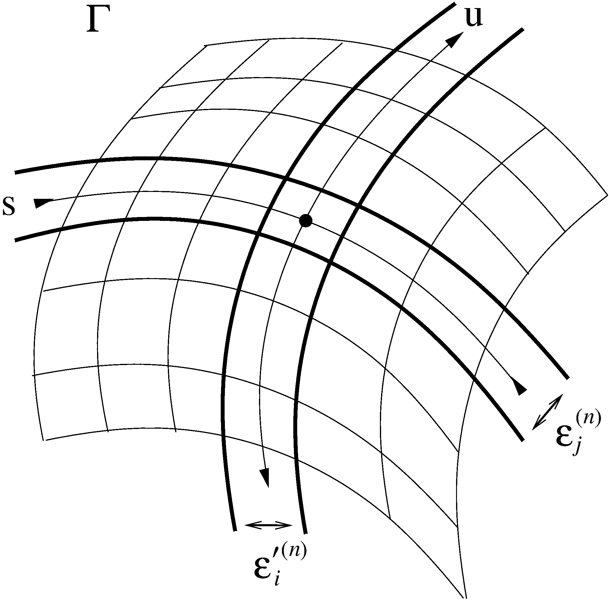
Figure 2: Schematic diagram of the phase-space partitioning around a hyperbolic chaotic set obtained taking the $n\gg 1$ fold image and preimage of the region of interest $\Gamma$ with respect to the (usual) map $f$. These define narrow strips and columns overlapping with branches of the stable (s) and unstable (u) manifold, respectively. The emphasized strip and column belong to a $n$-cycle point ($\bullet$) on the chaotic set.

Let us focus on such an $n$-cycle point at the intersection of strip $j$ and column $i$ (drawn with bold lines in Fig. 2). Due to the permanent contraction in the stable direction, the width of column $i$ is approximately $\varepsilon_{i}^{\prime(n)}=e^{{\lambda^{\prime}}_{i}^{(n)}n}$ where ${\lambda^{\prime}}_{i}^{(n)}<0$ is the contracting Lyapunov exponent around the cycle point over discrete time $n$. Similarly, the height $\varepsilon_{j}^{(n)}$ of strip $j$ is $\varepsilon_{j}^{(n)}=e^{-\lambda_{j}^{(n)}n}$, where $\lambda_{j}^{(n)}>0$ denotes the corresponding positive Lyapunov exponent. By construction, points starting in strip $j$ spend the dominant part of their lifetime $n$ in the close vicinity of the hyperbolic cycle in question (which belongs to the chaotic set). Therefore, for large $n$ nearly all points in the strip are subjected to an average stretching factor $e^{\lambda_{j}^{(n)}n}$ (in the unstable direction). In an extended map $f_{\text{ext}}$, obtained from $f$ through Eq. (1), these points experience an average collision time $\tau^{(n)}_{j}=\sum_{k=1}^{n}\tau_{k}/n$ and an average gain/reflection coefficient $R^{(n)}_{j}=(\Pi_{k=1}^{n}R_{k})^{1/n}$ while being around the $n$-cycle, where $\tau_{k}$ and $R_{k}$ denote the collision time and reflection coefficient, respectively, belonging to element $k$ of the $n$-cycle.

In the spirit of operator (3) valid for $f_{\text{ext}}$, the density on the images of strip $j$ is the density of strip $j$ multiplied (in each iteration) by a factor $R_{k}e^{-\kappa\tau_{k}}$. Starting with an initial unit density, the area $\varepsilon_{j}^{(n)}\times 1$ of strip $j$ should be multiplied in $f_{\text{ext}}$ by a factor $e^{-\kappa\tau^{(n)}_{j}n+n\ln{R^{(n)}_{j}}}$ by the end of $n$ iterations. Since the $n$-th image of strip $j$ with respect to $f$ is column $i$, by construction, the measure accumulating on column $i$ is

$$\mu^{(n)}_{i}=e^{-\kappa\tau^{(n)}_{j}n+n\ln{R^{(n)}_{j}}}\varepsilon^{(n)}_{j}=e^{\left(\ln{R^{(n)}_{j}}-\kappa\tau^{(n)}_{j}-\lambda_{j}^{(n)}\right)n}.$$ (4)

The existence of a time-independent measure implies that with the proper value of $\kappa$ we have $\sum_{i}\mu^{(n)}_{i}=1$.

In the spirit of dynamical systems theory, we associate with strip $j$ the measure that its points represent after $n$ steps. Therefore the measure $\mu^{(n)}_{j}$ of strip $j$ is

$$\mu^{(n)}_{j}=\mu^{(n)}_{i}.$$ (5)

The relation expresses that $f_{\text{ext}}$ maps the measures of the stable and unstable directions into each other.

We now focus on fractal properties of this measure. Systems described by closed maps $f$ with gain have a trivial fractal dimension $D_{0}$ equal to the phase space dimension. Their fractality requires thus the computation of the generalized dimensions Ott-book ; LaiTel-book

$$D_{q}=\frac{1}{1-q}\lim_{\varepsilon\rightarrow 0}\frac{\ln\sum_{k}\mu_{k}^{q}}{\ln 1/\varepsilon}$$ (6)

where $\mu_{k}$ is the measure of the $k$-th box in a coverage with a uniform grid of box size $\varepsilon$, and the sum is over non-empty boxes.

A general result can be obtained for the information dimension $D_{1}$. For a general one-dimensional distribution containing measures $\mu_{\alpha}$ in intervals of different sizes $\varepsilon_{\alpha}$ we have for small $\varepsilon_{\alpha}$ Ott-book ; LaiTel-book : $D_{1}=\sum_{\alpha}\mu_{\alpha}\ln{\mu_{\alpha}}/\sum_{\alpha}\mu_{\alpha}\ln{\varepsilon_{\alpha}}$. Now, take a section of strip $j$ along the unstable foliation (u), and associate the measure of the strip $\mu_{j}^{(n)}$ to the interval size $\varepsilon_{j}^{(n)}$. In the limit $n\gg 1$ the sizes are small, and substituting Eq. (4), (5) in the $D_{1}$ formula above, we obtain the partial information dimension $D^{(1)}_{1}$ along the unstable direction as

$$D^{(1)}_{1}=1+\frac{\kappa\bar{\tau}-\overline{\ln R}}{\bar{\lambda}}.$$ (7)

The averages denoted by overbars are taken over the chaotic set (e.g., $\bar{\lambda}$ is the positive Lyapunov exponent on the saddle). This is so because, as argued above, the trajectory effectively experiences collision times $\tau$, reflection coefficients $R$, and local Lyapunov exponents $\lambda$ (of the usual map $f$) close to an unstable cycle (which belongs to the chaotic set). Quantities characterizing the map ($\bar{\lambda}$), the collision times ($\bar{\tau}$), and the gain ($\overline{\ln R}$) determine a fractal property ($D_{1}$) via the simple relation (7). Fractality is nontrivial if $D^{(1)}_{1}<1$, implying $\kappa\bar{\tau}<\overline{\ln R}$ (for a positive rate $\kappa$), i.e., $R>1$ in a sufficiently extended region.

Repeating the calculation along a section parallel to the stable foliation (s) we find $D^{(2)}_{1}$, the partial information dimension along the stable direction. Since the measures are the same (see (5)), the difference follows from the sizes which are $\varepsilon_{i}^{{}^{\prime}(n)}$ now, and we find

$$D^{(2)}_{1}\mid\bar{\lambda^{\prime}}\mid=D^{(1)}_{1}\bar{\lambda}.$$ (8)

The overall information dimension of the chaotic set with the measure of $f_{\text{ext}}$ is $D_{1}=D^{(1)}_{1}+D^{(2)}_{1}$. The derivation above holds for any value of $R$ and therefore generalizes the results of Ref. PRL , where we conjectured Eq. (7) (with a negative $\kappa$) for strictly absorbing cases ($R\leq 1$). The case of usual maps ($\tau=1,R=1$) follows as a limit: if the map is closed (no loss in any sense), $\kappa=0$, and $D_{1}=1+\bar{\lambda}/\mid\bar{\lambda^{\prime}}\mid$, i.e. we recover the Kaplan-Yorke formula Ott-book ($D_{1}=2$ for area preserving maps); if the map is open (trajectories escape), $\kappa<0$, and Eqs. (7) and (8) go over into the Kantz-Grassberger formulas GaspardBook ; LaiTel-book .

III.2 Inverse map

Besides the physical motivation to study gain, a natural question that can only be answered considering both $R>1$ and $R<1$ is the one of the inverse of the extended map defined in Eq. (1), which we denote by $f^{\text{inv}}_{\text{ext}}$ and define implicitly by $f_{\text{ext}}\circ f^{\text{inv}}_{\text{ext}}=I,$ where $I$ is the identity. If $f_{\text{ext}}$ has $R>1$, then $f^{\text{inv}}_{\text{ext}}$ should compensate this with $R<1$.

For $f^{\text{inv}}_{\text{ext}}$ to exist, the usual map $f$ has to be invertible (i.e., $f$ must have a single pre-image). Consider the case in which the dynamics is defined in a bounded region, i.e., $f$ is closed. In this case the procedure for defining $f^{\text{inv}}_{\text{ext}}$ is to take $f^{-1}$ of the usual map $f$ and attribute to $x^{\prime}=f(x)$ the negative of the same return time $\tau^{\text{inv}}(x^{\prime})=-\tau(x)<0$ and the inverse reflection coefficient $R^{\text{inv}}(x^{\prime})=1/R(x)$. We can therefore write:

$$f^{\text{inv}}_{\text{ext}}:\left\{\begin{array}[]{lll}\vec{x}_{n+1}&=f^{\text{inv}}(\vec{x}_{n})&=f^{-1}(\vec{x}_{n}),\\ t_{n+1}&=t_{n}+\tau^{\text{inv}}(\vec{x}_{n})&=t_{n}-\tau(f^{-1}(\vec{x}_{n})),\\ J_{n+1}&=J_{n}R^{\text{inv}}(\vec{x}_{n})&=J_{n}/R(f^{-1}(\vec{x}_{n})).\end{array}\right.$$ (9)

The iteration corresponding to (3) of the inverted extended map in cases when $f$ describes a closed map is

$$\begin{array}[]{ll}\rho_{n+1}(\vec{x}^{\prime}\equiv{f}^{-1}({\vec{x})})&=e^{\kappa^{\text{inv}}\tau^{\text{inv}}(\vec{x})}\dfrac{R^{\text{inv}}(\vec{x})}{\mid\mathcal{D}^{\text{inv}}_{f}(\vec{x})\mid}\rho_{n}(\vec{x})\\ &=e^{-\kappa^{\text{inv}}\tau(\vec{x}^{\prime})}\dfrac{(1/R(\vec{x}^{\prime}))}{\mid 1/\mathcal{D}_{f}(\vec{x}^{\prime})\mid}\rho_{n}(\vec{x}).\end{array}$$ (10)

This equation is different from the operator of $f_{\text{ext}}$ in Eq. (3). Therefore, for extended maps the chaotic properties ($\kappa$, fractality, etc.) of maps $f_{\text{ext}}$ and $f_{\text{ext}}^{\text{inv}}$ typically differ. In particular, the rate $\kappa^{\text{inv}}$ of the inverse map is not $-\kappa$ (nor any simple function of $\kappa$)

The difference in the asymptotic rates $\kappa^{\text{inv}}\neq-\kappa$ seems to contradict the fact that, by definition, maps $f_{\text{ext}}$ and $f_{\text{ext}}^{\text{inv}}$ cancel each other, i.e., the gain and loss resulting from $n$ applications of one map is exactly compensated by $n$ applications of the other map (for arbitrarily large $n$). The solution of this apparent paradox is that the asymptotic densities of the forward $\rho_{c}$ and inverse $\rho_{c}^{\text{inv}}$ maps differ. Taking $\rho_{c}$ (or $\rho_{c}^{\text{inv}}$) as initial condition $\rho_{0}$, $\kappa^{\text{inv}}=-\kappa$. However, these are atypical $\rho_{0}$. Generic ones converge exponentially fast to the $\rho_{c}$ of the corresponding map.

Many systems of interest are not restricted to a bounded phase space $\Omega$, as considered above. For instance, in scattering systems one usually defines a bounded region $\Gamma$ of interest (which contains all periodic orbits and the chaotic saddle), but the dynamics is defined in the full phase space. In this case, the inverse map is defined as above in the whole space, with the same region of interest $\Gamma$ since the chaotic saddle is invariant. Another case of interest is the one of total absorption in a localized region, i.e., $R(\vec{x})=0$ for some $\vec{x}\in\Omega$ . In this case, the inverse map can be defined only as the limiting case of $R\rightarrow 0_{+}$.

III.3 Who wins?

In a general system both gain and absorption coexist and a natural question is whether decay or explosion is observed globally . This is a priori unclear because of the non-trivial nature of the asymptotic density $\rho_{c}(\vec{x})$. When half of the phase space has $R_{L}$ and the other half $R_{R}$ as reflection coefficients one would intuitively expect for an ergodic system that a steady state is found with $R_{L}R_{R}=1$. When taking the return times $\tau_{i}$ into account, intuition says that for $R_{L}R_{R}=1$ the behavior that dominates is the one associated with the half space characterized by smaller collision times (with more collisions per time unit). As shown below, these two intuitions are not generally correct.

A particularly interesting case is the one of energetic steady states when the total energy neither grows nor decreases in time ($\kappa=0$), in spite of local gains and losses. Situations with $\kappa\approx 0$ remain unchanged for long times and are thus easy to observe. In this case there is no need for any extraction of intensity and the corresponding iteration scheme is given by Eq. (3) without the term $e^{-\kappa\tau(\vec{x})}$, i.e., the usual Frobenius-Perron equation for closed systems (even if $f$ is open). The density $\rho_{c}$ is invariant (not conditionally invariant), does not depend explicitly on the return times $\tau$, and $D_{1}$ is given by (7) with $\kappa=0$. As shown below, this configuration leads to a fractal invariant density even for volume-preserving dynamics.

IV Examples

In this section we use specific systems to explore the general results reported above. First, we consider the analytically treatable closed area-preserving baker map defined in Fig. 3 Ott-book ; LaiTel-book . Initially $\rho_{0}\equiv 1$. In the next step, $\rho_{0}$ is multiplied by $R_{k}e^{-\kappa\tau_{k}}$, $k=1$ or $2$, leading to two vertical columns of width $1/2$ lying along the $x=0$ and $x=1$ lines. They carry measures $P_{1}$ and $P_{2}$ where

$$P_{k}=R_{k}e^{-\kappa\tau_{k}}/2,\;\;\;\;k=1,2.$$ (11)

The construction goes on in a self-similar way, and the condition that the measure after appropriate compensation remains bounded ($\rho_{c}$ is reached) corresponds to $(P_{1}+P_{2})^{n}=1$, even after $n\gg 1$ steps. We thus find as an equation specifying the explosion rate $\kappa$:

$$P_{1}+P_{2}=1.$$ (12)

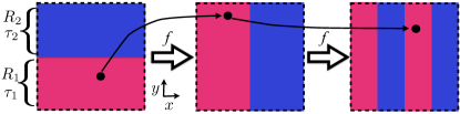
Figure 3: Action of the closed area-preserving baker map $f$ with gain on the unit square. The map $f$ is defined as $(x,y)^{\prime}=(x/2,2y)$ for $y<0.5$ and $(x,y)^{\prime}=(x/2+0.5,2y-1)$ for $y>0.5$ and extended – as in Eq. (1) – by assigning $R=R_{1}$ ($R=R_{2}$) and $\tau=\tau_{1}$ ($\tau=\tau_{2}$) to trajectories in the lower (upper) half.

IV.1 Fractality

The fractality of the baker map can be calculated explicitly. The generalized dimensions $D_{q}^{(2)}$ of $\rho_{c}$ along the stable (horizontal) direction is derived from Eqs. (6) and (11) as $D_{q}^{(2)}=\ln{(P_{1}^{q}+P_{2}^{q})}/[(1-q)\ln{2}].$ In the limit of $q\rightarrow 1$ the $D_{1}$ is obtained as

$$\begin{array}[]{ll}D_{1}^{(2)}&=1-[-\kappa\bar{\tau}+\overline{\ln R}]/\ln 2\\ &=1-\dfrac{-\kappa(\tau_{1}P_{1}+\tau_{2}P_{2})+P_{1}\ln{R_{1}}+P_{2}\ln{R_{2}}}{\ln 2},\end{array}$$ (13)

which is an equivalent derivation of the general formula (7) obtained by identifying $P_{i}$ with the measure on the chaotic set.

As a particular case, consider $\tau_{2}=2\tau_{1}\equiv 2\tau$ and $R_{1}=4,R_{2}=2$. From Eq. (12) a quadratic equation is obtained for $x\equiv e^{-\kappa\tau}>0$, leading to $x=\sqrt{2}-1$ and therefore a positive (explosion) rate $\kappa=-\ln{(\sqrt{2}-1)}/\tau\approx 0.881/\tau$ . Parameters $P_{1}$ and $P_{2}$ are then $2x$ and $x^{2}$, respectively. The average return time is $\bar{\tau}=\tau 2x+2\tau x^{2}=2\tau(2-\sqrt{2})$ while the average of $\ln{R}$ is found to be $(2\sqrt{2}-1)\ln{2}$. The numerator of the fraction in the parenthesis of Eq. (13) is $2(2-\sqrt{2})\ln{(\sqrt{2}-1)}+(2\sqrt{2}-1)\ln{2}\approx 0.235$. This is positive, rendering $D_{1}^{(2)}=1-0.235/\ln{2}\approx 0.616<D^{(2)}_{0}=1$, a clear sign of the multifractality of $\rho_{c}$.

IV.2 Inverse map

The inverse of the baker map discussed above is computed using the general relation (9). Symmetries and $\mathcal{D}_{f}=1$ make the inverse map to be equivalent (after a transformation $x\mapsto y,y\mapsto x$) to the forward map after replacing $R_{i}$ by $1/R_{i}$ and $\tau$ by $-\tau$ (see Fig. 3). In the example discussed above this corresponds thus to $\tau_{2}=2\tau_{1}=-2\tau,R_{1}=1/4$, $R_{2}=1/2$, which leads to $x\equiv e^{-\kappa\tau}=(\sqrt{65}-1)/4$. This is larger than $1$, implying a negative $\kappa^{\text{inv}}\approx-0.568/\tau$, i.e. an escape rate, a global decay of intensity towards zero. In Fig. 4 we confirm that these analytical calculations agree with simulations of individual trajectories. The different slopes confirm the general result $\mid\kappa\mid\neq\mid\kappa^{\text{inv}}\mid$. In the previous section we related this apparent paradox to the difference between $\rho_{c}$ and $\rho_{c}^{\text{inv}}$, which can be quantified by $D_{1}$. From Eq. (13), $D_{1}^{(2)\text{inv}}\approx 0.783\neq 0.661\approx D_{1}^{(2)}$. Non-trivial fractality is preserved despite the change of sign in $\kappa$.

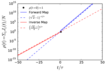
Figure 4: Explosion and escape rates $\kappa$ in the forward and inverse (extended) baker map. Points are distributed at $t=0$ uniformly in the phase space with $J_{i}=1$ and then iterated using Eq. (1) with $f$ defined in Fig. 3, $\tau_{2}=2\tau_{1}\equiv 2\tau$, and $R_{1}=4=2R_{2}$. The energy density $\rho(t)$ is computed as the average intensity of all trajectories $\rho=\sum_{i=1}^{N}J_{i}/N$ at time $t$. The forward map shows a growing energy in time ($t>0$, blue line) while the corresponding inverse map ($t<0$, red line) shows a decaying energy. Dashed lines are the analytical calculations.

IV.3 Who wins?

We allow for competition between gain and absorption in the particular example defined above by writing $R_{i}(\alpha)=\alpha R_{i}$, with $0<\alpha<1$. Because of (12), this leads with $R_{1}=4=2R_{2}$ to an $\alpha$-dependent explosion rate $\kappa(\alpha)$ given by $e^{-\kappa(\alpha)\tau}=\sqrt{1+1/\alpha}-1$. Decreasing $\alpha$ from unity, this quantity is less than unity but increases with decreasing $\alpha$. At $\alpha\lessapprox 1/2$ absorption and gain coexist ($R_{2}(\alpha)<1$) but explosion still dominates ($\kappa>0$). For $\alpha<\alpha_{c}=1/3$ absorption dominates ($\kappa<0$). At the critical value $\alpha=\alpha_{c}$, $\kappa=0$, which is the steady state condition, $R_{1c}\equiv R_{1}(\alpha=\alpha_{c})=4/3$, $R_{2c}\equiv R_{2}(\alpha=\alpha_{c})=2/3$, $P_{1c}=2/3$, $P_{2c}=1/3$, the average of $\ln{R}$ is $5/3\ln{2}-\ln{3}$, and thus Eq. (7) yields again fractality $D_{1}^{(2)}=1-\overline{\ln{R}}/\ln{2}=0.919$ for any $\tau_{1},\tau_{2}$.

Even though the return times $\tau_{i}$ are irrelevant at the steady state, the steady state is not achieved at $R_{1}R_{2}=1$. In our example, $R_{1}(\alpha)R_{2}(\alpha)=8\alpha^{2}=1$ for $\alpha=1/\sqrt{8}=0.354>\alpha_{c}=1/3$ (explosion). This remains valid in maps ($\tau_{i}=1$) for any $R_{1},R_{2}$: introducing $R_{1}=1/R_{2}$ in Eq. (12) leads to $\kappa\tau=\ln{((R_{1}+1/R_{1})/2)}\geq 0$. The stead-state condition is thus not $R_{1}R_{2}=1$, but rather $R_{1}+R_{2}=2$.

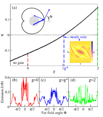
Figure 5: Ray emission from an optical cardioid billiard with gain and transmission. (a) Asymptotic rate $\kappa$ as a function of the gain strength $g$. The steady state $\kappa=0$ is achieved at $g=g^{*}\approx 1.0367$, the lower inset shows the invariant density $\rho_{c}$ for this case. (b-d) Long-time ($t\gg 1$) emission $E(\Phi)$ of intensity $J$ in the far-field angle $\Phi$ (normalized as $\int E(\Phi)d\Phi=1$) for (b) $g=0$, no gain and decaying intensity: $\kappa<0$; (c) $g=g^{*}$, steady state, $\kappa=0$; (d) $g=2$, explosion, $\kappa>0$. The intensity of rays grows with rate $g$ at the gain region (gray circle, see also Fig. 1) and is split between reflected and transmitted rays for small collision angles $\theta$. This leads to a partial optical reflection $R_{o}(\theta)=[\sin(\theta_{T}-\theta)/\sin(\theta_{T}+\theta)]^{2}<1$ for $\mid p\mid\equiv\mid\sin\theta\mid<1/\eta$, where we used $\eta=3$ and the transmitted angle $\theta_{T}$ is given by Snell’s law as $\eta\sin\theta=\sin\theta_{T}$ Lee2004 ; Ryu2006 .

As a final illustration of the significance of our general results, we perform numerical simulation of rays in an optical cavity with gain and absorption. Imagine that the cardioid billiard with localized gain introduced in Fig. 1 is composed of a dielectric material (with refraction index $\eta$). Figure 5 reports results for transverse-electric polarized light in such a configuration. Whether explosion occurs, depends on the gain parameter $g$ ($\kappa$ depends smoothly on $g$, see panel a). At the critical value $g=g*$ gain and loss cancel each other ($\kappa=0$) and an energetic steady state sets in. The density $\rho_{c}$ is fractal for any $g$, also at $g=g^{*}$ (see lower inset of panel a). The transmitted rays can be detected outside the billiard as an emission in a given direction (represented by the far-field angle $\Phi$, see upper inset in Fig. 5a). We obtain that the (observable) far-field emission (as a function of angle $\Phi$) is modified by the gain (compare panels b-d). We thus conclude that (non-uniform) gain has to be included in ray simulations.

V Conclusions

We considered chaotic systems in which the intensities of trajectories may grow in time (e.g., due to gain or a reflection coefficient $R>1$). We extended the formalism of systems with absorption ($R<1$) to show how the theory of (open) chaotic systems can be used in this new class of systems. For instance, we derived a formula – Eq. (7) – that relates the invariant properties (e.g., fractal dimensions and the explosion/escape rates) of systems with gain/absorption, a generalization of important results in the theory of open systems (in which $R$ is either $0$ or $1$) GaspardBook ; LaiTel-book . Despite the unifying formalism, our results reveal an intricate relationship between systems with gain and with absorption. For instance, the inverse of a system with gain is a system with absorption, but – in contrast to usual dynamical systems – their invariant properties are not trivially related to each other.

For applications in optical microcavities, our results show how gain can be incorporated in the usual ray simulations. Whenever the gain is not uniform in the cavity, we find that the emission is modified and can be described through our formalism of chaotic explosions. These results can be tested experimentally by constructing optical cavities with different localized gain regions Shinohara2011 and comparing the emission to ray simulations with and without gain.

VI Acknowledgments

We thank M. Schönwetter for the careful reading of the manuscript. This work has been supported by OTKA grant No. NK100296 and by the Alexander von Humboldt Foundation.

References

- (1) Ott E, Chaos in dynamical systems, Cambrdige Univ. Press, 1993.
- (2) Gaspard P, Chaos, Scattering and Statistical Mechanics, Cambridge Univ. Press, 2005.
- (3) Lai Y-C and Tél T, Transient Chaos: Complex Dynamics in Finite Time Scales, Springer, 2011.
- (4) Altmann E. G., Portela J. S. E., and Tél, T, Phys. Rev. Lett. 111, 144101 (2013).
- (5) Harayama T and Shinohara S, Laser Photonics Rev. 5, 247-271 (2011).
- (6) Altmann E. G., Portela J. S. E., and Tél, T, Rev. Mod. Phys. 85, 869–918 (2013).
- (7) Shinohara S, Harayama T, Fukushima T, Hentschel M, Sasaki T and Narimanov EE, Phys. Rev. A 83, 053837 (2011).
- (8) Kwon T-Y, Lee S-Y, Ryu J-W and Hentschel M, Phys. Rev. A 88, 023855 (2013).
- (9) Robnik M, J. Phys. A: Math. Gen. 16, 3971 (1983).
- (10) Gaspard P, Phys. Rev. E 53, 4379 (1996).
- (11) Kaufmann Z and Lustfeld H, Phys. Rev. E 64, 055206 (2001).
- (12) Lee S-Y, Rim S, Ryu J-W, Kwon, T-Y, Choi M, and Kim C-M, Phys. Rev. Lett. 93 13 (2004).
- (13) Ryu J-W, Lee S-Y, Kim C-M, and Park Y-J, Phys. Rev. E 73, 036207 (2011).