A Priori Error Analysis of Space–Time Trefftz Discontinuous Galerkin Methods for Wave Problems

Abstract

We present and analyse a space–time discontinuous Galerkin method for wave propagation problems. The special feature of the scheme is that it is a Trefftz method, namely that trial and test functions are solution of the partial differential equation to be discretised in each element of the (space–time) mesh. The method considered is a modification of the discontinuous Galerkin schemes of Kretzschmar et al. [25] and of Monk and Richter [28]. For Maxwell’s equations in one space dimension, we prove stability of the method, quasi-optimality, best approximation estimates for polynomial Trefftz spaces and (fully explicit) error bounds with high order in the meshwidth and in the polynomial degree. The analysis framework also applies to scalar wave problems and Maxwell’s equations in higher space dimensions. Some numerical experiments demonstrate the theoretical results proved and the faster convergence compared to the non-Trefftz version of the scheme.

Keywords:  Discontinuous Galerkin method, Trefftz method, space–time finite elements, wave propagation, Maxwell equations, a priori error analysis, approximation estimates.

AMS subject classification:  65M60, 65M15, 41A10, 41A25, 35Q61.

1 Introduction

In this paper we analyse the Trefftz discontinuous Galerkin (Trefftz-DG) finite element method for the space–time discretisation of time-dependent wave propagation problems.

Space–time finite element approximations of time-dependent wave problems constitute a viable alternative to methods based on finite element discretisations in space combined with time-stepping schemes. They provide a setting where high-order approximation in both space and time is obtained by simply increasing the order of the basis functions, spectral convergence of the error in the space–time domain can be achieved by $p$-refinement, and the $hp$-refinement techniques developed for spatial discretisations can be directly imported to space–time meshes and polynomial spaces. In particular, when local mesh refinement in space–time is implemented, the smallest space elements do not put constraints on the CFL condition in the rest of the domain. Space–time finite elements with continuous space discretisations were introduced in [21, 22, 13, 12, 33, 24] (several references to earlier works can be found in [22]); space–time DG methods have been studied in [10, 28, 34, 5, 26, 16].

In order to reduce the number of degrees of freedom needed to obtain a given accuracy, the space–time DG approach can be combined with the use of Trefftz approximating spaces, namely discrete spaces whose elements are piecewise solutions of the equation to be discretised.

While the literature on Trefftz finite elements for time-harmonic wave propagation problems is nowadays quite developed (see e.g. [4, 29, 32, 11, 14, 23, 6] for different approaches using Trefftz-type basis functions and e.g. [2, 15, 19, 20] for theoretical analyses), Trefftz methods for time-dependent wave problems are relatively new. For time-dependent scalar wave problems, a global Trefftz approach was first introduced in [27]. Space–time Trefftz methods enforcing the continuity constraints by Lagrange multipliers have been designed, based on the second order in time formulation [30, 35], while a Trefftz-DG method has been introduced in [25] for the electromagnetic wave problem in the one-dimensional spatial case and extended in [8] to the multidimensional case and to transparent boundary conditions. Numerical tests have shown that these methods actually deliver high-order space–time convergence, but no theoretical analysis was available.

Here, we focus on the discontinuous Galerkin approach, and we aim at developing an error analysis of space–time Trefftz-DG methods, based upon the framework developed in [19] for time-harmonic wave problems.

Following [25], the model problems we consider are the time-dependent Maxwell equations in one space dimension, with piecewise constant material coefficients and with either Dirichlet or Robin boundary conditions; they also cover the case of 1D scalar wave problems formulated as a first order system (see Remark 2.1). We prove that the Trefftz-DG method is well-posed and quasi-optimal, as its bilinear form is coercive and continuous in a DG norm, that the $L^{2}$ norm of the error is controlled, and that the scheme is dissipative. Since the Trefftz-DG method we consider is not of interior penalty type, no inverse estimates are needed, thus our scheme and its analysis also work with non-polynomial Trefftz approximations. The analysis framework of section 4 immediately extends to both scalar wave problems and Maxwell’s equations in higher space dimensions, see Remark 3.4. What is specific to the 1D spatial case, instead, are the best approximation properties of space–time Trefftz finite element spaces, and therefore the error convergence rates (see sections 5 and 6).

For the case of polynomial approximations, we prove that the Trefftz-DG method has a much better asymptotic behaviour in terms of accuracy per number of degrees of freedom, for both the $h$- and the $p$-versions, than standard methods using full polynomial discrete spaces. The approximation bounds for Trefftz spaces and those for full polynomial spaces have the same order $h^{p+1}$, with $h$ the meshsize and $p$ the polynomial degree, but a local full polynomial space of degree $p$ for the approximation of $(E,H)$ has dimension $(p+1)(p+2)={\mathcal{O}}(p^{2})$, while the corresponding Trefftz space has only dimension $2p+2={\mathcal{O}}(p)$. The constants in the final error bounds for the Trefftz-DG method (see Theorem 6.2) are completely explicit. A further advantage of the use of a Trefftz method is that its variational formulation only involves integrals on the skeleton of the space–time mesh, thus avoiding the computational burden of the calculation of volume integrals. We also present some numerical tests confirming these theoretical results, highlighting the faster convergence (both in the meshwidth and in the polynomial degree) compared to the non-Trefftz version of the method, and the mild dependence of the numerical error on the flux stabilisation parameters, which we introduce for analysis purposes.

The article is structured as follows. In section 2 we introduce the initial boundary value problems to be discretised and in section 3 we describe the DG formulation and its Trefftz version. In section 4 we prove the well-posedness of the Trefftz-DG method and the a priori error bounds in DG and $L^{2}$ norms. In section 5 we define local polynomial Trefftz spaces and prove best approximation estimates in anisotropic space–time Sobolev norms and in section 6 we combine the previous results into $hp$-error bounds for the Trefftz-DG scheme. Finally, in section 7 we show the results of some numerical experiments and in section 8 we outline some possible extensions of the scheme and of its analysis. Appendix A contains a different proof of the stability bound needed to control the $L^{2}$ norm of the error; this proof gives a better constant than that in section 4.2 but holds only for constant coefficients.

2 Model problems

In this section, we introduce the model problems we are going to consider in the rest of this paper, namely the time-dependent Maxwell equations in one space dimension, with either perfectly electrically conducting or absorbing boundary conditions. We refer to Remark 3.4 below for the three-dimensional case, while the case of the acoustic wave problem is discussed in Remark 2.1 (in one space dimension) and again in Remark 3.4 (in any space dimension).

Given a space domain $\Omega=(x_{L},x_{R})$ and a time domain $I=(0,T)$, we set $Q:=\Omega\times I$. We denote by ${{\mathbf{n}}}_{Q}=(n_{Q}^{x},n_{Q}^{t})$ the outward pointing unit normal vector on $\partial Q$.

We assume the electric permittivity ${\varepsilon}={\varepsilon}(x)$ and the magnetic permeability $\mu=\mu(x)$ to satisfy ${\varepsilon}(x)\geq{\varepsilon}_{*}>0$, $\mu(x)\geq\mu_{*}>0$, and to be piecewise constant in $\Omega$. The speed of light in the material is $c(x):=({\varepsilon}(x)\mu(x))^{-1/2}$.

We consider the Maxwell equations for an electromagnetic wave propagating along the direction $x$, in terms of the one-component electric and magnetic fields $E=E_{y}$ and $H=H_{z}$, respectively.

In the case of Dirichlet boundary conditions, the corresponding initial boundary value problem reads as

$$\begin{aligned} &\frac{\partial E}{\partial x}+\frac{\partial(\mu H)}{\partial t}=0&&\;\text{in}\;Q,\\ &\frac{\partial H}{\partial x}+\frac{\partial({\varepsilon}E)}{\partial t}=J&&\;\text{in}\;Q,\\ &E(\cdot,0)=E_{0},\quad H(\cdot,0)=H_{0}&&\;\text{on}\;\Omega,\\ &E(x_{L},\cdot)=E_{L},\quad E(x_{R},\cdot)=E_{R}&&\;\text{on}\;I,\end{aligned}$$ (1)

assuming sufficiently regular data $J,E_{0},H_{0},E_{L},E_{R}$. The case $E_{L}=E_{R}=0$ models a perfectly electric conductor.

We also consider the case of absorbing (Robin) boundary conditions:

$$\begin{aligned} &\frac{\partial E}{\partial x}+\frac{\partial(\mu H)}{\partial t}=0&&\;\text{in}\;Q,\\ &\frac{\partial H}{\partial x}+\frac{\partial({\varepsilon}E)}{\partial t}=J&&\;\text{in}\;Q,\\ &E(\cdot,0)=E_{0},\quad H(\cdot,0)=H_{0}&&\;\text{on}\;\Omega,\\ &{\varepsilon}^{1/2}E(x_{L},\cdot)+\mu^{1/2}H(x_{L},\cdot)=g_{L}&&\;\text{on}\;I,\\ &{\varepsilon}^{1/2}E(x_{R},\cdot)-\mu^{1/2}H(x_{R},\cdot)=g_{R}&&\;\text{on}\;I.\end{aligned}$$ (2)

Remark 2.1.

The case of the scalar wave equation in one space dimension

$$\frac{\partial{}^{2}U}{\partial t^{2}}-c^{2}\frac{\partial{}^{2}U}{\partial x^{2}}=c^{2}J$$ (3)

can be traced back to either (1) or (2) by setting

$$E=\frac{\partial U}{\partial t},\quad H=-\frac{\partial U}{\partial x}\quad\text{and}\quad\mu=1,$$

(where $c^{2}=1/{\varepsilon}\mu$ as above). The Dirichlet boundary conditions become $\frac{\partial U}{\partial t}(x_{L},\cdot)=E_{L}$ and $\frac{\partial U}{\partial t}(x_{R},\cdot)=E_{R}$. The absorbing boundary conditions become ${\varepsilon}^{1/2}\frac{\partial U}{\partial t}+\mu^{1/2}\frac{\partial U}{\partial x}=g_{L}$, ${\varepsilon}^{1/2}\frac{\partial U}{\partial t}-\mu^{1/2}\frac{\partial U}{\partial x}=g_{R}$.

In the following, we introduce the space–time Trefftz-DG method and develop its analysis in the case of the initial boundary value problem with Dirichlet boundary conditions (1). We address the case of the problem with Robin boundary conditions (2) in section 4.4 and in Remarks 6.4 and 6.5.

3 Space–time DG discretisation

Let $K\subset Q$ be a Lipschitz subdomain such that ${\varepsilon}$ and $\mu$ are constant in $K$; we denote by ${{\mathbf{n}}}_{K}=(n_{K}^{x},n_{K}^{t})$ the outward pointing unit normal vector on $\partial K$. Assume $E,H\in H^{1}(K)$. Multiplying the first and the second equation of (1) by the test functions $v_{H},v_{E}\in H^{1}(K)$ respectively, and integrating by parts we obtain

$$-\iint_{K} \Big{(}E\frac{\partial v_{H}}{\partial x}+\mu H\frac{\partial v_{H}}{\partial t}+H\frac{\partial v_{E}}{\partial x}+{\varepsilon}E\frac{\partial v_{E}}{\partial t}\Big{)}\,\mathrm{d}x\,\mathrm{d}t$$

$$+\int_{\partial K}\Big{(}(Ev_{H}+Hv_{E})n^{x}_{K}+(\mu Hv_{H}+{\varepsilon}Ev_{E})n^{t}_{K}\Big{)}\,\mathrm{d}s=\iint_{K}Jv_{H}\,\mathrm{d}x\,\mathrm{d}t.$$

(Here and in the following we omit writing the trace operator $\mathrm{Tr}:H^{1}(K)\to L^{2}(\partial K)$.)

3.1 Mesh and DG notation

We introduce a mesh ${\mathcal{T}}_{h}$ on $Q$, such that its elements are rectangles with sides parallel to the space and time axes, and all the discontinuities of the parameters ${\varepsilon}$ and $\mu$ lie on interelement boundaries (note that the method described in this paper can be generalised to allow discontinuities lying inside the elements as in [25]). The mesh may have hanging nodes.

We denote with ${\mathcal{F}}_{h}=\bigcup_{K\in{\mathcal{T}}_{h}}\partial K$ the mesh skeleton and its subsets:

$${{\mathcal{F}}_{h}^{\text{hor}}} :=\text{the union of the internal horizontal element sides ($t=$ constant)},$$

$${{\mathcal{F}}_{h}^{\text{ver}}} :=\text{the union of the internal vertical element sides ($x=$ constant)},$$

$${{\mathcal{F}}_{h}^{0}} :=[x_{L},x_{R}]\times\{0\},$$

$${{\mathcal{F}}_{h}^{T}} :=[x_{L},x_{R}]\times\{T\},$$

$${{\mathcal{F}}_{h}^{L}} :=\{x_{L}\}\times[0,T],$$

$${{\mathcal{F}}_{h}^{R}} :=\{x_{R}\}\times[0,T].$$

We define the following broken Sobolev space:

$$H^{1}({\mathcal{T}}_{h}):=\big{\{}v\in L^{2}(Q),\;v|_{K}\in H^{1}(K)\;\forall K\in{\mathcal{T}}_{h}\big{\}}$$

and the averages and jumps of functions $\phi\in H^{1}({\mathcal{T}}_{h})$:

$$\{\!\!\{\phi\}\!\!\} :=\frac{1}{2}\big{(}\phi_{|_{K_{1}}}+\phi_{|_{K_{2}}}\big{)} \;\text{on}\;(\partial K_{1}\cap\partial K_{2})\subset{{\mathcal{F}}_{h}^{\text{ver}}},$$

$$[\![\phi]\!]_{x} :=\phi_{|_{K_{1}}}n_{K_{1}}^{x}+\phi_{|_{K_{2}}}n_{K_{2}}^{x} \;\text{on}\;(\partial K_{1}\cap\partial K_{2})\subset{{\mathcal{F}}_{h}^{\text{ver}}},$$

$$[\![\phi]\!]_{t} :=\phi_{|_{K_{1}}}n_{K_{1}}^{t}+\phi_{|_{K_{2}}}n_{K_{2}}^{t} \;\text{on}\;(\partial K_{1}\cap\partial K_{2})\subset{{\mathcal{F}}_{h}^{\text{hor}}}.$$

We note that $[\![\phi]\!]_{x}$ is the trace of $\phi$ from the left minus that from the right; $[\![\phi]\!]_{t}$ is the trace from lower times minus that from higher times. On ${{\mathcal{F}}_{h}^{\text{hor}}}$, we denote by $\phi^{-}$ the trace of $\phi\in H^{1}({\mathcal{T}}_{h})$ taken from the adjacent element with lower time.

3.2 DG formulation

We introduce a (vector) finite dimensional subspace ${{\mathbf{V}}}_{p}({\mathcal{T}}_{h})\subset H^{1}({\mathcal{T}}_{h})^{2}$. The space–time DG discretisation of the initial-boundary value problem (1) consists in finding $(E_{hp},H_{hp})\in{{\mathbf{V}}}_{p}({\mathcal{T}}_{h})$ such that, for all $K\in{\mathcal{T}}_{h}$ and for all $(v_{E},v_{H})\in{{\mathbf{V}}}_{p}({\mathcal{T}}_{h})$, it holds

$$-\iint_{K} \Big{(}E_{hp}\frac{\partial v_{H}}{\partial x}+\mu H_{hp}\frac{\partial v_{H}}{\partial t}+H_{hp}\frac{\partial v_{E}}{\partial x}+{\varepsilon}E_{hp}\frac{\partial v_{E}}{\partial t}\Big{)}\,\mathrm{d}x\,\mathrm{d}t$$

$$+\int_{\partial K}\Big{(}(\widehat{E}_{hp}v_{H}+\widehat{H}_{hp}v_{E})n^{x}_{K}+({\varepsilon}\widehat{E}_{hp}v_{E}+\mu\widehat{H}_{hp}v_{H})n^{t}_{K}\Big{)}\,\mathrm{d}s=\iint_{K}Jv_{H}\,\mathrm{d}x\,\mathrm{d}t.$$ (4)

The numerical fluxes $\widehat{E}_{hp}$ and $\widehat{H}_{hp}$ are defined on the mesh skeleton ${\mathcal{F}}_{h}$ as

$$\widehat{E}_{hp}:=\begin{cases}E_{hp}^{-}&\;\text{on}\;{{\mathcal{F}}_{h}^{\text{hor}}},\\ E_{hp}&\;\text{on}\;{{\mathcal{F}}_{h}^{T}},\\ E_{0}&\;\text{on}\;{{\mathcal{F}}_{h}^{0}},\\ \{\!\!\{E_{hp}\}\!\!\}+\beta[\![H_{hp}]\!]_{x}&\;\text{on}\;{{\mathcal{F}}_{h}^{\text{ver}}},\\ E_{L}&\;\text{on}\;{{\mathcal{F}}_{h}^{L}},\\ E_{R}&\;\text{on}\;{{\mathcal{F}}_{h}^{R}},\end{cases}\qquad\widehat{H}_{hp}:=\begin{cases}H_{hp}^{-}&\;\text{on}\;{{\mathcal{F}}_{h}^{\text{hor}}},\\ H_{hp}&\;\text{on}\;{{\mathcal{F}}_{h}^{T}},\\ H_{0}&\;\text{on}\;{{\mathcal{F}}_{h}^{0}},\\ \{\!\!\{H_{hp}\}\!\!\}+\alpha[\![E_{hp}]\!]_{x}&\;\text{on}\;{{\mathcal{F}}_{h}^{\text{ver}}},\\ H_{hp}-\alpha(E_{hp}-E_{L})&\;\text{on}\;{{\mathcal{F}}_{h}^{L}},\\ H_{hp}+\alpha(E_{hp}-E_{R})&\;\text{on}\;{{\mathcal{F}}_{h}^{R}},\end{cases}$$ (5)

where $\alpha\in L^{\infty}({{\mathcal{F}}_{h}^{\text{ver}}}\cup{{\mathcal{F}}_{h}^{L}}\cup{{\mathcal{F}}_{h}^{R}})$ and $\beta\in L^{\infty}({{\mathcal{F}}_{h}^{\text{ver}}})$ are two positive flux parameters. The fluxes are chosen as upwind fluxes on horizontal mesh edges, and centred fluxes with the addition of a penalty jump stabilisation on vertical edges; other choices are possible.

Summing (4) over all the elements $K\in{\mathcal{T}}_{h}$, we obtain the variational formulation

$$\text{seek}\;(E_{hp},H_{hp})\in{{\mathbf{V}}}_{p}({\mathcal{T}}_{h})\;\text{such that}$$

$$a_{DG}(E_{hp},H_{hp};v_{E},v_{H})=\ell_{DG}(v_{E},v_{H})\qquad\forall(v_{E},v_{H})\in{{\mathbf{V}}}_{p}({\mathcal{T}}_{h}),$$ (6)

where

$$\begin{aligned} a_{DG}(E_{hp},H_{hp};&v_{E},v_{H}):=-\sum_{K\in{\mathcal{T}}_{h}}\iint_{K}\Big{(}E_{hp}\frac{\partial v_{H}}{\partial x}+\mu H_{hp}\frac{\partial v_{H}}{\partial t}+H_{hp}\frac{\partial v_{E}}{\partial x}+{\varepsilon}E_{hp}\frac{\partial v_{E}}{\partial t}\Big{)}\,\mathrm{d}x\,\mathrm{d}t\\ &+\int_{{{\mathcal{F}}_{h}^{\text{hor}}}}({\varepsilon}E_{hp}^{-}[\![v_{E}]\!]_{t}+\mu H_{hp}^{-}[\![v_{H}]\!]_{t})\,\mathrm{d}x+\int_{{\mathcal{F}}_{h}^{T}}({\varepsilon}E_{hp}v_{E}+\mu H_{hp}v_{H})\,\mathrm{d}x\\ &+\int_{{\mathcal{F}}_{h}^{\text{ver}}}\big{(}\{\!\!\{E_{hp}\}\!\!\}[\![v_{H}]\!]_{x}+\{\!\!\{H_{hp}\}\!\!\}[\![v_{E}]\!]_{x}+\alpha[\![E_{hp}]\!]_{x}[\![v_{E}]\!]_{x}+\beta[\![H_{hp}]\!]_{x}[\![v_{H}]\!]_{x}\big{)}\,\mathrm{d}t\\ &+\int_{{\mathcal{F}}_{h}^{L}}\big{(}-H_{hp}v_{E}+\alpha E_{hp}v_{E}\big{)}\,\mathrm{d}t+\int_{{\mathcal{F}}_{h}^{R}}\big{(}H_{hp}v_{E}+\alpha E_{hp}v_{E}\big{)}\,\mathrm{d}t,\end{aligned}$$ (7)

$$\begin{aligned} \ell_{DG}(v_{E},v_{H}):=&\iint_{Q}Jv_{H}\,\mathrm{d}x\,\mathrm{d}t+\int_{{\mathcal{F}}_{h}^{0}}({\varepsilon}E_{0}v_{E}+\mu H_{0}v_{H})\,\mathrm{d}x\\ &+\int_{{\mathcal{F}}_{h}^{L}}E_{L}(v_{H}+\alpha v_{E})\,\mathrm{d}t+\int_{{\mathcal{F}}_{h}^{R}}E_{R}(-v_{H}+\alpha v_{E})\,\mathrm{d}t.\end{aligned}$$

Remark 3.1.

In [28], a space–time DG discretisation of linear hyperbolic systems in $N$ dimensions is introduced. The formulation (6) with $\alpha=\beta=\frac{1}{2}$ and ${{\mathbf{V}}}_{p}({\mathcal{T}}_{h})=\mathbb{P}^{p}({\mathcal{T}}_{h})^{2}$, the space of piecewise polynomials of degree at most $p$ on ${\mathcal{T}}_{h}$, is a particular case of that of [28]. More precisely, in the notation of [28], assume the initial boundary value problem to be posed in one space dimension ($N=1$), and to have a linear hyperbolic system of dimension $m=2$ with time derivative coefficient matrix $A=(\begin{smallmatrix}1&0\\ 0&1\end{smallmatrix})$, and space derivative coefficient matrix $A_{1}=(\begin{smallmatrix}0&1\\ 1&0\end{smallmatrix})$. The solution will be the vector field ${{\mathbf{u}}}=(E,H)$. The matrix defining the Dirichlet boundary conditions takes values $\mathsf{N}|_{{{\mathcal{F}}_{h}^{L}}}=(\begin{smallmatrix}2&-1\\ 1&0\end{smallmatrix})$ and $\mathsf{N}|_{{{\mathcal{F}}_{h}^{R}}}=(\begin{smallmatrix}2&1\\ -1&0\end{smallmatrix})$, and the space–time mesh is taken as a Cartesian mesh aligned with the space and time axes. The numerical fluxes are defined through the following splitting of the matrix $\mathsf{M}=\left(\begin{smallmatrix}n^{t}_{K}&n^{x}_{K}\\ n^{x}_{K}&n^{t}_{K}\end{smallmatrix}\right)$: on the part of $\partial K$ with $n^{x}_{K}=1$, $\mathsf{M}_{+}=\frac{1}{2}(\begin{smallmatrix}1&1\\ 1&1\end{smallmatrix})$, $\mathsf{M}_{-}=\frac{1}{2}(\begin{smallmatrix}-1&1\\ 1&-1\end{smallmatrix})$, while on the part of $\partial K$ with $n^{x}_{K}=-1$, $\mathsf{M}_{+}=\frac{1}{2}(\begin{smallmatrix}1&-1\\ -1&1\end{smallmatrix})$, $\mathsf{M}_{-}=\frac{1}{2}(\begin{smallmatrix}-1&-1\\ -1&-1\end{smallmatrix})$. With these definitions, the formulation of [28] coincides with (6) with ${{\mathbf{V}}}_{p}({\mathcal{T}}_{h})=\mathbb{P}^{p}({\mathcal{T}}_{h})^{2}$ and $\alpha=\beta=\frac{1}{2}$. We remark that here we are interested in using different approximating spaces. Since we consider only meshes aligned with the axis, the semi-explicit time-stepping based on macro elements described in [28, section 3] is not applicable in our setting. However, the flux-splitting technique described there might be used to generalise the DG fluxes (5) to non-Cartesian meshes.

Remark 3.2.

Once the discrete space ${{\mathbf{V}}}_{p}({\mathcal{T}}_{h})$ has been chosen, the variational problem (6) can be solved as a global algebraic linear system. Alternatively, one could partition the time interval $[0,T]$ into subintervals $[t_{j-1},t_{j}]$, $j=1,\ldots,n$, and solve sequentially the formulation in every time slab $\Omega\times[t_{j-1},t_{j}]$ using as initial conditions the traces of the solution in the previous slab. In this second case, the space–time mesh needs to be aligned with the time slabs. The two approaches are algebraically equivalent, but the second one is in general computationally more advantageous. In both cases the method is implicit in time.

3.3 Trefftz-DG formulation

In the following we restrict the discussion to the homogeneous initial value problem, i.e. $J=0$ in (1). We define the Trefftz space

$${{\mathbf{T}}}({\mathcal{T}}_{h}):=\bigg{\{}(v_{E},v_{H})\in H^{1}({\mathcal{T}}_{h})^{2},\quad\frac{\partial v_{E}}{\partial x}+\frac{\partial(\mu v_{H})}{\partial t}=\frac{\partial v_{H}}{\partial x}+\frac{\partial({\varepsilon}v_{E})}{\partial t}=0\quad\text{in all}\;K\in{\mathcal{T}}_{h}\bigg{\}}.$$

If we choose ${{\mathbf{V}}}_{p}({\mathcal{T}}_{h})\subset{{\mathbf{T}}}({\mathcal{T}}_{h})$, the volume term in the bilinear form (7) vanishes and the formulation reduces to

$$\text{seek}\;(E_{hp},H_{hp})\in{{\mathbf{V}}}_{p}({\mathcal{T}}_{h})\;\text{such that}$$

$$a_{TDG}(E_{hp},H_{hp};v_{E},v_{H})=\ell_{TDG}(v_{E},v_{H})\qquad\forall(v_{E},v_{H})\in{{\mathbf{V}}}_{p}({\mathcal{T}}_{h}),$$ (8)

where

$$\begin{aligned} a_{TDG}(E_{hp},H_{hp};&v_{E},v_{H}):=\int_{{{\mathcal{F}}_{h}^{\text{hor}}}}({\varepsilon}E_{hp}^{-}[\![v_{E}]\!]_{t}+\mu H_{hp}^{-}[\![v_{H}]\!]_{t})\,\mathrm{d}x+\int_{{\mathcal{F}}_{h}^{T}}({\varepsilon}E_{hp}v_{E}+\mu H_{hp}v_{H})\,\mathrm{d}x\\ &+\int_{{\mathcal{F}}_{h}^{\text{ver}}}\big{(}\{\!\!\{E_{hp}\}\!\!\}[\![v_{H}]\!]_{x}+\{\!\!\{H_{hp}\}\!\!\}[\![v_{E}]\!]_{x}+\alpha[\![E_{hp}]\!]_{x}[\![v_{E}]\!]_{x}+\beta[\![H_{hp}]\!]_{x}[\![v_{H}]\!]_{x}\big{)}\,\mathrm{d}t\\ &+\int_{{\mathcal{F}}_{h}^{L}}\big{(}-H_{hp}v_{E}+\alpha E_{hp}v_{E}\big{)}\,\mathrm{d}t+\int_{{\mathcal{F}}_{h}^{R}}\big{(}H_{hp}v_{E}+\alpha E_{hp}v_{E}\big{)}\,\mathrm{d}t,\end{aligned}$$ (9)

$$\begin{aligned} \ell_{TDG}(v_{E},v_{H}):=&\int_{{\mathcal{F}}_{h}^{0}}({\varepsilon}E_{0}v_{E}+\mu H_{0}v_{H})\,\mathrm{d}x\\ &+\int_{{\mathcal{F}}_{h}^{L}}E_{L}(v_{H}+\alpha v_{E})\,\mathrm{d}t+\int_{{\mathcal{F}}_{h}^{R}}E_{R}(-v_{H}+\alpha v_{E})\,\mathrm{d}t.\end{aligned}$$

Remark 3.3.

With the choice of ${{\mathbf{V}}}_{p}({\mathcal{T}}_{h})$ as in section 6 below, and with the choice $\alpha=\beta=0$, the formulation (8) coincides with the method introduced in [25].

Remark 3.4.

In three space dimensions, Maxwell’s equations with zero source term read:

$$\begin{aligned} &\nabla\times{{\mathbf{E}}}+\frac{\partial(\mu{{\mathbf{H}}})}{\partial t}={\mathbf{0}},\qquad\nabla\times{{\mathbf{H}}}-\frac{\partial({\varepsilon}{{\mathbf{E}}})}{\partial t}={\mathbf{0}}&&\;\text{in}\;Q.\end{aligned}$$

Consider a space–time mesh whose elements are Cartesian products of Lipschitz polyhedra in space and time intervals. In this case, the “horizontal faces” of the mesh skeleton are the polyhedra across which $t$ varies, the “vertical faces” are those across which ${{\mathbf{x}}}$ varies. We define the jumps $[\![\mathbf{v}]\!]_{t}:=(\mathbf{v}^{-}-\mathbf{v}^{+})$ on horizontal faces, $[\![\mathbf{v}]\!]_{{{\mathbf{T}}}}:={{\mathbf{n}}}_{K_{1}}^{{{\mathbf{x}}}}\times\mathbf{v}_{|_{K_{1}}}+{{\mathbf{n}}}_{K_{2}}^{{{\mathbf{x}}}}\times\mathbf{v}_{|_{K_{2}}}$ on vertical faces, and ${{\mathcal{F}}_{h}^{\partial}}:={\partial\Omega}\times I$. In the case of Dirichlet boundary conditions ${{\mathbf{n}}}_{\Omega}^{{\mathbf{x}}}\times{{\mathbf{E}}}={{\mathbf{n}}}_{\Omega}^{{{\mathbf{x}}}}\times{{\mathbf{g}}}({{\mathbf{x}}},t)$ on $\partial\Omega\times I$, with numerical fluxes similar to those in (5) (in particular with $\widehat{{\mathbf{E}}}_{hp}=\{\!\!\{\mathbf{E}_{hp}\}\!\!\}-\beta[\![\mathbf{H}_{hp}]\!]_{{\mathbf{T}}}$ and $\widehat{{\mathbf{H}}}_{hp}=\{\!\!\{\mathbf{H}_{hp}\}\!\!\}+\alpha[\![\mathbf{E}_{hp}]\!]_{{\mathbf{T}}}$ on ${{\mathcal{F}}_{h}^{\text{ver}}}$), and with the obvious definition of the finite dimensional Trefftz space ${{\mathbf{V}}}_{p}({\mathcal{T}}_{h})$, the Trefftz-DG formulation reads

$$\text{seek}\;(\mathbf{E}_{hp},\mathbf{H}_{hp})\in{{\mathbf{V}}}_{p}({\mathcal{T}}_{h})\;\text{such that}$$

$$a_{TDG}^{\rm 3D}(\mathbf{E}_{hp},\mathbf{H}_{hp};\mathbf{v}_{E},\mathbf{v}_{H})=\ell_{TDG}^{\rm 3D}(\mathbf{v}_{E},\mathbf{v}_{H})\qquad\forall(\mathbf{v}_{E},\mathbf{v}_{H})\in{{\mathbf{V}}}_{p}({\mathcal{T}}_{h}),$$ (10)

with

$$a_{TDG}^{\rm 3D}(\mathbf{E}_{hp},\mathbf{H}_{hp};\mathbf{v}_{E},\mathbf{v}_{H}):=\int_{{{\mathcal{F}}_{h}^{\text{hor}}}}({\varepsilon}\mathbf{E}_{hp}^{-}\cdot[\![\mathbf{v}_{E}]\!]_{t}+\mu\mathbf{H}_{hp}^{-}\cdot[\![\mathbf{v}_{H}]\!]_{t})\,\mathrm{d}{{\mathbf{x}}}$$

$$\quad+\int_{{\mathcal{F}}_{h}^{T}}({\varepsilon}\mathbf{E}_{hp}\cdot\mathbf{v}_{E}+\mu\mathbf{H}_{hp}\cdot\mathbf{v}_{H})\,\mathrm{d}{{\mathbf{x}}}$$

$$\quad+\int_{{\mathcal{F}}_{h}^{\text{ver}}}\big{(}-\{\!\!\{\mathbf{E}_{hp}\}\!\!\}\cdot[\![\mathbf{v}_{H}]\!]_{{{\mathbf{T}}}}+\{\!\!\{\mathbf{H}_{hp}\}\!\!\}\cdot[\![\mathbf{v}_{E}]\!]_{{{\mathbf{T}}}}+\alpha[\![\mathbf{E}_{hp}]\!]_{{{\mathbf{T}}}}\cdot[\![\mathbf{v}_{E}]\!]_{{{\mathbf{T}}}}+\beta[\![\mathbf{H}_{hp}]\!]_{{{\mathbf{T}}}}\cdot[\![\mathbf{v}_{H}]\!]_{{{\mathbf{T}}}}\big{)}\,\mathrm{d}S$$

$$\quad+\int_{{\mathcal{F}}_{h}^{\partial}}\big{(}\mathbf{H}_{hp}+\alpha({{\mathbf{n}}}_{\Omega}^{{{\mathbf{x}}}}\times\mathbf{E}_{hp})\big{)}\cdot({{\mathbf{n}}}_{\Omega}^{{{\mathbf{x}}}}\times\mathbf{v}_{E})\,\mathrm{d}S,$$

$$\ell_{TDG}^{\rm 3D}(v_{E},v_{H}):=\int_{{\mathcal{F}}_{h}^{0}}({\varepsilon}\mathbf{E}_{0}\cdot\mathbf{v}_{E}+\mu\mathbf{H}_{0}\cdot\mathbf{v}_{H})\,\mathrm{d}{{\mathbf{x}}}+\int_{{\mathcal{F}}_{h}^{\partial}}({{\mathbf{n}}}_{\Omega}^{{{\mathbf{x}}}}\times{{\mathbf{g}}})\cdot\big{(}-\mathbf{v}_{H}+\alpha({{\mathbf{n}}}_{\Omega}^{{{\mathbf{x}}}}\times\mathbf{v}_{E})\big{)}\,\mathrm{d}S,$$

where $(\mathbf{E}_{0},\mathbf{H}_{0})$ is the initial datum (see also [8]).

For the homogeneous acoustic wave equation $-\Delta U+c^{-2}\frac{\partial^{2}U}{\partial t^{2}}=0$ in any space dimension, setting ${\boldsymbol{\sigma}}=-\nabla U$ and $v=\frac{\partial U}{\partial t}$, we have

$$\begin{aligned} &\nabla v+\frac{\partial{\boldsymbol{\sigma}}}{\partial t}={\mathbf{0}},\qquad\nabla\cdot{\boldsymbol{\sigma}}+\frac{1}{c^{2}}\frac{\partial v}{\partial t}=0&&\;\text{in}\;Q,\end{aligned}$$

In the case of Dirichlet boundary conditions with datum $v=g({{\mathbf{x}}},t)$ on $\partial\Omega\times I$, again with numerical fluxes similar to those in (5), the Trefftz-DG formulation reads

$$\text{seek}\;(v_{hp},{\boldsymbol{\sigma}}_{hp})\in{{\mathbf{V}}}_{p}({\mathcal{T}}_{h})\;\text{such that}$$

$$a_{TDG}^{\rm wave}(v_{hp},{\boldsymbol{\sigma}}_{hp};w,{\boldsymbol{\tau}})=\ell_{TDG}^{\rm wave}(w,{\boldsymbol{\tau}})\qquad\forall(w,{\boldsymbol{\tau}})\in{{\mathbf{V}}}_{p}({\mathcal{T}}_{h}),$$ (11)

with

$$a_{TDG}^{\rm wave}(v_{hp},{\boldsymbol{\sigma}}_{hp};w,{\boldsymbol{\tau}}):=\int_{{{\mathcal{F}}_{h}^{\text{hor}}}}\big{(}c^{-2}v_{hp}^{-}[\![w]\!]_{t}+{\boldsymbol{\sigma}}_{hp}^{-}\cdot[\![{\boldsymbol{\tau}}]\!]_{t}\big{)}\,\mathrm{d}{{\mathbf{x}}}+\int_{{\mathcal{F}}_{h}^{T}}(c^{-2}v_{hp}w+{\boldsymbol{\sigma}}_{hp}\cdot{\boldsymbol{\tau}})\,\mathrm{d}{{\mathbf{x}}}$$

$$\qquad\qquad+\int_{{\mathcal{F}}_{h}^{\text{ver}}}\big{(}\{\!\!\{v_{hp}\}\!\!\}[\![{\boldsymbol{\tau}}]\!]_{{{\mathbf{N}}}}+\{\!\!\{{\boldsymbol{\sigma}}_{hp}\}\!\!\}\cdot[\![w]\!]_{{{\mathbf{N}}}}+\alpha[\![v_{hp}]\!]_{{{\mathbf{N}}}}\cdot[\![w]\!]_{{{\mathbf{N}}}}+\beta[\![{\boldsymbol{\sigma}}_{hp}]\!]_{{{\mathbf{N}}}}[\![{\boldsymbol{\tau}}]\!]_{{{\mathbf{N}}}}\big{)}\,\mathrm{d}S$$

$$\qquad\qquad+\int_{{\mathcal{F}}_{h}^{\partial}}\big{(}{\boldsymbol{\sigma}}\cdot{{\mathbf{n}}}_{\Omega}+\alpha v_{hp}\big{)}w\,\mathrm{d}S,$$

$$\ell_{TDG}^{\rm wave}(w,{\boldsymbol{\tau}}):=\int_{{\mathcal{F}}_{h}^{0}}(c^{-2}v_{0}w+{\boldsymbol{\sigma}}_{0}\cdot{\boldsymbol{\tau}})\,\mathrm{d}{{\mathbf{x}}}+\int_{{\mathcal{F}}_{h}^{\partial}}g(\alpha w-{\boldsymbol{\tau}}\cdot{{\mathbf{n}}}_{\Omega})\,\mathrm{d}S,$$

where ${\boldsymbol{\sigma}}_{0}=-\nabla U(\cdot,0)$ and $v_{0}=\frac{\partial U}{\partial t}(\cdot,0)$ are (given) initial data. Here, the jumps are defined as follows: $[\![w]\!]_{t}:=(w^{-}-w^{+})$ and $[\![{\boldsymbol{\tau}}]\!]_{t}:=({\boldsymbol{\tau}}^{-}-{\boldsymbol{\tau}}^{+})$ on horizontal faces, $[\![w]\!]_{{{\mathbf{N}}}}:=w_{|_{K_{1}}}{{\mathbf{n}}}_{K_{1}}^{{{\mathbf{x}}}}+w_{|_{K_{2}}}{{\mathbf{n}}}_{K_{2}}^{{{\mathbf{x}}}}$ and $[\![{\boldsymbol{\tau}}]\!]_{{{\mathbf{N}}}}:={\boldsymbol{\tau}}_{|_{K_{1}}}\cdot{{\mathbf{n}}}_{K_{1}}^{{{\mathbf{x}}}}+{\boldsymbol{\tau}}_{|_{K_{2}}}\cdot{{\mathbf{n}}}_{K_{2}}^{{{\mathbf{x}}}}$ on vertical faces.

The theoretical results proved in section 4 hold true also in these cases, mutatis mutandis, with very similar proofs.

4 Analysis of the Trefftz-DG method

In this section we prove the well-posedness of the Trefftz-DG method and its quasi-optimality in a mesh-dependent norm (Theorem 4.4), as well as error estimates in $L^{2}(Q)$ (Corollary 4.8). The analysis is carried out within the framework developed in [19] for time-harmonic wave problems.

4.1 Well-posedness and quasi-optimality

We define two seminorms on $H^{1}({\mathcal{T}}_{h})^{2}$:

$$\begin{aligned} |||(v_{E},v_{H})|||^{2}_{DG}:=\;&\frac{1}{2}\left\|{\varepsilon}^{1/2}[\![v_{E}]\!]_{t}\right\|_{L^{2}({{\mathcal{F}}_{h}^{\text{hor}}})}^{2}+\frac{1}{2}\left\|\mu^{1/2}[\![v_{H}]\!]_{t}\right\|_{L^{2}({{\mathcal{F}}_{h}^{\text{hor}}})}^{2}\\ &+\frac{1}{2}\left\|{\varepsilon}^{1/2}v_{E}\right\|^{2}_{L^{2}({{\mathcal{F}}_{h}^{0}}\cup{{\mathcal{F}}_{h}^{T}})}+\frac{1}{2}\left\|\mu^{1/2}v_{H}\right\|^{2}_{L^{2}({{\mathcal{F}}_{h}^{0}}\cup{{\mathcal{F}}_{h}^{T}})}\\ &+\left\|\alpha^{1/2}[\![v_{E}]\!]_{x}\right\|_{L^{2}({{\mathcal{F}}_{h}^{\text{ver}}})}^{2}+\left\|\beta^{1/2}[\![v_{H}]\!]_{x}\right\|_{L^{2}({{\mathcal{F}}_{h}^{\text{ver}}})}^{2}+\left\|\alpha^{1/2}v_{E}\right\|_{L^{2}({{\mathcal{F}}_{h}^{L}}\cup{{\mathcal{F}}_{h}^{R}})}^{2},\end{aligned}$$ (12)

$$\begin{aligned} |||(v_{E},v_{H})|||^{2}_{DG^{+}}:=\;&|||(v_{E},v_{H})|||^{2}_{DG}+\left\|{\varepsilon}^{1/2}v_{E}^{-}\right\|_{L^{2}({{\mathcal{F}}_{h}^{\text{hor}}})}^{2}+\left\|\mu^{1/2}v_{H}^{-}\right\|_{L^{2}({{\mathcal{F}}_{h}^{\text{hor}}})}^{2}\\ &+\left\|\beta^{-1/2}\{\!\!\{v_{E}\}\!\!\}\right\|_{L^{2}({{\mathcal{F}}_{h}^{\text{ver}}})}^{2}+\left\|\alpha^{-1/2}\{\!\!\{v_{H}\}\!\!\}\right\|_{L^{2}({{\mathcal{F}}_{h}^{\text{ver}}})}^{2}\\ &+\left\|\alpha^{-1/2}v_{H}\right\|_{L^{2}({{\mathcal{F}}_{h}^{L}}\cup{{\mathcal{F}}_{h}^{R}})}^{2}.\end{aligned}$$

The parameters ${\varepsilon},\mu$ enter the DG and the DG⁺ norms only through their traces on horizontal edges where they are continuous.

While $|||\cdot|||_{DG}$ is only a seminorm in $H^{1}({\mathcal{T}}_{h})^{2}$, it defines a norm on ${{\mathbf{T}}}({\mathcal{T}}_{h})$.

Lemma 4.1.

The seminorm $|||\cdot|||_{DG}$ (and thus also $|||\cdot|||_{DG^{+}}$) is a norm on the Trefftz space ${{\mathbf{T}}}({\mathcal{T}}_{h})$.

Proof.

It suffices to verify that if $|||(v_{E},v_{H})|||_{DG}=0$ then $v_{E}=v_{H}=0$. If $|||(v_{E},v_{H})|||_{DG}=0$, then the pair $(v_{E},v_{H})\in H^{1}(\Omega)^{2}$ and satisfies the initial value problem (1) with $E_{0}=H_{0}=0$, $E_{L}=E_{R}=0$ and $J=0$ (this last identity follows from $(v_{E},v_{H})\in{{\mathbf{T}}}({\mathcal{T}}_{h})$). Since problem (1) admits a unique solution [9, section 7.2.2c], then $v_{E}=v_{H}=0$. ∎

Proposition 4.2 (Coercivity).

For all $(v_{E},v_{H})\in H^{1}({\mathcal{T}}_{h})^{2}$ the following identity holds true:

$$a_{DG}(v_{E},v_{H};v_{E},v_{H})=|||(v_{E},v_{H})|||^{2}_{DG}.$$ (13)

In particular, the bilinear form $a_{TDG}(\cdot\,;\cdot)$ is coercive in the space ${{\mathbf{T}}}({\mathcal{T}}_{h})$ with respect to the DG norm, with coercivity constant equal to 1.

Proof.

Using the elementwise integration by parts in time and space

$$\begin{aligned} \sum_{K\in{\mathcal{T}}_{h}}\iint_{K}\frac{\partial F}{\partial t}\,\mathrm{d}x\,\mathrm{d}t&=\int_{{\mathcal{F}}_{h}^{\text{hor}}}[\![F]\!]_{t}\,\mathrm{d}x+\int_{{\mathcal{F}}_{h}^{T}}F\,\mathrm{d}x-\int_{{\mathcal{F}}_{h}^{0}}F\,\mathrm{d}x\\ \sum_{K\in{\mathcal{T}}_{h}}\iint_{K}\frac{\partial F}{\partial x}\,\mathrm{d}x\,\mathrm{d}t&=\int_{{\mathcal{F}}_{h}^{\text{ver}}}[\![F]\!]_{x}\,\mathrm{d}t+\int_{{\mathcal{F}}_{h}^{R}}F\,\mathrm{d}t-\int_{{\mathcal{F}}_{h}^{L}}F\,\mathrm{d}t\qquad\forall F\in W^{1,1}({\mathcal{T}}_{h}),\end{aligned}$$ (14)

and the jump identity

$$v^{-}[\![v]\!]_{t}-\frac{1}{2}[\![v^{2}]\!]_{t}=\frac{1}{2}[\![v]\!]^{2}_{t}\qquad\;\text{on}\;{{\mathcal{F}}_{h}^{\text{hor}}},\quad\forall v\in H^{1}({\mathcal{T}}_{h}),$$ (15)

we obtain the identity in the assertion:

$$a_{DG}(v_{E},v_{H};v_{E},v_{H})\overset{\eqref{eq:Bilin}}{=} -\sum_{K\in{\mathcal{T}}_{h}}\iint_{K}\bigg{(}\frac{1}{2}\frac{\partial}{\partial t}\Big{(}{\varepsilon}v_{E}^{2}+\mu v_{H}^{2}\Big{)}+\frac{\partial}{\partial x}(v_{E}v_{H})\bigg{)}\,\mathrm{d}x\,\mathrm{d}t$$

$$+\int_{{{\mathcal{F}}_{h}^{\text{hor}}}}({\varepsilon}v_{E}^{-}[\![v_{E}]\!]_{t}+\mu v_{H}^{-}[\![v_{H}]\!]_{t})\,\mathrm{d}x+\int_{{\mathcal{F}}_{h}^{T}}({\varepsilon}v_{E}^{2}+\mu v_{H}^{2})\,\mathrm{d}x$$

$$+\int_{{\mathcal{F}}_{h}^{\text{ver}}}\big{(}\{\!\!\{v_{E}\}\!\!\}[\![v_{H}]\!]_{x}+\{\!\!\{v_{H}\}\!\!\}[\![v_{E}]\!]_{x}+\alpha[\![v_{E}]\!]_{x}^{2}+\beta[\![v_{H}]\!]_{x}^{2}\big{)}\,\mathrm{d}t$$

$$+\int_{{\mathcal{F}}_{h}^{L}}\big{(}-v_{H}v_{E}+\alpha v_{E}^{2}\big{)}\,\mathrm{d}t+\int_{{\mathcal{F}}_{h}^{R}}\big{(}v_{H}v_{E}+\alpha v_{E}^{2}\big{)}\,\mathrm{d}t$$

$$\overset{\eqref{eq:basicIBP}}{=} \int_{{{\mathcal{F}}_{h}^{\text{hor}}}}\bigg{(}{\varepsilon}v_{E}^{-}[\![v_{E}]\!]_{t}+\mu v_{H}^{-}[\![v_{H}]\!]_{t}-\frac{1}{2}{\varepsilon}[\![v_{E}^{2}]\!]_{t}-\frac{1}{2}\mu[\![v_{H}^{2}]\!]_{t}\bigg{)}\,\mathrm{d}x$$

$$+\frac{1}{2}\int_{{\mathcal{F}}_{h}^{0}}({\varepsilon}v_{E}^{2}+\mu v_{H}^{2})\,\mathrm{d}x+\frac{1}{2}\int_{{\mathcal{F}}_{h}^{T}}({\varepsilon}v_{E}^{2}+\mu v_{H}^{2})\,\mathrm{d}x$$

$$+\int_{{\mathcal{F}}_{h}^{\text{ver}}}\Big{(}\underbrace{\{\!\!\{v_{E}\}\!\!\}[\![v_{H}]\!]_{x}+\{\!\!\{v_{H}\}\!\!\}[\![v_{E}]\!]_{x}-[\![v_{E}v_{H}]\!]_{x}}_{=0}+\alpha[\![v_{E}]\!]_{x}^{2}+\beta[\![v_{H}]\!]_{x}^{2}\Big{)}\,\mathrm{d}t$$

$$+\int_{{\mathcal{F}}_{h}^{L}}\alpha v_{E}^{2}\,\mathrm{d}t+\int_{{\mathcal{F}}_{h}^{R}}\alpha v_{E}^{2}\,\mathrm{d}t$$

$$\overset{\eqref{eq:DGNorms},\eqref{eq:JumpSquared}}{=} |||(v_{E},v_{H})|||_{DG}^{2}.$$

The coercivity of $a_{TDG}(\cdot,\cdot)=a_{DG}(\cdot,\cdot)$ in ${{\mathbf{T}}}({\mathcal{T}}_{h})$ follows from Lemma 4.1. ∎

Proposition 4.3 (Continuity).

The following continuity bound holds:

$$\left|a_{TDG}(E,H;v_{E},v_{H})\right|\leq 2\>|||(E,H)|||_{DG^{+}}|||(v_{E},v_{H})|||_{DG}\qquad\forall(E,H),(v_{E},v_{H})\in{{\mathbf{T}}}({\mathcal{T}}_{h}).$$

Moreover, when $E_{L}=E_{R}=0$, it holds that

$$\left|\ell_{TDG}(v_{E},v_{H})\right|\leq\sqrt{2}\,\Big{(}\left\|{\varepsilon}^{1/2}E_{0}\right\|^{2}_{L^{2}({{\mathcal{F}}_{h}^{0}})}+\left\|\mu^{1/2}H_{0}\right\|^{2}_{L^{2}({{\mathcal{F}}_{h}^{0}})}\Big{)}^{1/2}|||(v_{E},v_{H})|||_{DG}.$$

Proof.

The assertions follow from the definition of the bilinear form and of the linear functional in (9), the norms in (12), and the Cauchy–Schwarz inequality. ∎

Theorem 4.4 (Quasi-optimality).

For any finite dimensional ${{\mathbf{V}}}_{p}({\mathcal{T}}_{h})\subset{{\mathbf{T}}}({\mathcal{T}}_{h})$, the Trefftz-DG formulation (8) admits a unique solution $(E_{hp},H_{hp})\in{{\mathbf{V}}}_{p}({\mathcal{T}}_{h})$. Moreover, the following quasi-optimality bound holds:

$$|||(E,H)-(E_{hp},H_{hp})|||_{DG}\leq 3\inf_{(v_{E},v_{H})\in{{\mathbf{V}}}_{p}{({\mathcal{T}}_{h})}}|||(E,H)-(v_{E},v_{H})|||_{DG^{+}}.$$ (16)

Proof.

To prove uniqueness, assume that $E_{L}=E_{R}=E_{0}=H_{0}=0$. Proposition 4.2 implies $E_{hp}=H_{hp}=0$. Existence follows from uniqueness. For (16), the triangle inequality gives

$$|||(E,H)-(E_{hp},H_{hp})|||_{DG}\leq|||(E,H)-(v_{E},v_{H})|||_{DG}+|||(E_{hp},H_{hp})-(v_{E},v_{H})|||_{DG}$$ (17)

for all $(v_{E},v_{H})\in{{\mathbf{V}}}_{p}({\mathcal{T}}_{h})$. Since $(E_{hp},H_{hp})-(v_{E},v_{H})\in{{\mathbf{V}}}_{p}({\mathcal{T}}_{h})\subset{{\mathbf{T}}}({\mathcal{T}}_{h})$, Proposition 4.2, consistency (which follows by construction and from the consistency of the numerical fluxes), and Proposition 4.3 give

$$\begin{split}|||(E_{hp},H_{hp})-(v_{E},v_{H})|||_{DG}^{2}=&\,a_{TDG}(E-v_{E},H-v_{H};E_{hp}-v_{E},H_{hp}-v_{H}\big{)}\\ \leq&\,2\,|||(E,H)-(v_{E},v_{H})|||_{DG^{+}}|||(E_{hp},H_{hp})-(v_{E},v_{H})|||_{DG},\end{split}$$

which, together with (17), implies (16). ∎

Remark 4.5.

If $E_{L}=E_{R}=0$, i.e. the lateral boundary conditions are homogeneous, then the right-hand side functional $\ell_{TDG}(\cdot)$ is continuous in DG norm, see Proposition 4.3. This, together with Proposition 4.2, immediately gives a stability bound on the discrete solutions in terms of the data, i.e.

$$|||(E_{hp},H_{hp})|||_{DG}\leq\sqrt{2}\,\Big{(}\left\|{\varepsilon}^{1/2}E_{0}\right\|^{2}_{L^{2}({{\mathcal{F}}_{h}^{0}})}+\left\|\mu^{1/2}H_{0}\right\|^{2}_{L^{2}({{\mathcal{F}}_{h}^{0}})}\Big{)}^{1/2}.$$

Otherwise, we only have stability in terms of the exact solution from (16):

$$|||(E_{hp},H_{hp})|||_{DG}\leq 4|||(E,H)|||_{DG^{+}}.$$

The reason why a stability bound in terms of $E_{0},H_{0},E_{L},E_{R}$ does not hold if $E_{L},E_{R}\neq 0$ is that, in this case, the integrals on ${{\mathcal{F}}_{h}^{L}}$ and ${{\mathcal{F}}_{h}^{R}}$ in the definition of $\ell_{TDG}(\cdot)$ (see (9)) do not vanish and bounding them by the Cauchy–Schwarz inequality generates terms with $v_{H}$ on ${{\mathcal{F}}_{h}^{L}}\cup{{\mathcal{F}}_{h}^{R}}$, which only allow to bound $\left|\ell_{TDG}(v_{E},v_{H})\right|$ from above with $|||(v_{E},v_{H})|||_{DG^{+}}$, instead of the weaker norm $|||(v_{E},v_{H})|||_{DG}$:

$$\begin{split}\left|\ell_{TDG}(v_{E},v_{H})\right|\leq\sqrt{2}\,\Big{(}&\left\|{\varepsilon}^{1/2}E_{0}\right\|_{L^{2}({{\mathcal{F}}_{h}^{0}})}^{2}+\left\|\mu^{1/2}H_{0}\right\|^{2}_{L^{2}({{\mathcal{F}}_{h}^{0}})}\\ &+\left\|\alpha^{1/2}E_{L}\right\|^{2}_{L^{2}({{\mathcal{F}}_{h}^{L}})}+\left\|\alpha^{1/2}E_{R}\right\|^{2}_{L^{2}({{\mathcal{F}}_{h}^{R}})}\Big{)}^{1/2}\cdot|||(v_{E},v_{H})|||_{DG^{+}}.\end{split}$$

Remark 4.6.

Let us fix $0\leq\xi\leq 1$. In the definition (5) of the numerical fluxes on ${{\mathcal{F}}_{h}^{\text{ver}}}$ we may substitute to the averages $\{\!\!\{E_{hp}\}\!\!\}$ and $\{\!\!\{H_{hp}\}\!\!\}$ the weighted averages $\{\!\!\{E_{hp}\}\!\!\}_{\xi}$ and $\{\!\!\{H_{hp}\}\!\!\}_{1-\xi}$ respectively, where we have set $\{\!\!\{\phi\}\!\!\}_{\xi}:=\xi\phi_{|K_{1}}+(1-\xi)\phi_{|K_{2}}$ on $(\partial K_{1}\cap\partial K_{2})\subset{{\mathcal{F}}_{h}^{\text{ver}}}$. All the results obtained in this and the following sections remain valid in this case.

4.2 Estimates in $L^{2}(Q)$ norm

By virtue of Theorem 4.4, we can control the Trefftz-DG error in DG norm; it is of course desirable to prove a bound on the error measured in a mesh-independent norm. Following the argument developed for time-harmonic problems in [29, Theorem 3.1] (see also [2, Theorem 4.1], [19, Lemma 3.7]), in Proposition 4.7 we prove that the $L^{2}(Q)$ norm of any Trefftz function is bounded by its DG norm, thus the error estimate in $L^{2}(Q)$ norm readily follows, see Corollary 4.8.

The application of the technique of [29, Theorem 3.1] relies on a certain stability estimate for the following auxiliary problem:

$$\begin{aligned} &\frac{\partial v_{E}}{\partial x}+\frac{\partial(\mu v_{H})}{\partial t}=\phi&&\;\text{in}\;Q,\\ &\frac{\partial v_{H}}{\partial x}+\frac{\partial({\varepsilon}v_{E})}{\partial t}=\psi&&\;\text{in}\;Q,\\ &v_{E}(\cdot,0)=0,\quad v_{H}(\cdot,0)=0&&\;\text{on}\;\Omega,\\ &v_{E}(x_{L},\cdot)=0,\quad v_{E}(x_{R},\cdot)=0&&\;\text{on}\;I,\end{aligned}$$ (18)

for $\phi,\psi\in L^{2}(Q)$. More precisely, we will need a bound on the $L^{2}$ norm of the traces of $v_{E}$ and $v_{H}$ on horizontal and vertical segments in terms of the $L^{2}(Q)$ norm of $(\phi,\psi)$:

$$\left\|{\varepsilon}^{1/2}v_{E}\right\|^{2}_{L^{2}({{\mathcal{F}}_{h}^{\text{hor}}}\cup{{{\mathcal{F}}_{h}^{T}}})}+\left\|\mu^{1/2}v_{H}\right\|^{2}_{L^{2}({{\mathcal{F}}_{h}^{\text{hor}}}\cup{{{\mathcal{F}}_{h}^{T}}})}$$

$$+\left\|{\beta^{-1/2}}v_{E}\right\|^{2}_{L^{2}({{\mathcal{F}}_{h}^{\text{ver}}})}+\left\|{\alpha^{-1/2}}v_{H}\right\|^{2}_{L^{2}({{\mathcal{F}}_{h}^{\text{ver}}}\cup{{\mathcal{F}}_{h}^{L}}\cup{{\mathcal{F}}_{h}^{R}})}$$

$$\qquad\leq C_{\mathrm{stab}}^{2}\bigg{(}\left\|{\varepsilon}^{1/2}\phi\right\|^{2}_{L^{2}(Q)}+\left\|\mu^{1/2}\psi\right\|^{2}_{L^{2}(Q)}\bigg{)}\hskip 42.67912pt\forall(\phi,\psi)\in L^{2}(Q)^{2},$$ (19)

for some $C_{\mathrm{stab}}>0$. We have inserted the numerical flux parameters within the third and fourth term on the left-hand side of (19) because this is what we need in the proof of Proposition 4.7 below; then the constant $C_{\mathrm{stab}}$ will also depend on $\alpha$ and $\beta$.

Proposition 4.7.

Assume that the estimate (19) holds true for $(v_{E},v_{H})$ solution of problem (18). Then, for any Trefftz function $(w_{E},w_{H})\in{{\mathbf{T}}}{({\mathcal{T}}_{h})}$, the $L^{2}(Q)$ norm is bounded by the DG norm:

$$\Big{(}\left\|\mu^{-1/2}w_{E}\right\|_{L^{2}(Q)}^{2}+\left\|{\varepsilon}^{-1/2}w_{H}\right\|_{L^{2}(Q)}^{2}\Big{)}^{1/2}\leq\sqrt{2}\,C_{\mathrm{stab}}\,|||(w_{E},w_{H})|||_{DG},$$

with $C_{\mathrm{stab}}$ as in (19).

Proof.

Let $(v_{E},v_{H})$ be the solution of the auxiliary problem (18). The space–time vector field $(v_{E},\mu v_{H})$ belongs to $H(\mathop{\rm div}\nolimits_{x,t};Q)$, thus it has vanishing normal jumps across any smooth curve lying in the interior of $Q$; in particular $[\![v_{E}]\!]_{x}=[\![\mu v_{H}]\!]_{t}=0$. Similarly, $(v_{H},{\varepsilon}v_{E})\in H(\mathop{\rm div}\nolimits_{x,t};Q)$ implies $[\![v_{H}]\!]_{x}=[\![{\varepsilon}v_{E}]\!]_{t}=0$. Multiplying the functions to be bounded with the source terms of problem (18) and integrating by parts over the elements, we have

$$\iint_{Q}(w_{E}\psi+w_{H}\phi)\,\mathrm{d}x\,\mathrm{d}t$$

$$= \sum_{K\in{\mathcal{T}}_{h}}\iint_{K}\bigg{(}w_{E}\frac{\partial v_{H}}{\partial x}+w_{E}\frac{\partial({\varepsilon}v_{E})}{\partial t}+w_{H}\frac{\partial v_{E}}{\partial x}+w_{H}\frac{\partial(\mu v_{H})}{\partial t}\bigg{)}\,\mathrm{d}x\,\mathrm{d}t$$

$$= -\sum_{K\in{\mathcal{T}}_{h}}\Bigg{(}\iint_{K}\bigg{(}\underbrace{\frac{\partial({\varepsilon}w_{E})}{\partial t}v_{E}+\frac{\partial w_{H}}{\partial x}v_{E}}_{=0}+\underbrace{\frac{\partial w_{E}}{\partial x}v_{H}+\frac{\partial(\mu w_{H})}{\partial t}v_{H}}_{=0}\bigg{)}\,\mathrm{d}x\,\mathrm{d}t$$

$$+\int_{\partial K}({\varepsilon}w_{E}v_{E}n_{K}^{t}+\mu w_{H}v_{H}n_{K}^{t}+w_{E}v_{H}n_{K}^{x}+w_{H}v_{E}n_{K}^{x})\,\mathrm{d}s\Bigg{)}$$

$$= \int_{{\mathcal{F}}_{h}^{\text{hor}}}\underbrace{[\![{\varepsilon}w_{E}v_{E}+\mu w_{H}v_{H}]\!]_{t}}_{={\varepsilon}[\![w_{E}]\!]_{t}v_{E}+\mu[\![w_{H}]\!]_{t}v_{H}}\,\mathrm{d}x$$

$$+\int_{{\mathcal{F}}_{h}^{T}}({\varepsilon}w_{E}v_{E}+\mu w_{H}v_{H})\,\mathrm{d}x-\int_{{\mathcal{F}}_{h}^{0}}({\varepsilon}w_{E}{\underbrace{v_{E}}_{=0}}+\mu w_{H}{\underbrace{v_{H}}_{=0}})\,\mathrm{d}x$$

$$+\int_{{\mathcal{F}}_{h}^{\text{ver}}}\underbrace{[\![w_{E}v_{H}+w_{H}v_{E}]\!]_{x}}_{=[\![w_{E}]\!]_{x}v_{H}+[\![w_{H}]\!]v_{E}}\,\mathrm{d}t$$

$$-\int_{{\mathcal{F}}_{h}^{L}}(w_{E}v_{H}+w_{H}\underbrace{v_{E}}_{=0})\,\mathrm{d}t+\int_{{\mathcal{F}}_{h}^{R}}(w_{E}v_{H}+w_{H}\underbrace{v_{E}}_{=0})\,\mathrm{d}t$$

$$\leq |||(w_{E},w_{H})|||_{DG}$$

$$\cdot\bigg{(}2\int_{{{\mathcal{F}}_{h}^{\text{hor}}}\cup{{{\mathcal{F}}_{h}^{T}}}}({\varepsilon}v_{E}^{2}+\mu v_{H}^{2})\,\mathrm{d}x+\int_{{{\mathcal{F}}_{h}^{\text{ver}}}}(\beta^{-1}v_{E}^{2}+\alpha^{-1}v_{H}^{2})\,\mathrm{d}t+\int_{{{\mathcal{F}}_{h}^{L}}\cup{{\mathcal{F}}_{h}^{R}}}\alpha^{-1}v_{H}^{2}\,\mathrm{d}t\bigg{)}^{1/2}$$

$$\overset{\eqref{eq:DualStability}}{\leq} \sqrt{2}\,C_{\mathrm{stab}}|||(w_{E},w_{H})|||_{DG}\bigg{(}\left\|{{\varepsilon}^{1/2}}\phi\right\|^{2}_{L^{2}(Q)}+\left\|{\mu^{1/2}}\psi\right\|^{2}_{L^{2}(Q)}\bigg{)}^{1/2}.$$

Since

$$\Big{(}\left\|\mu^{-1/2}w_{E}\right\|_{L^{2}(Q)}^{2}+\left\|{\varepsilon}^{-1/2}w_{H}\right\|_{L^{2}(Q)}^{2}\Big{)}^{1/2}=\!\sup_{(\phi,\psi)\in L^{2}(Q)^{2}}\frac{\iint_{Q}(w_{E}\psi+w_{H}\phi)\,\mathrm{d}x\,\mathrm{d}t}{\big{(}\left\|{{\varepsilon}^{1/2}}\phi\right\|^{2}_{L^{2}(Q)}+\left\|{\mu^{1/2}}\psi\right\|^{2}_{L^{2}(Q)}\big{)}^{1/2}},$$

we obtain the desired estimate. ∎

Recalling that the error $((E-E_{hp}),(H-H_{hp}))\in{{\mathbf{T}}}{({\mathcal{T}}_{h})}$, and combining Proposition 4.7 and the quasi-optimality in DG norm proved in Theorem 4.4, we obtain the following bound on the Trefftz-DG error measured in $L^{2}(Q)$ norm.

Corollary 4.8 (Quasi-optimality in $L^{2}(Q)$).

Under the assumptions of Proposition 4.7, for any finite dimensional Trefftz space ${{\mathbf{V}}}_{p}({\mathcal{T}}_{h})\subset{{\mathbf{T}}}{({\mathcal{T}}_{h})}$, the solution $(E_{hp},H_{hp})$ of the Trefftz-DG formulation (8) satisfies the bound

$$\Big{(}\left\|\mu^{-1/2}(E-E_{hp})\right\|_{L^{2}(Q)}^{2} +\left\|{\varepsilon}^{-1/2}(H-H_{hp})\right\|_{L^{2}(Q)}^{2}\Big{)}^{1/2}$$

$$\leq 3\sqrt{2}\,C_{\mathrm{stab}}\inf_{(v_{E},v_{H})\in{{\mathbf{V}}}_{p}{({\mathcal{T}}_{h})}}|||(E,H)-(v_{E},v_{H})|||_{DG^{+}},$$

with $C_{\mathrm{stab}}$ as in (19).

We prove now the stability bound (19) for the solution of the initial auxiliary problem (18), with additional assumptions on the flux parameters $\alpha$ and $\beta$. The proof is based on differentiation of an energy functional and Gronwall’s lemma. In case of constant material parameters ${\varepsilon}$ and $\mu$, one can derive the bound (19), based on an exact representation of the solution of (18), with a better constant $C_{\mathrm{stab}}$ than that of Lemma 4.9, with no additional assumptions on $\alpha$ and $\beta$, see appendix A; the generalisation of this argument to higher space dimensions and general geometries is not straightforward.

We introduce some notation. For an element $K\in{\mathcal{T}}_{h}$, we denote by $h_{K}^{x}$ its horizontal edge length and set $h^{x}:=\max_{K\in{\mathcal{T}}_{h}}h_{K}^{x}$. For a face $f\subset{{\mathcal{F}}_{h}^{\text{ver}}}$, $f=\partial K_{1}\cup\partial K_{2}$, we define

$$h_{f}^{x}:=\min\{h_{K_{1}}^{x},h_{K_{2}}^{x}\},\qquad{\varepsilon}_{f}:=\max\{{\varepsilon}_{K_{1}},{\varepsilon}_{K_{2}}\},\qquad\mu_{f}:=\max\{\mu_{K_{1}},\mu_{K_{2}}\},$$

while for a face $f\subset{{\mathcal{F}}_{h}^{L}}\cup{{\mathcal{F}}_{h}^{R}}$, $f\subset\partial K$,

$$h_{f}:=h_{K}^{x},\qquad{\varepsilon}_{f}:={\varepsilon}_{K},\qquad\mu_{f}:=\mu_{K}.$$

Lemma 4.9.

Assume that the flux parameters $\alpha$ and $\beta$ have the following expressions on any face $f\subset{{\mathcal{F}}_{h}^{\text{ver}}}\cup{{\mathcal{F}}_{h}^{L}}\cup{{\mathcal{F}}_{h}^{R}}$:

$$\alpha_{|_{f}}={\tt a}\,\frac{h^{x}}{h_{f}^{x}}\,{\varepsilon}_{f},\qquad\beta_{|_{f}}={\tt b}\,\frac{h^{x}}{h_{f}^{x}}\,\mu_{f},$$ (20)

where ${\tt a}$ and ${\tt b}$ are positive constants independent of the mesh size, the material coefficients, and the local approximating spaces.

The solution $(v_{E},v_{H})$ of the initial auxiliary problem (18) satisfies the stability bound (19) with

$$C_{\mathrm{stab}}^{2}\leq(N_{\mathrm{hor}}\,e^{T}c^{2}_{\infty})+\min\{{\tt a}^{-1},{\tt b}^{-1}\}\bigg{(}\frac{4T^{2}}{h^{x}}c_{\infty}^{4}+\frac{h^{x}}{2}c_{\infty}^{2}+2c_{\infty}^{3}N_{\mathrm{hor}}e^{T}\bigg{)},$$ (21)

where we have set $N_{\mathrm{hor}}:=\#\big{\{}t,\text{ such that }(x,t)\in{{\mathcal{F}}_{h}^{\text{hor}}}\cup{{\mathcal{F}}_{h}^{T}}\text{ for some }x_{L}<x<x_{R}\big{\}}$ and $c_{\infty}:=\left\|c\right\|_{L^{\infty}(Q)}$.

Proof.

We assume that $\phi$ and $\psi$ are continuous and compactly supported in $Q$; the general case will follow by a density argument.

Let $(v_{E},v_{H})$ be the solution of problem (18), and set

$${\mathcal{E}}(t):=\frac{1}{2}\int_{\Omega\times\{t\}}({\varepsilon}v_{E}^{2}+\mu v_{H}^{2})\,\mathrm{d}x.$$ (22)

The initial conditions give ${\mathcal{E}}(0)=0$, while the equations and the boundary conditions imply

$$\begin{split}\frac{\partial}{\partial t}{\mathcal{E}}(t)&=\int_{\Omega\times\{t\}}\Big{(}v_{E}\frac{\partial({\varepsilon}v_{E})}{\partial t}+v_{H}\frac{\partial(\mu v_{H})}{\partial t}\Big{)}\,\mathrm{d}x=\int_{\Omega\times\{t\}}\Big{(}-\frac{\partial}{\partial x}(v_{E}v_{H})+v_{E}\psi+v_{H}\phi\Big{)}\,\mathrm{d}x\\ &=-\underbrace{v_{E}(x_{R},t)}_{=0}v_{H}(x_{R},t)+\underbrace{v_{E}(x_{L},t)}_{=0}v_{H}(x_{L},t)+\int_{\Omega\times\{t\}}\Big{(}v_{E}\psi+v_{H}\phi\Big{)}\,\mathrm{d}x,\end{split}$$

which in turns implies

$${\mathcal{E}}(t)=\underbrace{{\mathcal{E}}(0)}_{=0}+\iint_{\Omega\times(0,t)}\Big{(}v_{E}\psi+v_{H}\phi\Big{)}\,\mathrm{d}x\,\mathrm{d}s,$$ (23)

and

$$\frac{\partial}{\partial t}{\mathcal{E}}(t) \leq\frac{1}{2}\int_{\Omega\times\{t\}}\Big{(}{\varepsilon}v_{E}^{2}+{\varepsilon}^{-1}\psi^{2}+\mu v_{H}^{2}+\mu^{-1}\phi^{2}\Big{)}\,\mathrm{d}x\$$

$$={\mathcal{E}}(t)+\frac{1}{2}\left\|{\varepsilon}^{-1/2}\psi\right\|^{2}_{L^{2}(\Omega\times\{t\})}+\frac{1}{2}\left\|\mu^{-1/2}\phi\right\|^{2}_{L^{2}(\Omega\times\{t\})}.$$ (24)

Gronwall’s lemma as in [9, p. 624], $\eta^{\prime}(t)\leq a(t)\eta(t)+b(t)\Rightarrow\eta(t)\leq e^{\int_{0}^{t}a(s)\,\mathrm{d}s}(\eta(0)+\int_{0}^{t}b(s)\,\mathrm{d}s)$, applied to (24) gives

$${\mathcal{E}}(t)\leq e^{t}\Big{(}\underbrace{{\mathcal{E}}(0)}_{=0}+\frac{1}{2}\left\|\mu^{-1/2}\phi\right\|^{2}_{L^{2}(\Omega\times(0,t))}+\frac{1}{2}\left\|{\varepsilon}^{-1/2}\psi\right\|^{2}_{L^{2}(\Omega\times(0,t))}\Big{)}.$$ (25)

Taking into account the definition of ${\mathcal{E}}(t)$ in (22), the bound (25) allows to control the terms on horizontal faces. We denote by $T_{\mathrm{hor}}$ the set $\big{\{}t\in(0,T],\text{ such that }(x,t)\in{{\mathcal{F}}_{h}^{\text{hor}}}\cup{{\mathcal{F}}_{h}^{T}}\text{ for some }x_{L}<x<x_{R}\big{\}}$; recall that $N_{\mathrm{hor}}=\#T_{\mathrm{hor}}$. Using $1/{\varepsilon}\mu=c^{2}$, we have

$$\left\|{\varepsilon}^{1/2}v_{E}\right\|^{2}_{L^{2}({{\mathcal{F}}_{h}^{\text{hor}}}\cup{{{\mathcal{F}}_{h}^{T}}})}+\left\|\mu^{1/2}v_{H}\right\|^{2}_{L^{2}({{\mathcal{F}}_{h}^{\text{hor}}}\cup{{{\mathcal{F}}_{h}^{T}}})}$$

$$\qquad\qquad\qquad\leq\sum_{t_{j}\in T_{\mathrm{hor}}}e^{t_{j}}\bigg{(}\left\|\mu^{-1/2}\phi\right\|^{2}_{L^{2}(\Omega\times(0,t_{j}))}+\left\|{\varepsilon}^{-1/2}\psi\right\|^{2}_{L^{2}(\Omega\times(0,t_{j}))}\bigg{)}$$ (26)

$$\qquad\qquad\qquad\leq(N_{\mathrm{hor}}\,e^{T}c_{\infty}^{2})\bigg{(}\left\|{\varepsilon}^{1/2}\phi\right\|^{2}_{L^{2}(Q)}+\left\|\mu^{1/2}\psi\right\|^{2}_{L^{2}(Q)}\bigg{)}.$$

Integrating (22) in $(0,t)$ gives

$$\left\|{\varepsilon}^{1/2}v_{E}\right\|^{2}_{L^{2}(\Omega\times(0,t))} +\left\|\mu^{1/2}v_{H}\right\|^{2}_{L^{2}(\Omega\times(0,t))}=2\int_{0}^{t}{\mathcal{E}}(s)\,\mathrm{d}s$$

$$\overset{\eqref{eq:EnergyId}}{=}2\int_{0}^{t}\Big{(}\iint_{\Omega\times(0,s)}(v_{E}\psi+v_{H}\phi)\,\mathrm{d}x\,\mathrm{d}r\Big{)}\,\mathrm{d}s$$

$$\leq t\Big{(}\left\|{\varepsilon}^{1/2}v_{E}\right\|^{2}_{L^{2}(\Omega\times(0,t))}+\left\|\mu^{1/2}v_{H}\right\|^{2}_{L^{2}(\Omega\times(0,t))}\Big{)}^{1/2}$$

$$\qquad\cdot\Big{(}\left\|c{\varepsilon}^{1/2}\phi\right\|^{2}_{L^{2}(\Omega\times(0,t))}+\left\|c\mu^{1/2}\psi\right\|^{2}_{L^{2}(\Omega\times(0,t))}\Big{)}^{1/2},$$

which implies

$$\left\|{\varepsilon}^{1/2}v_{E}\right\|^{2}_{L^{2}(\Omega\times(0,t))}\!+\left\|\mu^{1/2}v_{H}\right\|^{2}_{L^{2}(\Omega\times(0,t))}\leq t^{2}c_{\infty}^{2}\Big{(}\left\|{\varepsilon}^{1/2}\phi\right\|^{2}_{L^{2}(\Omega\times(0,t))}\!+\left\|\mu^{1/2}\psi\right\|^{2}_{L^{2}(\Omega\times(0,t))}\Big{)}.$$ (27)

We proceed now by bounding the terms on vertical edges. We denote by $x_{K}$ the midpoint of $K$ in $x$ direction, so that $2(x-x_{K})\leq h^{x}$ for all $(x,t)\in K$, by $\partial K^{\mathrm{WE}}$ and $\partial K^{\mathrm{SN}}$ the union of the vertical and horizontal edges of $K$, respectively. Taking into account the expression of $\alpha$ and $\beta$ in (20) and defining for brevity $A:=\min\{{\tt a}^{-1},{\tt b}^{-1}\}$, we have

$$\left\|\beta^{-1/2}v_{E}\right\|^{2}_{L^{2}(\partial K^{\mathrm{WE}})}+\left\|\alpha^{-1/2}v_{H}\right\|^{2}_{L^{2}(\partial K^{\mathrm{WE}})}$$

$$\leq A\frac{h_{K}^{x}}{h^{x}}\left(\left\|\mu^{-1/2}v_{E}\right\|^{2}_{L^{2}(\partial K^{\mathrm{WE}})}+\left\|{\varepsilon}^{-1/2}v_{H}\right\|^{2}_{L^{2}(\partial K^{\mathrm{WE}})}\right)$$

$$=A\frac{h_{K}^{x}}{h^{x}}\frac{2}{h_{K}^{x}}\iint_{K}\frac{\partial}{\partial x}\bigg{(}(x-x_{K})\mu^{-1}v_{E}^{2}+(x-x_{K}){\varepsilon}^{-1}v_{H}^{2}\bigg{)}\,\mathrm{d}x\,\mathrm{d}t$$

$$=\frac{2A}{h^{x}}\iint_{K}\bigg{(}\mu^{-1}v_{E}^{2}+{\varepsilon}^{-1}v_{H}^{2}+2(x-x_{K})\Big{(}\mu^{-1}v_{E}\frac{\partial v_{E}}{\partial x}+{\varepsilon}^{-1}v_{H}\frac{\partial v_{H}}{\partial x}\Big{)}\bigg{)}\,\mathrm{d}x\,\mathrm{d}t$$

$$\overset{\eqref{eq:dualIVP}}{=}\frac{2A}{h^{x}}\iint_{K}\bigg{(}\mu^{-1}v_{E}^{2}+{\varepsilon}^{-1}v_{H}^{2}+2(x-x_{K})\Big{(}-\frac{\partial}{\partial t}(v_{E}v_{H})+\mu^{-1}v_{E}\phi+{\varepsilon}^{-1}v_{H}\psi\Big{)}\bigg{)}\,\mathrm{d}x\,\mathrm{d}t$$

$$\leq\frac{2A}{h^{x}}\iint_{K}\bigg{(}2\mu^{-1}v_{E}^{2}+2{\varepsilon}^{-1}v_{H}^{2}+(x-x_{K})^{2}\Big{(}\mu^{-1}\phi^{2}+{\varepsilon}^{-1}\psi^{2}\Big{)}\bigg{)}\,\mathrm{d}x\,\mathrm{d}t$$

$$\qquad+\frac{2A}{h^{x}}\int_{\partial K^{\mathrm{SN}}}2\left|(x-x_{K})v_{E}v_{H}\right|\,\mathrm{d}x$$

Using $2v_{E}v_{H}\leq(\xi v_{E}^{2}+\frac{1}{\xi}v_{H}^{2})$ with weight $\xi={\varepsilon}c=(\mu c)^{-1}$, we have the bound

$$\sum_{K\in{\mathcal{T}}_{h}}\bigg{(}\left\|\beta^{-1/2}v_{E}\right\|^{2}_{L^{2}(\partial K^{\mathrm{WE}})}+\left\|\alpha^{-1/2}v_{H}\right\|^{2}_{L^{2}(\partial K^{\mathrm{WE}})}\bigg{)}$$

$$=\frac{4A}{h^{x}}\left\|\mu^{-1/2}v_{E}\right\|^{2}_{L^{2}(Q)}+\frac{4A}{h^{x}}\left\|{\varepsilon}^{-1/2}v_{H}\right\|^{2}_{L^{2}(Q)}+\frac{Ah^{x}}{2}\left\|\mu^{-1/2}\phi\right\|^{2}_{L^{2}(Q)}+\frac{Ah^{x}}{2}\left\|{\varepsilon}^{-1/2}\psi\right\|^{2}_{L^{2}(Q)}$$

$$\qquad+2A\int_{{{\mathcal{F}}_{h}^{\text{hor}}}\cup{{\mathcal{F}}_{h}^{T}}}c({\varepsilon}v_{E}^{2}+\mu v_{H}^{2})\,\mathrm{d}x$$

$$\overset{\eqref{eq:L2Q},\eqref{eq:HorizBound}}{\leq}A\bigg{(}\frac{4T^{2}}{h^{x}}c_{\infty}^{4}+\frac{h^{x}}{2}c_{\infty}^{2}+2c_{\infty}^{3}N_{\mathrm{hor}}e^{T}\bigg{)}\bigg{(}\left\|{\varepsilon}^{1/2}\phi\right\|^{2}_{L^{2}(Q)}+\left\|\mu^{1/2}\psi\right\|^{2}_{L^{2}(Q)}\bigg{)},$$

recalling that $c_{\infty}=\left\|c\right\|_{L^{\infty}(Q)}$.

This, together with (26), gives the bound (19) with constant $C_{\mathrm{stab}}^{2}$ as in (21). ∎

In case of a tensor product mesh with all elements having horizontal edges of length $h^{x}$ and vertical edges of length $h^{t}=h^{x}/c$, the constant $C_{\mathrm{stab}}$ is proportional to $(h^{x})^{-1/2}$. We stress that we cannot expect a bound like (19) with $C_{\mathrm{stab}}$ independent of the meshwidth: indeed if the mesh is refined, say, uniformly, while the term in the brackets in the right-hand side of (19) is not modified, the left-hand side grows (consider e.g. the simple case $\phi=\mu$, $\psi=0$, $v_{E}=0$, $v_{H}=t$).

One could attempt to derive the stability bound (19) by controlling with $(\phi,\psi)$ either the $H^{1}(Q)$ or the $L^{\infty}(Q)$ norm of $(v_{E},v_{H})$, since both these norms would then control the desired mesh-skeleton norm. However, this is not possible, as the solution of problem (18) is in general not bounded in those norms. Consider for example the simple case with source $\phi=\psi=\sqrt{\ell}\chi_{\{0<x-t<\ell^{-1}\}}$ for $\ell\in\mathbb{N}$, in $Q=(-3,3)\times(0,1)$ and with ${\varepsilon}=\mu=1$. The source is uniformly bounded in $L^{2}(Q)$ with respect to $\ell$, namely $\left\|\phi\right\|^{2}_{L^{2}(Q)}=\left\|\psi\right\|^{2}_{L^{2}(Q)}=1$, but the solution $v_{E}=v_{H}=t\sqrt{\ell}\chi_{\{0<x-t<\ell^{-1}\}}$ has a jump across $x=t$, so it does not belong to $H^{1}(Q)$, and $\left\|v_{E}\right\|_{L^{\infty}(Q)}=\left\|v_{H}\right\|_{L^{\infty}(Q)}=\sqrt{\ell}$ is not uniformly bounded with respect to $\ell\in\mathbb{N}$.

4.3 Energy considerations

Define the continuous and discrete energies at a given time $t\in[0,T]$:

$${\mathcal{E}}(t):=\frac{1}{2}\int_{\Omega\times\{t\}}({\varepsilon}E^{2}+\mu H^{2})\,\mathrm{d}x,\qquad{\mathcal{E}}_{hp}(t):=\frac{1}{2}\int_{\Omega\times\{t\}}({\varepsilon}E_{hp}^{2}+\mu H_{hp}^{2})\,\mathrm{d}x.$$

Consider the case where $E_{L}=E_{R}=0$ and $J=0$; we have that the energy is preserved for the continuous problem.

In fact, proceeding like in the first step of the proof of Lemma 4.9, taking into account the equations in (1), together with $E_{L}=E_{R}=0$ and $J=0$, we have $\frac{\partial}{\partial t}{\mathcal{E}}(t)=0$, which implies ${\mathcal{E}}(t)={\mathcal{E}}(0)$ for any $t>0$.

We turn now to the discrete case. In order to compute ${\mathcal{E}}_{hp}(T)=\frac{1}{2}\int_{{\mathcal{F}}_{h}^{T}}({\varepsilon}E_{hp}^{2}+\mu H_{hp}^{2})\,\mathrm{d}x$, we consider the identity

$$0\overset{\eqref{eq:VFTDG}}{=}\ell_{TDG}(E_{hp},H_{hp})-a_{TDG}(E_{hp},H_{hp};E_{hp},H_{hp})\overset{\eqref{eq:Coercivity}}{=}\ell_{TDG}(E_{hp},H_{hp})-|||(E_{hp},H_{hp})|||_{DG}^{2},$$

and obtain, by simply expanding both terms and moving to the left-hand side the term on ${{\mathcal{F}}_{h}^{T}}$,

$${\mathcal{E}}_{hp}(T)=\> \frac{1}{2}\int_{{\mathcal{F}}_{h}^{0}}({\varepsilon}E_{0}^{2}+\mu H_{0}^{2})\,\mathrm{d}x-\frac{1}{2}\int_{{\mathcal{F}}_{h}^{0}}\big{(}{\varepsilon}(E_{hp}-E_{0})^{2}+\mu(H_{hp}-H_{0})^{2}\big{)}\,\mathrm{d}x$$ (28)

$$-\frac{1}{2}\int_{{\mathcal{F}}_{h}^{\text{hor}}}({\varepsilon}[\![E_{hp}]\!]^{2}_{t}+\mu[\![H_{hp}]\!]_{t}^{2})\,\mathrm{d}x-\int_{{\mathcal{F}}_{h}^{\text{ver}}}(\alpha[\![E_{hp}]\!]^{2}_{x}+\beta[\![H_{hp}]\!]_{x}^{2})\,\mathrm{d}t$$

$$+\int_{{\mathcal{F}}_{h}^{L}}\big{(}\alpha E_{hp}(E_{L}-E_{hp})+E_{L}H_{hp}\big{)}\,\mathrm{d}t+\int_{{\mathcal{F}}_{h}^{R}}\big{(}\alpha E_{hp}(E_{R}-E_{hp})-E_{R}H_{hp}\big{)}\,\mathrm{d}t.$$

Observing the signs of the terms in this expression, we note that in the case $E_{L}=E_{R}=0$ the method is dissipative: ${\mathcal{E}}_{hp}(T)\leq\frac{1}{2}\int_{{\mathcal{F}}_{h}^{0}}({\varepsilon}E_{0}^{2}+\mu H_{0}^{2})\,\mathrm{d}x$.

4.4 The problem with Robin boundary conditions

So far we have studied the initial boundary value problem (1) with Dirichlet boundary conditions only ($E=E_{L/R}$ on ${\mathcal{F}}_{h}^{L/R}$). In the case of the problem (2) with Robin boundary conditions (${\varepsilon}^{1/2}E-\mu^{1/2}Hn_{Q}^{x}=g_{L/R}$ on ${\mathcal{F}}_{h}^{L/R}$) the formulation and the analysis of the Trefftz-DG scheme follow in the same way. We outline in this section the differences. We denote the modified quantities with the superscript ${\mathcal{R}}$.

We fix a new flux parameter $\delta\in L^{\infty}({{\mathcal{F}}_{h}^{L}}\cup{{\mathcal{F}}_{h}^{R}})$ satisfying $0<\delta_{*}\leq\delta\leq\delta^{*}<1$. The numerical fluxes (5) on ${{\mathcal{F}}_{h}^{L}}$ and ${{\mathcal{F}}_{h}^{R}}$ are modified as

$$\widehat{E}_{hp}^{\mathcal{R}}=\begin{cases}E_{hp}-\delta\big{(}E_{hp}+(\mu/{\varepsilon})^{1/2}H_{hp}-{\varepsilon}^{-1/2}g_{L}\big{)}&\;\text{on}\;{{\mathcal{F}}_{h}^{L}},\\ E_{hp}-\delta\big{(}E_{hp}-(\mu/{\varepsilon})^{1/2}H_{hp}-{\varepsilon}^{-1/2}g_{R}\big{)}&\;\text{on}\;{{\mathcal{F}}_{h}^{R}},\end{cases}$$

$$\widehat{H}_{hp}^{\mathcal{R}}=\begin{cases}H_{hp}+(1-\delta)\big{(}-({\varepsilon}/\mu)^{1/2}E_{hp}-H_{hp}+\mu^{-1/2}g_{L}\big{)}&\;\text{on}\;{{\mathcal{F}}_{h}^{L}},\\ H_{hp}+(1-\delta)\big{(}({\varepsilon}/\mu)^{1/2}E_{hp}-H_{hp}-\mu^{-1/2}g_{R}\big{)}&\;\text{on}\;{{\mathcal{F}}_{h}^{R}}.\end{cases}$$

This choice arises from imposing consistency (i.e. for $E_{hp}=E$ and $H_{hp}=H$ we recover $\widehat{E}^{\mathcal{R}}=E$ and $\widehat{H}^{\mathcal{R}}=H$), and imposing that the fluxes themselves satisfy the boundary condition (i.e. ${\varepsilon}^{1/2}\widehat{E}_{hp}^{\mathcal{R}}-\mu^{1/2}\widehat{H}_{hp}^{\mathcal{R}}n_{Q}^{x}=g_{L/R}$). We note that now the parameter $\alpha$ needs to be defined on ${{\mathcal{F}}_{h}^{\text{ver}}}$ only (as opposed to on ${{\mathcal{F}}_{h}^{\text{ver}}}\cup{{\mathcal{F}}_{h}^{L}}\cup{{\mathcal{F}}_{h}^{R}}$ in the case of Dirichlet boundary conditions).

The bilinear forms $a_{DG}(\cdot,\cdot)$ in (7) and $a_{TDG}(\cdot,\cdot)$ in (9) are modified only in the terms on ${{\mathcal{F}}_{h}^{L}}$ and ${{\mathcal{F}}_{h}^{R}}$; for example, $a_{TDG}(\cdot,\cdot)$ becomes

$$a_{TDG}^{\mathcal{R}}( E_{hp},H_{hp};v_{E},v_{H})$$

$$=\ldots\; +\int_{{\mathcal{F}}_{h}^{L}}\Big{(}-(1-\delta)E_{hp}v_{H}+\delta(\mu/{\varepsilon})^{1/2}H_{hp}v_{H}-\delta H_{hp}v_{E}+(1-\delta)({\varepsilon}/\mu)^{1/2}E_{hp}v_{E}\Big{)}\,\mathrm{d}t$$

$$+\int_{{\mathcal{F}}_{h}^{R}}\Big{(}(1-\delta)E_{hp}v_{H}+\delta(\mu/{\varepsilon})^{1/2}H_{hp}v_{H}+\delta H_{hp}v_{E}+(1-\delta)({\varepsilon}/\mu)^{1/2}E_{hp}v_{E}\Big{)}\,\mathrm{d}t.$$

Similarly, the terms on lateral sides of the linear functional $\ell_{TDG}(\cdot)$ become

$$\ell_{TDG}^{\mathcal{R}}(v_{E},v_{H})=\ldots\; +\int_{{\mathcal{F}}_{h}^{L}}\Big{(}\delta{\varepsilon}^{-1/2}v_{H}+(1-\delta)\mu^{-1/2}v_{E}\Big{)}\,g_{L}\,\mathrm{d}t$$

$$+\int_{{\mathcal{F}}_{h}^{R}}\Big{(}-\delta{\varepsilon}^{-1/2}v_{H}+(1-\delta)\mu^{-1/2}v_{E}\Big{)}\,g_{R}\,\mathrm{d}t;$$

the same holds for $\ell_{DG}(\cdot)$. We also modify the terms on ${{\mathcal{F}}_{h}^{L}}\cup{{\mathcal{F}}_{h}^{R}}$ in the DG norm in (12) as follows:

$$|||(v_{E},v_{H})|||^{2}_{DG^{\mathcal{R}}}=\ldots+\left\|(1-\delta)^{1/2}({\varepsilon}/\mu)^{1/4}v_{E}\right\|_{L^{2}({{\mathcal{F}}_{h}^{L}}\cup{{\mathcal{F}}_{h}^{R}})}^{2}+\left\|\delta^{1/2}(\mu/{\varepsilon})^{1/4}v_{H}\right\|_{L^{2}({{\mathcal{F}}_{h}^{L}}\cup{{\mathcal{F}}_{h}^{R}})}^{2}.$$

Note that now, on ${{\mathcal{F}}_{h}^{L}}$ and ${{\mathcal{F}}_{h}^{R}}$, both $v_{E}$ and $v_{H}$ are controlled by the DG^R norm. For this reason, in view of establishing a continuity property for $a_{TDG}^{\mathcal{R}}(\cdot,\cdot)$, we define the DG^R+ norm to be equal to the DG⁺ norm in (12) after removing the last term on the lateral sides.

The coercivity property of Lemma 4.1 and Proposition 4.2 holds without modifications for $a_{TDG}^{\mathcal{R}}(\cdot,\cdot)$ and $|||\cdot|||_{DG^{\mathcal{R}}}$. The continuity constant of the sesquilinear form now depends on the parameter $\delta$:

$$\left|a_{TDG}^{\mathcal{R}}(E,H;v_{E},v_{H})\right|\leq C_{c}^{\mathcal{R}}\,|||(E,H)|||_{DG^{{\mathcal{R}}+}}\,|||(v_{E},v_{H})|||_{DG^{\mathcal{R}}}$$

for all $(E,H),(v_{E},v_{H})\in{{\mathbf{T}}}({\mathcal{T}}_{h})$ with

$$C_{c}^{\mathcal{R}}:=\sqrt{2}\bigg{(}1+\max\bigg{\{}\frac{1-\delta_{*}}{\delta_{*}};\frac{\delta^{*}}{1-\delta^{*}}\bigg{\}}\bigg{)}^{1/2}.$$ (29)

Note that the simplest choice $\delta=1/2$ on ${{\mathcal{F}}_{h}^{L}}\cup{{\mathcal{F}}_{h}^{R}}$ gives $C_{c}^{\mathcal{R}}=2\sqrt{2}$. As in Theorem 4.4, the quasi-optimality follows:

$$|||(E,H)-(E_{hp},H_{hp})|||_{DG^{\mathcal{R}}}\leq(1+C_{c}^{\mathcal{R}})\inf_{(v_{E},v_{H})\in{{\mathbf{V}}}_{p}{({\mathcal{T}}_{h})}}|||(E,H)-(v_{E},v_{H})|||_{DG^{{\mathcal{R}}+}}.$$ (30)

The linear functional $\ell^{\mathcal{R}}_{TDG}(\cdot)$ is now bounded in the DG^R norm, even for non-zero boundary conditions, thus the Trefftz-DG solution depends continuously on the problem data. This is a slightly stronger property than that holding in the Dirichlet case, see Remark 4.5.

Homogeneous Robin boundary conditions, as written in (2) with $g_{L}=g_{R}=0$, correspond to absorbing materials, i.e. waves hitting the boundary are not reflected back into the domain $Q$. In the non-homogeneous case, $g_{L}$ and $g_{R}$ define the wave components entering $Q$ from the sides. This is reflected in the following energy identity for the continuous problem:

$${\mathcal{E}}^{\mathcal{R}}(T) ={\mathcal{E}}^{\mathcal{R}}(0)+\int_{{{\mathcal{F}}_{h}^{L}}}EH\,\mathrm{d}t-\int_{{{\mathcal{F}}_{h}^{R}}}EH\,\mathrm{d}t$$

$$={\mathcal{E}}^{\mathcal{R}}(0)-\int_{{{\mathcal{F}}_{h}^{L}}\cup{{\mathcal{F}}_{h}^{R}}}\big{(}\delta(\mu/{\varepsilon})^{1/2}H^{2}+(1-\delta)({\varepsilon}/\mu)^{1/2}E^{2}\big{)}\,\mathrm{d}t$$

$$+\int_{{{\mathcal{F}}_{h}^{L}}}\Big{(}\delta{\varepsilon}^{-1/2}H+(1-\delta)\mu^{-1/2}E\Big{)}g_{L}\,\mathrm{d}t+\int_{{{\mathcal{F}}_{h}^{R}}}\Big{(}-\delta{\varepsilon}^{-1/2}H+(1-\delta)\mu^{-1/2}E\Big{)}g_{R}\,\mathrm{d}t.$$

The second equality is derived by splitting $EH=\delta EH+(1-\delta)EH$, then substituting in the first and second term the expressions of $E$ and $H$, respectively, given by the boundary conditions in (2). Note that the value of the right-hand side is the same for any $\delta\in[0,1]$. This identity is closely replicated by the Trefftz-DG discretisation: in the evolution (28) of the discrete energy ${\mathcal{E}}_{hp}$, the terms on ${{\mathcal{F}}_{h}^{L}}$ and ${{\mathcal{F}}_{h}^{R}}$ are substituted by

$${\mathcal{E}}_{hp}^{\mathcal{R}}(T)=\ldots-\int_{{{\mathcal{F}}_{h}^{L}}\cup{{\mathcal{F}}_{h}^{R}}}\big{(}\delta(\mu/{\varepsilon})^{1/2}H_{hp}^{2}+(1-\delta)({\varepsilon}/\mu)^{1/2}E_{hp}^{2}\big{)}\,\mathrm{d}t$$

$$+\int_{{{\mathcal{F}}_{h}^{L}}}\!\Big{(}\delta{\varepsilon}^{-1/2}H_{hp}+(1-\delta)\mu^{-1/2}E_{hp}\Big{)}g_{L}\,\mathrm{d}t+\int_{{{\mathcal{F}}_{h}^{R}}}\!\Big{(}-\delta{\varepsilon}^{-1/2}H_{hp}+(1-\delta)\mu^{-1/2}E_{hp}\Big{)}g_{R}\,\mathrm{d}t.$$

Defining $\alpha$ on ${{\mathcal{F}}_{h}^{L}}\cup{{\mathcal{F}}_{h}^{R}}$ to be equal to $(1-\delta)({\varepsilon}/\mu)^{1/2}$, we note that $|||(w_{E},w_{H})|||_{DG}\leq|||(w_{E},w_{H})|||_{DG^{\mathcal{R}}}$ for all Trefftz functions $(w_{E},w_{H})\in{{\mathbf{T}}}{({\mathcal{T}}_{h})}$. This guarantees that the result of Proposition 4.7, namely the control of the $L^{2}(Q)$ norm with the DG norm for Trefftz functions, holds for the DG^R norm as well.

Combining the results sketched in this section with the approximation bounds derived in section 5 (which are independent of the type of boundary conditions employed), we obtain convergence estimates for the Trefftz-DG scheme for problem (2); this is addressed in Remarks 6.4 and 6.5 below.

5 Best approximation estimates

5.1 Left- and right-propagating waves

In order to approximate the solutions of the Maxwell system, we decompose them into two components, one propagating to the right and one to the left. This allows to represent the solutions in terms of two functions of one real variable. In this section we describe the relation between fields defined in the space–time domain and their one-dimensional representations. In the next section this will be used to reduce the proof of approximation estimates for Trefftz spaces to classical one-dimensional polynomial approximation results.

Let $D=(x_{0},x_{1})\times(t_{0},t_{1})$ be a space–time rectangle such that ${\varepsilon}$ and $\mu$ are constant in it. In correspondence to $D$, we define the two intervals

$$\Omega_{D}^{-} :=(x_{0}-ct_{1},x_{1}-ct_{0}),$$ (31)

$$\Omega_{D}^{+} :=(x_{0}+ct_{0},x_{1}+ct_{1}),$$

and denote their length by

$$h_{D}:=x_{1}-x_{0}+c(t_{1}-t_{0}).$$ (32)

Their relevance is the following: the restriction to $D$ of the solution of a Maxwell initial value problem posed in $\mathbb{R}\times\mathbb{R}^{+}$ will depend only on the initial conditions posed on ${\Omega_{D}^{-}}\cup{\Omega_{D}^{+}}$; see Figure 1.

Figure 1: The intervals ${\Omega_{D}^{\pm}}$ in (31) corresponding to the space–time rectangle $D$.

Let ${\boldsymbol{\alpha}}=(\alpha_{x},\alpha_{t})\in\mathbb{N}_{0}^{2}$ be a multi-index; for a sufficiently smooth function $v$, we define its anisotropic derivative $D_{c}^{\boldsymbol{\alpha}}v$ as

$$D_{c}^{\boldsymbol{\alpha}}v(x,t):=\frac{1}{c^{\alpha_{t}}}D^{\boldsymbol{\alpha}}v(x,t)=\frac{1}{c^{\alpha_{t}}}\frac{\partial^{\left|{\boldsymbol{\alpha}}\right|}v(x,t)}{\partial_{x}^{\alpha_{x}}\partial_{t}^{\alpha_{t}}}.$$

Note that, if $u$ and $w$ satisfy

$$u(x,t)=u_{0}(x-ct),\qquad w(x,t)=w_{0}(x+ct),$$ (33)

with $u_{0}$ and $w_{0}$ defined in ${\Omega_{D}^{-}}$ and ${\Omega_{D}^{+}}$, respectively, then

$$D_{c}^{\boldsymbol{\alpha}}u(x,t) =(-1)^{\alpha_{t}}u_{0}^{(\left|{\boldsymbol{\alpha}}\right|)}(x-ct),$$

$$D_{c}^{\boldsymbol{\alpha}}w(x,t) =w_{0}^{(\left|{\boldsymbol{\alpha}}\right|)}(x+ct).$$

We define the Sobolev spaces $W^{j,\infty}_{c}(D)$ and $H^{j}_{c}(D)$ as the spaces of functions whose $D^{\boldsymbol{\alpha}}_{c}$ derivatives, $0\leq\left|{\boldsymbol{\alpha}}\right|\leq j$, belong to $L^{\infty}(D)$ and $L^{2}(D)$, respectively. We define the following seminorms:

$$\left|v\right|_{W^{j,\infty}_{c}(D)}:=\sup_{\left|{\boldsymbol{\alpha}}\right|=j}\left\|D^{\boldsymbol{\alpha}}_{c}v\right\|_{L^{\infty}(D)},\qquad \left|v\right|_{H^{j}_{c}(D)}^{2}:=\sum_{\left|{\boldsymbol{\alpha}}\right|=j}\left\|D^{\boldsymbol{\alpha}}_{c}v\right\|_{L^{2}(D)}^{2}.$$

Note that for $j=0$ they reduce to the usual $L^{\infty}(D)$ and $L^{2}(D)$ norms and we omit the subscript $c$. On the segments ${\Omega_{D}^{\pm}}$, the $W^{j,\infty}({\Omega_{D}^{\pm}})$ and $H^{j}({\Omega_{D}^{\pm}})$ seminorms are defined in the standard way. We finally define the weighted $H^{1}_{c}(D)$ norm (recall the definition of $h_{D}$ in (32))

$$\left\|v\right\|^{2}_{H^{1}_{c}(D)}:=h_{D}^{-1}\left\|v\right\|^{2}_{L^{2}(D)}+h_{D}\left|v\right|^{2}_{H^{1}_{c}(D)}.$$ (34)

Proposition 5.1.

Assume that $u(x,t)=u_{0}(x-ct)$ for $(x,t)\in D$. Then, for $j\in\mathbb{N}_{0}$,

• $u\in W^{j,\infty}_{c}(D)$ if and only if $u_{0}\in W^{j,\infty}({\Omega_{D}^{-}})$, and

  $$\left|u\right|_{W^{j,\infty}_{c}(D)}=\left|u_{0}\right|_{W^{j,\infty}({\Omega_{D}^{-}})};$$

• if $u\in W^{j,\infty}_{c}(D)$, then $u_{0}\in H^{j}({\Omega_{D}^{-}})$, and

  $$\left|u_{0}\right|_{H^{j}({\Omega_{D}^{-}})}^{2}\leq h_{D}\,\left|u\right|_{W^{j,\infty}_{c}(D)}^{2};$$

• if $u_{0}\in H^{j}({\Omega_{D}^{-}})$, then $u\in H^{j}_{c}(D)$, and

  $$\left|u\right|_{H^{j}_{c}(D)}^{2} \leq(j+1)\min\Big{\{}(t_{1}-t_{0}),\frac{(x_{1}-x_{0})}{c}\Big{\}}\left|u_{0}\right|_{H^{j}({\Omega_{D}^{-}})}^{2}.$$

  Furthermore, if $j=1$,

  $$\left\|u\right\|_{H^{1}_{c}(D)}^{2}\leq\frac{1}{c}\left\|u_{0}\right\|_{L^{2}({\Omega_{D}^{-}})}^{2}+\frac{2h_{D}^{2}}{c}\left|u_{0}\right|_{H^{1}({\Omega_{D}^{-}})}^{2}.$$

A similar result holds for $w(x,t)=w_{0}(x+ct)$, with ${\Omega_{D}^{+}}$ instead of ${\Omega_{D}^{-}}$.

Proof.

For the $W^{j,\infty}_{c}(D)$-seminorms in (i), we have

$$\left|u\right|_{W^{j,\infty}_{c}(D)}=\sup_{\left|{\boldsymbol{\alpha}}\right|=j}\left\|D^{\boldsymbol{\alpha}}_{c}u\right\|_{L^{\infty}(D)}=\sup_{\left|{\boldsymbol{\alpha}}\right|=j}\left\|u_{0}^{(\left|{\boldsymbol{\alpha}}\right|)}(x-ct)\right\|_{L^{\infty}(D)}=\left|u_{0}\right|_{W^{j,\infty}({\Omega_{D}^{-}})}.$$

For the bound of $\left|u_{0}\right|_{H^{j}({\Omega_{D}^{-}})}^{2}$ in (ii), we have

$$\left|u_{0}\right|_{H^{j}({\Omega_{D}^{-}})}^{2} =\int_{{\Omega_{D}^{-}}}\left|u_{0}^{(j)}(z)\right|^{2}\,\mathrm{d}z\leq\left|{\Omega_{D}^{-}}\right|\sup_{z\in{\Omega_{D}^{-}}}\left|u_{0}^{(j)}(z)\right|^{2}=\left|{\Omega_{D}^{-}}\right|\sup_{\left|{\boldsymbol{\alpha}}\right|=j}\sup_{(x,t)\in D}\left|D^{\boldsymbol{\alpha}}_{c}u(x,t)\right|^{2}$$

$$=h_{D}\left|u\right|_{W^{j,\infty}_{c}(D)}^{2}.$$

Consider now the $H^{j}_{c}(D)$-seminorm. We have

$$\left|u\right|_{H^{j}_{c}(D)}^{2} =\sum_{\left|{\boldsymbol{\alpha}}\right|=j}\iint_{D}\left|D^{\boldsymbol{\alpha}}_{c}u\right|^{2}\,\mathrm{d}x\,\mathrm{d}t$$

$$=\sum_{\left|{\boldsymbol{\alpha}}\right|=j}\iint_{D}\left|u_{0}^{(\left|{\boldsymbol{\alpha}}\right|)}(x-ct)\right|^{2}\,\mathrm{d}x\,\mathrm{d}t$$

$$=(j+1)\iint_{D}\left|u_{0}^{(j)}(x-ct)\right|^{2}\,\mathrm{d}x\,\mathrm{d}t$$

$$=(j+1)\min\Big{\{}\int_{t_{0}}^{t_{1}}\left\|u_{0}^{(j)}\right\|_{L^{2}(x_{0}-ct,x_{1}-ct)}^{2}\,\mathrm{d}t,\int_{x_{0}}^{x_{1}}\frac{1}{c}\left\|u_{0}^{(j)}\right\|_{L^{2}(x-ct_{1},x-ct_{0})}^{2}\,\mathrm{d}x\Big{\}}$$

$$\leq(j+1)\min\Big{\{}\int_{t_{0}}^{t_{1}}\left\|u_{0}^{(j)}\right\|_{L^{2}({\Omega_{D}^{-}})}^{2}\,\mathrm{d}t,\int_{x_{0}}^{x_{1}}\frac{1}{c}\left\|u_{0}^{(j)}\right\|_{L^{2}({\Omega_{D}^{-}})}^{2}\,\mathrm{d}x\Big{\}}$$

$$\leq(j+1)\min\Big{\{}(t_{1}-t_{0}),\frac{(x_{1}-x_{0})}{c}\Big{\}}\left\|u_{0}^{(j)}\right\|_{L^{2}({\Omega_{D}^{-}})}^{2},$$

from which the desired bound in (iii) follows. Note that the two terms in the curly braces in the last equality are equal to each other.

The result for $w$ is obtained in the same way. ∎

Remark 5.2.

The inequality opposite to that in item (iii) of Proposition 5.1 is not true. For example, the functions $u_{0,\ell}(z)=\sqrt{\ell}\,\chi_{(x_{0}-ct_{1},x_{0}-ct_{1}+\ell^{-1})}(z)$ (where $\chi_{(a,b)}$ denotes the characteristic function of the interval $(a,b)$) belong to $L^{2}({\Omega_{D}^{-}})$ for sufficiently large $\ell\in\mathbb{N}$, and $\left\|u_{0,\ell}\right\|_{L^{2}({\Omega_{D}^{-}})}=1$. On the other hand, $u_{\ell}(x,t)=u_{0,\ell}(x-ct)\in L^{2}(D)$ but $\left\|u_{\ell}\right\|_{L^{2}(D)}=(2c\ell)^{-1/2}$, so no bound $\left\|u_{0,\ell}\right\|_{L^{2}({\Omega_{D}^{-}})}\leq C\left\|u_{\ell}\right\|_{L^{2}(D)}$ with $C$ independent of $\ell$ is possible.

5.2 Local discrete Trefftz spaces

Given a rectangle $D$ as above, we define the corresponding local Trefftz space as

$${{\mathbf{T}}}(D):=\bigg{\{}(E,H)\in H^{1}(D)^{2},\quad\frac{\partial E}{\partial x}+\frac{\partial(\mu H)}{\partial t}=\frac{\partial H}{\partial x}+\frac{\partial({\varepsilon}E)}{\partial t}=0\quad\text{in}\;D\bigg{\}}.$$

Any Trefftz field $(E,H)\in{{\mathbf{T}}}(D)$ can be decomposed as

$$(E,H)=\left(\frac{u+w}{2{\varepsilon}^{1/2}},\,\frac{u-w}{2\mu^{1/2}}\right),\quad\text{with}\quad u={\varepsilon}^{1/2}E+\mu^{1/2}H\quad\text{and}\quad w={\varepsilon}^{1/2}E-\mu^{1/2}H.$$ (35)

The waves $u$ and $w$ satisfy (33), i.e. they propagate in the right and the left direction, respectively.

Conversely, for any $u_{0}\in C^{m}({\overline{\Omega}_{D}^{-}})$ and $w_{0}\in C^{m}({\overline{\Omega}_{D}^{+}})$ for $m\in\mathbb{N}_{0}$, the functions $u$ and $w$ as defined in (33) satisfy the wave equation (3) in $D$, and the field $(E,H)$ obtained combining them as in (35) belongs to ${{\mathbf{T}}}(D)\cap C^{m}(\overline{D})^{2}$.

This suggests a construction of discrete subspaces of ${{\mathbf{T}}}(D)$: given $p\in\mathbb{N}_{0}$ and two sets of $p+1$ linearly independent functions ${\Phi^{-}=}\{\varphi_{0}^{-},\ldots,\varphi_{p}^{-}\}\subset C^{m}({\overline{\Omega}_{D}^{-}})$ and ${\Phi^{+}=}\{\varphi_{0}^{+},\ldots,\varphi_{p}^{+}\}\subset C^{m}({\overline{\Omega}_{D}^{+}})$ we define the space

$${{\mathbf{V}}}_{p}(D):=\operatorname{span}\bigg{\{} \Big{(}\frac{\varphi_{0}^{-}(x-ct)}{2{\varepsilon}^{1/2}},\,\frac{\varphi_{0}^{-}(x-ct)}{2\mu^{1/2}}\Big{)},\ldots,\Big{(}\frac{\varphi_{p}^{-}(x-ct)}{2{\varepsilon}^{1/2}},\,\frac{\varphi_{p}^{-}(x-ct)}{2\mu^{1/2}}\Big{)},$$

$$\Big{(}\frac{\varphi_{0}^{+}(x+ct)}{2{\varepsilon}^{1/2}},\,-\frac{\varphi_{0}^{+}(x+ct)}{2\mu^{1/2}}\Big{)},\ldots,\Big{(}\frac{\varphi_{p}^{+}(x+ct)}{2{\varepsilon}^{1/2}},\,-\frac{\varphi_{p}^{+}(x+ct)}{2\mu^{1/2}}\Big{)}\bigg{\}},$$

which is a subspace of ${{\mathbf{T}}}(D)\cap C^{m}(\overline{D})^{2}$ with dimension $2(p+1)$.

By virtue of Proposition 5.1, the approximation properties of ${{\mathbf{V}}}_{p}(D)$ in ${{\mathbf{T}}}(D)$ only depend on the approximation properties of the one-dimensional functions $\{\varphi_{0}^{\pm},\ldots,\varphi_{p}^{\pm}\}$: for all $(E,H)\in{{\mathbf{T}}}(D)\cap W^{j,\infty}_{c}(D)^{2}$, defining $u$, $w$, $u_{0}$ and $w_{0}$ from $(E,H)$ using (35) and (33),

$$\inf_{(E_{hp},H_{hp})\in{{\mathbf{V}}}_{p}(D)}\Big{(}\left|{\varepsilon}^{1/2}(E-E_{hp})\right|_{W^{j,\infty}_{c}(D)}+\left|\mu^{1/2}(H-H_{hp})\right|_{W^{j,\infty}_{c}(D)}\Big{)}$$ (36)

$$\qquad\overset{\eqref{eq:EHuw}}{=}\inf_{\begin{subarray}{c}u_{0,p}\in\operatorname{span}\{\varphi_{0}^{-},\ldots,\varphi_{p}^{-}\},\\ w_{0,p}\in\operatorname{span}\{\varphi_{0}^{+},\ldots,\varphi_{p}^{+}\}\end{subarray}}\bigg{(}\frac{1}{2}\left|{u(x,t)-u_{0,p}(x-ct)+w(x,t)-w_{0,p}(x+ct)}\right|_{W^{j,\infty}_{c}(D)}$$

$$\hskip 128.0374pt+\frac{1}{2}\left|{u(x,t)-u_{0,p}(x-ct)-w(x,t)+w_{0,p}(x+ct)}\right|_{W^{j,\infty}_{c}(D)}\bigg{)}$$

$$\overset{\text{Prop.\leavevmode\nobreak\ \ref{prop:Pullback} {(i)}}}{\leq}\inf_{u_{0,p}\in\operatorname{span}\{\varphi_{0}^{-},\ldots,\varphi_{p}^{-}\}}\left|u_{0}-u_{0,p}\right|_{W^{j,\infty}({\Omega_{D}^{-}})}+\inf_{w_{0,p}\in\operatorname{span}\{\varphi_{0}^{+},\ldots,\varphi_{p}^{+}\}}\left|w_{0}-w_{0,p}\right|_{W^{j,\infty}({\Omega_{D}^{+}})},$$

while for all $(E,H)\in{{\mathbf{T}}}(D)\cap H^{j}_{c}(D)^{2}$

$$\inf_{(E_{hp},H_{hp})\in{{\mathbf{V}}}_{p}(D)}\Big{(}\left|{\varepsilon}^{1/2}(E-E_{hp})\right|_{H^{j}_{c}(D)}^{2}+\left|\mu^{1/2}(H-H_{hp})\right|_{H^{j}_{c}(D)}^{2}\Big{)}$$ (37)

$$\overset{\text{Prop.\leavevmode\nobreak\ \ref{prop:Pullback} {(iii)}}}{\leq}(j+1)\min\Big{\{}(t_{1}-t_{0}),\frac{(x_{1}-x_{0})}{c}\Big{\}}$$

$$\hskip 42.67912pt\bigg{(}\inf_{u_{0,p}\in\operatorname{span}\{\varphi_{0}^{-},\ldots,\varphi_{p}^{-}\}}\left|u_{0}-u_{0,p}\right|_{H^{j}({\Omega_{D}^{-}})}^{2}+\inf_{w_{0,p}\in\operatorname{span}\{\varphi_{0}^{+},\ldots,\varphi_{p}^{+}\}}\left|w_{0}-w_{0,p}\right|_{H^{j}({\Omega_{D}^{+}})}^{2}\bigg{)}.$$

In the following, we are going to consider polynomial bases; alternative choices, e.g. trigonometric functions, are possible, as suggested in [30, section 3.1].

5.3 Polynomial Trefftz spaces

The most straightforward choice for the space ${{\mathbf{V}}}_{p}(D)$ is to take a polynomial basis: $\Phi^{-}=\Phi^{+}=\{z^{j}\}_{j=0}^{p}$. (Of course, in practical implementations of the Trefftz-DG method different choices of the basis for the same space might be preferred, e.g. Legendre polynomials; this however does not affect the approximation properties of the discrete space and the orders of convergence of the scheme.) In this case, the general field $(v_{E},v_{H})\in{{\mathbf{V}}}_{p}(D)$ can be written as

$$v_{E}(x,t) ={{\varepsilon}^{-1/2}a_{0}+}{\varepsilon}^{-1/2}\sum_{{j=1}}^{p}a_{j}({x-ct})^{j}+{\varepsilon}^{-1/2}\sum_{j=1}^{p}b_{j}({x+ct})^{j},$$ (38)

$$v_{H}(x,t) ={\mu^{-1/2}b_{0}+}\mu^{-1/2}\sum_{{j=1}}^{p}a_{j}({x-ct})^{j}-\mu^{-1/2}\sum_{j=1}^{p}b_{j}({x+ct})^{j},\quad a_{j},b_{j}\in\mathbb{R},\ (x,t)\in D,$$

Note that the space ${{\mathbf{V}}}_{p}(D)$ has dimension $2p+2$, while the full polynomial space of the same degree $(\mathbb{P}^{p})^{2}$ has much higher dimension $(p+1)(p+2)$ but similar approximation properties for solutions of wave equations, as demonstrated for example in Figure 2 below. Instead of $(\mathbb{P}^{p})^{2}$, tensor product polynomial spaces could be considered; the space dimension would be $2(p+1)^{2}$ and the approximation rates would remain unchanged.

We recall that our goal is to control the best approximation error in the DG⁺ norm. Observing its definition (12), it is enough to control the error either in $L^{\infty}(Q)$ or in $H^{1}_{c}(Q)$. Following the second route, we prove simple approximation bounds in $H^{1}_{c}(Q)$, for a general rectangle $D\subset Q$, which will be chosen as a mesh element in section 6.

We first consider approximation bounds for functions with limited Sobolev regularity; then, we prove approximation estimates with exponential rates in the polynomial degree for analytic functions.

5.3.1 Algebraic approximation

Classical $hp$-approximation results, together with a scaling argument, give the following one-dimensional polynomial approximation bound (see [31, Corollary 3.15], with the norms defined in [31, equation (3.3.10)]): for all $u\in H^{s+1}(a,b)$, $s,p\in\mathbb{N}$, and $s\leq p$,

$$\inf_{P\in\mathbb{P}^{p}([a,b])}\bigg{(}\frac{p(p+1)}{(b-a)^{2}}\left\|u-P\right\|^{2}_{L^{2}(a,b)}+\left|u-P\right|^{2}_{H^{1}(a,b)}\bigg{)} \leq 2\frac{(p-s)!}{(p+s)!}(b-a)^{2s}\left|u\right|^{2}_{H^{s+1}(a,b)},$$ (39)

where $\mathbb{P}^{p}([a,b])$ denotes the space of polynomials of degree at most $p$ in the interval $[a,b]$. Combining (39) with the bound (37) proved in the previous section, the definitions of ${\Omega_{D}^{\pm}}$ (31), $h_{D}$ (32), $u,w$ (35), and $u_{0},w_{0}$ (33), we have for all $(E,H)\in{{\mathbf{T}}}{({\mathcal{T}}_{h})}\cap W^{s+1,\infty}(D)^{2}$

$$\inf_{(E_{hp},H_{hp})\in{{\mathbf{V}}}_{p}(D)} \Big{(}\left\|{\varepsilon}^{1/2}(E-E_{hp})\right\|_{H^{1}_{c}(D)}^{2}+\left\|\mu^{1/2}(H-H_{hp})\right\|_{H^{1}_{c}(D)}^{2}\Big{)}$$ (40)

$$\leq\frac{4}{c}\;\frac{(p-s)!}{(p+s)!}\;h_{D}^{2s+2}\Big{(}\left|u_{0}\right|_{H^{s+1}({\Omega_{D}^{-}})}^{2}+\left|w_{0}\right|_{H^{s+1}({\Omega_{D}^{+}})}^{2}\Big{)}$$

$$\leq\frac{4}{c}\;\frac{(p-s)!}{(p+s)!}\;h_{D}^{2s+3}\Big{(}\left|u_{0}\right|_{W^{s+1,\infty}({\Omega_{D}^{-}})}^{2}+\left|w_{0}\right|_{W^{s+1,\infty}({\Omega_{D}^{+}})}^{2}\Big{)}$$

$$\overset{\text{Prop.\leavevmode\nobreak\ \ref{prop:Pullback}{(i)}}}{=}\frac{4}{c}\;\frac{(p-s)!}{(p+s)!}\;h_{D}^{2s+3}\Big{(}\left|u\right|_{W^{s+1,\infty}_{c}(D)}^{2}+\left|w\right|_{W^{s+1,\infty}_{c}(D)}^{2}\Big{)}$$

$$\overset{\eqref{eq:EHuw}}{\leq}\frac{16}{c}\;\frac{(p-s)!}{(p+s)!}\;h_{D}^{2s+3}\Big{(}\left|{\varepsilon}^{1/2}E\right|_{W^{s+1,\infty}_{c}(D)}^{2}+\left|\mu^{1/2}H\right|_{W^{s+1,\infty}_{c}(D)}^{2}\Big{)}.$$

This bound can be used as best approximation estimate in the convergence analysis of the Trefftz-DG method; we will do this in section 6. Combining a suitable variant of (39) with the bounds in section 5.2, one could easily obtain similar bounds in $W^{j,\infty}_{c}(D)$ and $H^{j}_{c}(D)$; however, since the inequality opposite to that of item (iii) in Proposition 5.1 does not hold (see Remark 5.2), we are not able to obtain $H^{j}_{c}(D)$ norms of $(E,H)$ at the right-hand side of the approximation bounds.

5.3.2 Exponential approximation

The degree $p$ of the polynomial Trefftz discrete space enters the approximation bound (40) through the factor $(p-s)!/(p+s)!$, which leads to algebraic convergence with order depending only on the solution regularity $s$. Classical polynomial approximation theory shows that, if $E$ and $H$ admit analytic extension in a complex neighbourhood of $D$, then exponential convergence in the polynomial degree $p$ is achieved.

Indeed, if $u_{0}$ and $w_{0}$ are analytic in the complex ellipses with foci at the extrema of ${\Omega_{D}^{-}}$ and ${\Omega_{D}^{+}}$, respectively, and sum of the semiaxes equal to $\rho_{D}(x_{1}-x_{0}+c(t_{1}-t_{0}))/2$ for $\rho_{D}>1$, then by the classical Bernstein theorem (e.g. [7, Chapter 7, Theorem 8.1]) the exponential convergence rate in $L^{\infty}({\Omega_{D}^{\pm}})$ of the polynomial approximation of $u_{0}$ and $w_{0}$ is $\rho_{D}$:

$$\inf_{P\in\mathbb{P}^{p}({\Omega_{D}^{-}})}\left\|u_{0}-P\right\|_{L^{\infty}({\Omega_{D}^{-}})}+\inf_{P\in\mathbb{P}^{p}({\Omega_{D}^{+}})}\left\|w_{0}-P\right\|_{L^{\infty}({\Omega_{D}^{+}})}\leq C_{D,\mathrm{Bern}}\,\rho_{D}^{-p}$$ (41)

for some constant $C_{D,\mathrm{Bern}}>0$ independent of $p$. As in (40), combining (36) and (41), we obtain the following exponential approximation bound in the space–time rectangle:

$$\inf_{(E_{hp},H_{hp})\in{{\mathbf{V}}}_{p}(D)}\Big{(}\left\|{\varepsilon}^{1/2}(E-E_{hp})\right\|_{L^{\infty}(D)}+\left\|\mu^{1/2}(H-H_{hp})\right\|_{L^{\infty}(D)}\Big{)}\leq C_{D,\mathrm{Bern}}\,\rho_{D}^{-p}.$$ (42)

6 Convergence rates

We now derive the convergence rates of the Trefftz-DG method with polynomial approximating spaces

$${{\mathbf{V}}}_{p}{({\mathcal{T}}_{h})}=\big{\{}(v_{E},v_{H})\in L^{2}(Q)^{2}:\ (v_{E},v_{H})_{|_{K}}\ \text{are as in\leavevmode\nobreak\ \eqref{eq:localpolyn} with $p=p_{K}$}\big{\}}.$$ (43)

The two main ingredients are the quasi-optimality results investigated in section 4 and the best approximation bounds proved in section 5. To combine them, we need to control the DG⁺ norm (12) of the approximation error with its $H^{1}_{c}(Q)$ norm, weighted with ${\varepsilon}$ and $\mu$, to be able to use the bound (40). To this purpose, we define the following parameters:

$$\zeta_{K}:=\max\bigg{\{} \left\|\alpha{\varepsilon}^{-1}\right\|_{L^{\infty}(\partial K\cap({{\mathcal{F}}_{h}^{\text{ver}}}\cup{{\mathcal{F}}_{h}^{L}}\cup{{\mathcal{F}}_{h}^{R}}))}; \left\|\alpha^{-1}\mu^{-1}\right\|_{L^{\infty}(\partial K\cap({{\mathcal{F}}_{h}^{\text{ver}}}\cup{{\mathcal{F}}_{h}^{L}}\cup{{\mathcal{F}}_{h}^{R}}))};$$ (44)

$$\left\|\beta\mu^{-1}\right\|_{L^{\infty}(\partial K\cap{{\mathcal{F}}_{h}^{\text{ver}}})};\quad \left\|\beta^{-1}{\varepsilon}^{-1}\right\|_{L^{\infty}(\partial K\cap{{\mathcal{F}}_{h}^{\text{ver}}})}\bigg{\}} \forall K\in{\mathcal{T}}_{h}.$$

For any mesh element $K\in{\mathcal{T}}_{h}$, we denote by $h_{K}^{x}$, $h_{K}^{t}$ the lengths of its horizontal and vertical edges, respectively, i.e. the local meshwidths of the discretisation.

Before stating our main convergence theorem, we prove a simple explicit trace inequality for functions defined on rectangles.

Lemma 6.1.

Given a space–time rectangle $D=(x_{0},x_{1})\times(t_{0},t_{1})$, denote by $\partial D^{\mathrm{SN}}=(x_{0},x_{1})\times\{t_{0},t_{1}\}$ and $\partial D^{\mathrm{WE}}=\{x_{0},x_{1}\}\times(t_{0},t_{1})$ the decomposition of its boundary in opposite sides. For all $u\in H^{1}(D)$, we have the following trace estimates:

$$\left\|u\right\|_{L^{2}(\partial D^{\mathrm{SN}})}^{2} \leq\frac{4}{t_{1}-t_{0}}\left\|u\right\|_{L^{2}(D)}^{2}+\frac{t_{1}-t_{0}}{2}\left\|\frac{\partial u}{\partial t}\right\|_{L^{2}(D)}^{2},$$ (45)

$$\left\|u\right\|_{L^{2}(\partial D^{\mathrm{WE}})}^{2} \leq\frac{4}{x_{1}-x_{0}}\left\|u\right\|_{L^{2}(D)}^{2}+\frac{x_{1}-x_{0}}{2}\left\|\frac{\partial u}{\partial x}\right\|_{L^{2}(D)}^{2}.$$

Proof.

We assume without loss of generality that $D$ is centred at the origin, i.e. $x_{0}=-x_{1}$ and $t_{0}=-t_{1}$. The first bound is a simple consequence of the fundamental theorem of calculus:

$$\left\|u\right\|_{L^{2}(\partial D^{\mathrm{SN}})}^{2} =\int_{\{-t_{1},t_{1}\}\times(-x_{1},x_{1})}u^{2}\,\mathrm{d}x$$

$$=\frac{1}{t_{1}}\iint_{D}\frac{\partial(tu^{2})}{\partial t}\,\mathrm{d}x\,\mathrm{d}t$$

$$=\frac{1}{t_{1}}\iint_{D}\Big{(}u^{2}+2tu\frac{\partial u}{\partial t}\Big{)}\,\mathrm{d}x\,\mathrm{d}t$$

$$\leq\frac{1}{t_{1}}\left\|u\right\|_{L^{2}(D)}^{2}+2\left\|u\right\|_{L^{2}(D)}\left\|\frac{\partial u}{\partial t}\right\|_{L^{2}(D)}\leq\frac{2}{t_{1}}\left\|u\right\|_{L^{2}(D)}^{2}+t_{1}\left\|\frac{\partial u}{\partial t}\right\|_{L^{2}(D)}^{2}.$$

The first inequality in (45) follows from $t_{1}=(t_{1}-t_{0})/2$; the second bound is derived in a similar way. ∎

Theorem 6.2.

For all $K\in{\mathcal{T}}_{h}$, fix $p_{K},s_{K}\in\mathbb{N}$ with $1\leq s_{K}\leq p_{K}$ and assume that the restriction to $K$ of the solution $(E,H)$ of the initial boundary value problem (1) with $J=0$ belongs to $W^{s_{k}+1,\infty}(K)$. Define the discrete space ${{\mathbf{V}}}_{p}{({\mathcal{T}}_{h})}\subset{{\mathbf{T}}}{({\mathcal{T}}_{h})}$ as in (43), and let $(E_{hp},H_{hp})$ be the solution of the corresponding Trefftz-DG variational formulation (8). Then, the following bound holds true:

$$|||(E,H)-(E_{hp},H_{hp})|||_{DG}$$

$$\leq\frac{12}{\sqrt{c}}\sum_{K\in{\mathcal{T}}_{h}}\bigg{(}6\Big{(}c+\frac{h_{K}^{x}}{h_{K}^{t}}\Big{)}+8\zeta_{K}\Big{(}1+c\frac{h_{K}^{t}}{h_{K}^{x}}\Big{)}\bigg{)}^{1/2}{(e/2)^{\frac{s_{K}^{2}}{p_{K}}}\;\frac{\big{(}h_{K}^{x}+ch_{K}^{t}\big{)}^{s_{K}+\frac{3}{2}}}{p_{K}^{s_{K}}}}$$

$$\hskip 85.35826pt\cdot\Big{(}\left|{\varepsilon}^{1/2}E\right|_{W^{s_{K}+1,\infty}_{c}(K)}+\left|\mu^{1/2}H\right|_{W^{s_{K}+1,\infty}_{c}(K)}\Big{)}.$$ (46)

If the bound (19) holds true for the solution of the auxiliary problem (18), we also have the following bound in $L^{2}(Q)$:

$$\Big{(}\left\|\mu^{-1/2}(E-E_{hp})\right\|_{L^{2}(Q)}^{2}+\left\|{\varepsilon}^{-1/2}(H-H_{hp})\right\|_{L^{2}(Q)}^{2}\Big{)}^{1/2}$$

$$\leq\frac{12\sqrt{2}}{\sqrt{c}}C_{\mathrm{stab}}\sum_{K\in{\mathcal{T}}_{h}}\bigg{(}6\Big{(}c+\frac{h_{K}^{x}}{h_{K}^{t}}\Big{)}+8\zeta_{K}\Big{(}1+c\frac{h_{K}^{t}}{h_{K}^{x}}\Big{)}\bigg{)}^{1/2}{(e/2)^{\frac{s_{K}^{2}}{p_{K}}}\;\frac{\big{(}h_{K}^{x}+ch_{K}^{t}\big{)}^{s_{K}+\frac{3}{2}}}{p_{K}^{s_{K}}}}$$

$$\hskip 85.35826pt\cdot\Big{(}\left|{\varepsilon}^{1/2}E\right|_{W^{s_{K}+1,\infty}_{c}(K)}+\left|\mu^{1/2}H\right|_{W^{s_{K}+1,\infty}_{c}(K)}\Big{)}.$$ (47)

with $C_{\mathrm{stab}}$ from (19).

Proof.

Given an element $K\in{\mathcal{T}}_{h}$, we denote by $\partial K^{\mathrm{N}}$, $\partial K^{\mathrm{S}}$, $\partial K^{\mathrm{W}}$, and $\partial K^{\mathrm{E}}$ its North, South, West and East sides, respectively, North pointing in the positive time direction, and set $\partial K^{\mathrm{WE}}:=\partial K^{\mathrm{W}}\cup\partial K^{\mathrm{E}}$.

For all $(v_{E},v_{H})\in H^{1}{({\mathcal{T}}_{h})}^{2}$, expanding the DG⁺ norm (12), using the definition (44) of $\zeta_{K}$ and the trace inequalities (45), we have the bound

$$|||(v_{E},v_{H})|||_{DG^{+}}^{2} \leq\sum_{K\in{\mathcal{T}}_{h}}\bigg{(}\frac{1}{2}\left\|{\varepsilon}^{1/2}v_{E}\right\|_{L^{2}(\partial K^{\mathrm{S}})}^{2}+\frac{1}{2}\left\|\mu^{1/2}v_{H}\right\|_{L^{2}(\partial K^{\mathrm{S}})}^{2}$$

$$\hskip 42.67912pt+\frac{3}{2}\left\|{\varepsilon}^{1/2}v_{E}\right\|_{L^{2}(\partial K^{\mathrm{N}})}^{2}+\frac{3}{2}\left\|\mu^{1/2}v_{H}\right\|_{L^{2}(\partial K^{\mathrm{N}})}^{2}$$

$$\hskip 42.67912pt+\left\|\alpha^{1/2}v_{E}\right\|_{L^{2}(\partial K^{\mathrm{WE}})}^{2}+\left\|\beta^{1/2}v_{H}\right\|_{L^{2}(\partial K^{\mathrm{WE}}\setminus({\mathcal{F}}_{h}^{L}\cup{\mathcal{F}}_{h}^{R}))}^{2}$$

$$\hskip 42.67912pt+\left\|\beta^{-1/2}v_{E}\right\|_{L^{2}(\partial K^{\mathrm{WE}}\setminus({\mathcal{F}}_{h}^{L}\cup{\mathcal{F}}_{h}^{R}))}^{2}+\left\|\alpha^{-1/2}v_{H}\right\|_{L^{2}(\partial K^{\mathrm{WE}})}^{2}\bigg{)}$$

$$\overset{\eqref{eq:Trace}}{\leq}\sum_{K\in{\mathcal{T}}_{h}}\bigg{(}\frac{6}{h_{K}^{t}}+\frac{8\zeta_{K}}{h_{K}^{x}}\bigg{)}\Big{(}\left\|{\varepsilon}^{1/2}v_{E}\right\|^{2}_{L^{2}(K)}+\left\|\mu^{1/2}v_{H}\right\|^{2}_{L^{2}(K)}\Big{)}$$

$$\qquad+\frac{3h_{K}^{t}}{4}\bigg{(}\left\|{\frac{\partial({\varepsilon}^{1/2}v_{E})}{\partial t}}\right\|^{2}_{L^{2}(K)}+\left\|{\frac{\partial(\mu^{1/2}v_{H})}{\partial t}}\right\|^{2}_{L^{2}(K)}\bigg{)}$$

$$\qquad+\zeta_{K}h_{K}^{x}\bigg{(}\left\|{\frac{\partial({\varepsilon}^{1/2}v_{E})}{\partial x}}\right\|^{2}_{L^{2}(K)}+\left\|{\frac{\partial(\mu^{1/2}v_{H})}{\partial x}}\right\|^{2}_{L^{2}(K)}\bigg{)}$$

$$\overset{\eqref{eq:H1cnorm}}{\leq}\sum_{K\in{\mathcal{T}}_{h}}\bigg{(}6\Big{(}c+\frac{h_{K}^{x}}{h_{K}^{t}}\Big{)}+8\zeta_{K}\Big{(}1+c\frac{h_{K}^{t}}{h_{K}^{x}}\Big{)}\bigg{)}\bigg{(}\left\|{\varepsilon}^{1/2}v_{E}\right\|^{2}_{H^{1}_{c}(K)}+\left\|\mu^{1/2}v_{H}\right\|^{2}_{H^{1}_{c}(K)}\bigg{)}.$$

Combining this with the quasi-optimality and the approximation results gives the error bound:

$$|||(E,H)-(E_{hp},H_{hp})|||_{DG}\overset{\eqref{eq:QuasiOpt}}{\leq}3\inf_{(v_{E},v_{H})\in{{\mathbf{V}}}_{p}{({\mathcal{T}}_{h})}}|||(E,H)-(v_{E},v_{H})|||_{DG^{+}}$$

$$\>\leq 3\sum_{K\in{\mathcal{T}}_{h}}\bigg{(}6\Big{(}c+\frac{h_{K}^{x}}{h_{K}^{t}}\Big{)}+8\zeta_{K}\Big{(}1+c\frac{h_{K}^{t}}{h_{K}^{x}}\Big{)}\bigg{)}^{1/2}$$

$$\hskip 85.35826pt\cdot\inf_{\begin{subarray}{c}(v_{E},v_{H})\\ \in{{\mathbf{V}}}_{p}(K)\end{subarray}}\Big{(}\left\|{\varepsilon}^{1/2}(E-v_{E})\right\|_{H^{1}_{c}(K)}^{2}+\left\|\mu^{1/2}(H-v_{H})\right\|_{H^{1}_{c}(K)}^{2}\Big{)}^{1/2}$$

$$\overset{\eqref{eq:FinalBestApproxNEW}}{\leq}\frac{12}{\sqrt{c}}\sum_{K\in{\mathcal{T}}_{h}}\bigg{(}\bigg{(}6\Big{(}c+\frac{h_{K}^{x}}{h_{K}^{t}}\Big{)}+8\zeta_{K}\Big{(}1+c\frac{h_{K}^{t}}{h_{K}^{x}}\Big{)}\bigg{)}^{1/2}\bigg{(}\frac{(p_{K}-s_{K})!}{(p_{K}+s_{K})!}\bigg{)}^{1/2}\big{(}h_{K}^{x}+ch_{K}^{t}\big{)}^{s_{K}+\frac{3}{2}}$$

$$\hskip 85.35826pt\cdot\Big{(}\left|{\varepsilon}^{1/2}E\right|_{W^{s_{K}+1,\infty}_{c}(K)}+\left|\mu^{1/2}H\right|_{W^{s_{K}+1,\infty}_{c}(K)}\Big{)}.$$

The bound (46) in the assertion follows by applying to the factorial terms the upper and lower Stirling inequalities in the form of [1, Corollary 3.3]: for all $s\leq p\in\mathbb{N}$

$$\frac{(p-s)!}{(p+s)!} \leq\underbrace{\Big{(}\frac{p-s+e^{2}/2\pi-1}{p+s+1/6}\Big{)}^{1/2}}_{\leq 1,\;(s\geq 1)}\frac{(p-s)^{p-s}}{(p+s)^{p+s}}e^{2s}\leq\bigg{(}\frac{(1-s/p)^{\frac{p}{s}-1}}{(1+s/p)^{\frac{p}{s}+1}}\;\frac{e^{2}}{p^{2}}\bigg{)}^{s}\leq\frac{(e/2)^{2s^{2}/p}}{p^{2s}},$$

where the last inequality follows noting that $f(x)=(1-x)^{\frac{1}{x}-1}(1+x)^{-\frac{1}{x}-1}4^{x}e^{2-2x}\leq 1$ for all $0<x<1$ (which in turn can be verified by checking the convexity of $\log f$ and its limit values for $x\to 0$ and $1$).

The estimate in $L^{2}(Q)$ norm follows from combining this bound with Corollary 4.8. ∎

Remark 6.3.

The constant in the first brackets at the right-hand side of the bound (46) controls the loss of accuracy due to anisotropic elements. If all mesh elements $K$ satisfy $h_{x}=ch_{t}$, then the constants reduces to $2(3c+4\zeta_{K})^{1/2}$.

From bound (47) we see that, if we fix a constant polynomial degree $p_{K}=p$, consider a sequence of quasi-uniform meshes with $h_{x}\sim ch_{t}$ and discretise an initial boundary value problem with constant coefficients and whose solution is sufficiently smooth, then the $L^{2}$ norm of the Trefftz-DG error converges in the meshwidth with algebraic order equal to $p+1$ (note that in this case $C_{\mathrm{stab}}\sim h_{x}^{-1/2}$ in (21)). Theorem 5.2 of [28] (see also Remark 5.2 therein) gives the slightly lower order of convergence ${p+1/2}$ for full polynomial spaces (thus with higher dimension at the same polynomial degree) in a much more general context (higher space dimensions, more general hyperbolic systems, non tensor-product meshes). The numerical experiments in [28, section 7] (confirmed by those in section 7 below) recover the higher order $p+1$.

The estimates of Theorem 6.2 suggest to refine the space–time mesh and reduce the local polynomial degree in the elements where the solution has lower regularity. The mesh refinement might be determined a priori knowing the locations of possible singularities in (the derivatives of) the initial data, discontinuities of the material parameters and non-matching of (the derivatives of) the initial and boundary conditions, and propagating them into $Q$ along the characteristics.

Remark 6.4.

For the Robin initial boundary value problem (2) described in section 4.4, an analogous convergence result to Theorem 6.2 holds. After substituting the DG^R norm in place of the DG norm, the bounds (46) and (47) hold with a factor $(1+C_{c}^{\mathcal{R}})/3$ multiplied to the right-hand side, with $C_{c}^{\mathcal{R}}$ as in (29) (due to the different quasi-optimality bounds in (16) and (30)), and with $\zeta_{K}$ substituted by

$$\zeta_{K}^{\mathcal{R}}:=\max\bigg{\{} \left\|\alpha{\varepsilon}^{-1}\right\|_{L^{\infty}(\partial K\cap{{\mathcal{F}}_{h}^{\text{ver}}})}; \left\|\alpha^{-1}\mu^{-1}\right\|_{L^{\infty}(\partial K\cap{{\mathcal{F}}_{h}^{\text{ver}}})};$$

$$\left\|\beta\mu^{-1}\right\|_{L^{\infty}(\partial K\cap{{\mathcal{F}}_{h}^{\text{ver}}})}; \left\|\beta^{-1}{\varepsilon}^{-1}\right\|_{L^{\infty}(\partial K\cap{{\mathcal{F}}_{h}^{\text{ver}}})};$$

$$\left\|(1-\delta)({\varepsilon}\mu)^{-1/2}\right\|_{L^{\infty}(\partial K\cap({{\mathcal{F}}_{h}^{L}}\cup{{\mathcal{F}}_{h}^{R}}))}; \left\|\delta({\varepsilon}\mu)^{-1/2}\right\|_{L^{\infty}(\partial K\cap({{\mathcal{F}}_{h}^{L}}\cup{{\mathcal{F}}_{h}^{R}}))}\bigg{\}}.$$

6.1 Exponential convergence for analytic solutions

If the solution $(E,H)$ is analytic in a complex neighbourhood of some mesh elements, for these elements one can replace the approximation bound (40) with the exponential one (42) in the last step of the proof of Theorem 6.2. This suggests the design of suitable $hp$-mesh refinements which can provide exponentially convergent Trefftz-DG discretisations.

In the rest of this section, we discuss sufficient conditions on the problem data such that analyticity of the solution is guaranteed in a complex neighbourhood of all the elements in the mesh.

We assume that the coefficients ${\varepsilon}$ and $\mu$ are constant throughout $Q$, and, for simplicity, that the Dirichlet boundary conditions are homogeneous, i.e. $E_{L}=E_{R}=0$.

We first note that the solution $(E,H)$ of the initial boundary value problem (1) is the restriction of the solution $(\widetilde{E},\widetilde{H})$ of the similar problem posed on $\mathbb{R}\times\mathbb{R}^{+}$ with initial conditions $\widetilde{E}(\cdot,0)=\widetilde{E}_{0}$ and $\widetilde{H}(\cdot,0)=\widetilde{H}_{0}$, where $\widetilde{E}_{0}$ is the $2(x_{R}-x_{L})$-periodic extensions of $E_{0}$ odd around the point $x_{L}$, and $\widetilde{H}_{0}$ is the $2(x_{R}-x_{L})$-periodic extensions of $H_{0}$ even around the same point.

We now assume that

$$\text{$\widetilde{E}_{0}$ and $\widetilde{H}_{0}$ are analytic in the complex strip }{\mathcal{S}}_{r}:=\{z\in\mathbb{C},\;|\operatorname{Im}z|<r\}$$

for some $r>0$. As in (35) and (33), we decompose the (extended) initial conditions in the components $\widetilde{u}_{0}:={\varepsilon}^{1/2}\widetilde{E}_{0}+\mu^{1/2}\widetilde{H}_{0}$ and $\widetilde{w}_{0}:={\varepsilon}^{1/2}\widetilde{E}_{0}-\mu^{1/2}\widetilde{H}_{0}$, which are also analytic in ${\mathcal{S}}_{r}$. (What we actually need is only that $\widetilde{u}_{0}$ and $\widetilde{w}_{0}$ are analytic in a sufficiently large complex neighbourhood of the finite segments $\Omega_{Q}^{-}$ and $\Omega_{Q}^{+}$, respectively.)

For every mesh element $K$ as above, we fix $h_{K}:=\mathrm{length}(\Omega_{K}^{\pm})$. The complex ellipses with foci at the extrema of $\Omega_{K}^{\pm}$ and sum of the semiaxes equal to $r+\sqrt{r^{2}+h_{K}^{2}/4}$ are contained in the strip ${\mathcal{S}}_{r}$. So the exponential approximation bound (42) holds with $D$ chosen as $K$ and exponential rate

$$\rho_{K}:=2r/h_{K}+\sqrt{1+4r^{2}/h_{K}^{2}}>1.$$ (48)

Proceeding as in the proof of Theorem 6.2, we see that the solution of the Trefftz-DG discretisation converges with exponential rates:

$$|||(E,H)-(E_{hp},H_{hp})|||_{DG} \leq 3\,\sqrt{2}\sum_{K\in{\mathcal{T}}_{h}}\left(h_{K}^{x}+2\zeta_{K}h_{K}^{t}\right)^{1/2}C_{K,\mathrm{Bern}}\,\rho_{K}^{-p_{K}},$$

$$\Big{(}\left\|\mu^{-1/2}(E-E_{hp})\right\|_{L^{2}(Q)}^{2} +\left\|{\varepsilon}^{-1/2}(H-H_{hp})\right\|_{L^{2}(Q)}^{2}\Big{)}^{1/2}$$ (49)

$$\leq 6\,C_{\mathrm{stab}}\sum_{K\in{\mathcal{T}}_{h}}\left(h_{K}^{x}+2\zeta_{K}h_{K}^{t}\right)^{1/2}C_{K,\mathrm{Bern}}\,\rho_{K}^{-p_{K}},$$

where $C_{K,\mathrm{Bern}},C_{\mathrm{stab}},\rho_{K},\zeta_{K}$ were defined in (41), (19), (48), and (44) respectively. In particular, since we have taken constant parameters, $C_{\mathrm{stab}}$ satisfies (52) in appendix A.

The bounds (49) ensure that, under the regularity assumptions stipulated in this section, the Trefftz-DG method converges exponentially in the total number of degrees of freedom on any fixed mesh, when the polynomial degrees $p_{K}$ are increased uniformly. On the contrary, standard space–time DG methods converge as negative exponentials of the square root of the total number of degrees of freedom, as demonstrated e.g. in the numerical example in Figure 2.

Remark 6.5.

In the case of the Robin initial boundary value problem (2), convergence bounds similar to (49) can be proved if the functions

$$\widetilde{u}_{0}^{\mathcal{R}}(x):=\begin{cases}g_{L}\big{(}(x_{L}-x)/c\big{)}&\;\text{in}\;(x_{L}-cT,x_{L}],\\ {\varepsilon}^{1/2}E_{0}(x)+\mu^{1/2}H_{0}(x)&\;\text{in}\;(x_{L},x_{R}),\end{cases}$$

$$\widetilde{w}_{0}^{\mathcal{R}}(x):=\begin{cases}{\varepsilon}^{1/2}E_{0}(x)-\mu^{1/2}H_{0}(x)&\;\text{in}\;(x_{L},x_{R}),\\ g_{R}\big{(}(x-x_{R})/c\big{)}&\;\text{in}\;[x_{R},x_{R}+cT)\end{cases}$$

can be extended analytically in ${\mathcal{S}}_{r}$ (or in a sufficiently large complex neighbourhood of their domains of definition). Note that, not only the data $g_{L},g_{R},E_{0}$, and $H_{0}$ must be analytic, but their derivatives also need to match appropriately at the points $(x_{L},0)$ and $(x_{R},0)$.

7 Numerical experiments

In this section we present numerical results supporting the theoretical findings of the preceding sections. In particular, we present convergence orders for the $h$- and $p$-versions obtained from a series of numerical experiments. These are compared for the choice of a Trefftz basis and a non-Trefftz basis. For the former we employ polynomials of the Trefftz space introduced in (38), for the latter we choose a tensor product of Legendre polynomials in the spatial and temporal variables, respectively.

7.1 Numerical method

For all numerical experiments we employ formulation (9) with the flux stabilisation parameters in (5) chosen as $\alpha=\beta=1/2$ unless stated otherwise. In matrix form the resulting numerical scheme reads

$$\mathbf{A}\mathbf{f}^{n+1}=\mathbf{R}\mathbf{f}^{n},$$ (50)

where $\mathbf{f}^{n}$ is the vector of numerical degrees of freedom at time step $n$, and $\mathbf{A}$ and $\mathbf{R}$ are assembled from terms of the bilinear form (9) acting on $\mathbf{f}$ at step $n+1$ and $n$, respectively.

Following (38) the Trefftz basis consists of transport polynomials. As non-Trefftz basis functions we take

$$v^{j_{x},j_{t}}_{E,H}\left(x,t\right)=L_{j_{x}}(x)L_{j_{t}}(t),$$

where $L_{j}(x)$ denotes a Legendre polynomial of degree $j$. The polynomial degrees in space $j_{x}$ and time $j_{t}$ are independent of one another and chosen such that $j_{x}+j_{t}\leq j$. The dimensions of the Trefftz and the full polynomial space are given in section 5.3. The choice of complete polynomials is motivated by the observation that for transport polynomials the degrees in the spatial and temporal variable add up to $j$ as well, and by the fact that for DG schemes complete polynomial spaces deliver similar accuracy as tensor product ones with less degrees of freedom, as demonstrated in [3].

7.2 Test problem

In the following, we consider meshes composed by space–time squares of uniform sizes, partitioning the (1+1)-dimensional domain $Q=[0,60]^{2}$. We enforce Dirichlet boundary conditions representing a perfect electrical conductor (PEC), i.e. $E_{L}=E_{R}=0$ in (1).

As initial conditions we choose

$$\begin{pmatrix}E_{0}\\ H_{0}\end{pmatrix}\left(x\right)=\begin{pmatrix}1\\ 1\end{pmatrix}\exp\left(-\left(x-10\right)^{2}/10\right),$$

corresponding to a wave packet of Gaussian shape propagating in positive direction in free space. The wave is reflected once by the domain boundary. We normalise to one the permittivity ${\varepsilon}$, the permeability $\mu$, and thus the speed of light $c$.

7.3 Error convergence

We consider the relative error computed in the $L^{2}(Q)$ norm on the whole space–time domain

$$\epsilon_{Q}=\bigg{(}\iint_{Q}\big{(}(E-E_{hp})^{2}+(H-H_{hp})^{2}\big{)}\,\mathrm{d}x\,\mathrm{d}t\bigg{/}\iint_{Q}\big{(}E^{2}+H^{2}\big{)}\,\mathrm{d}x\,\mathrm{d}t\bigg{)}^{1/2}.$$ (51)

We first consider convergence of the $p$-version for both Trefftz and non-Trefftz basis functions. The mesh step sizes are $h_{x}=h_{t}=1$. In Figure 2 (left) we display the global relative error $\epsilon_{Q}$ in dependence of the polynomial degree $p$. In both cases spectral convergence is observed. However, the Trefftz space of order $p$ has a smaller dimension and from bound (49) we expect the error to decrease exponentially in the number of degrees of freedom in the Trefftz case, but exponentially only in the square root of the number of degrees of freedom in the non-Trefftz case. This is observed in the middle and right panels of Figure 2.

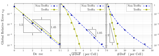
Figure 2: Convergence of the $p$-version. Comparison of the global relative $L^{2}(Q)$ error (51) for Trefftz and non-Trefftz basis functions for the propagation of a smooth wave packet in (1+1)-dimensional space against the polynomial degree (left), the square root of the number of degrees of freedom per element (middle), and the number of degrees of freedom per element (right), respectively.

Figure 3 shows convergence of the $h$-version for degree zero through three. Solid lines correspond to results obtained with the Trefftz basis whereas the dashed lines were obtained using the non-Trefftz basis. Uniform mesh step sizes are applied by reducing $h_{x}$ and $h_{t}$ simultaneously. The Trefftz method exhibits optimal algebraic convergence rates $h^{p+1}$. However, in the non-Trefftz case, the results seem to suggest an odd-even pattern of the convergence rates, with convergence being suboptimal for odd degrees (by one order). Numerical odd-even effects in the convergence rates of DG methods have also been reported, e.g. in [18, section 6.5], although it has been shown in [17] that in some situations this might be a mesh effect, the convergence being always suboptimal on particular meshes.

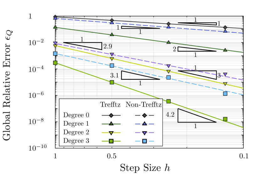
Figure 3: Convergence of the $h$-version. Comparison of the global relative $L^{2}(Q)$ error (51) for Trefftz and non-Trefftz basis functions for the propagation of a smooth wave packet in (1+1)-dimensional space vs. the mesh step size. The spatial and temporal step size $h_{x}$ and $h_{t}$ are decreased simultaneously. Optimal convergence is obtained with the Trefftz basis. In the non-Trefftz case, suboptimal orders of convergence are observed for odd polynomial degrees.

7.4 Stability

As the space–time Trefftz-DG method is implicit in time, a linear system of equations has to be solved for advancing the solution in every time step. In this regard, we investigated the conditioning of the Trefftz and non-Trefftz system matrices. Figure 4 shows that the increase of the conditioning with the polynomial degree in the Trefftz case is very mild, compared to the non-Trefftz case.

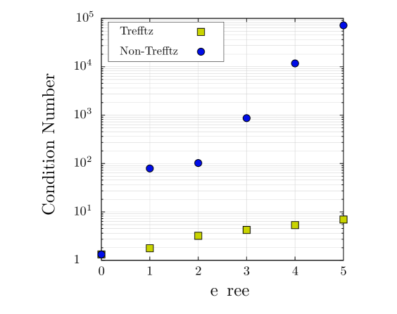
Figure 4: Comparison of the condition number of the update matrix in the Trefftz and non-Trefftz case in dependence of the polynomial degree.

The update matrix is obtained from (50) as $\mathbf{U}=\mathbf{A}^{-1}\,\mathbf{R}$. Note that this matrix is usually not explicitly assembled but we solve for the system (50). In Figure 5 we show eigenvalues of the update matrices with Trefftz basis for degrees $p=0,\ldots,5$. As expected from the stability analysis of section 4.3, all eigenvalues are on or within the unit circle. Figure 5 numerically confirms stability, and it shows the method to be dissipative.

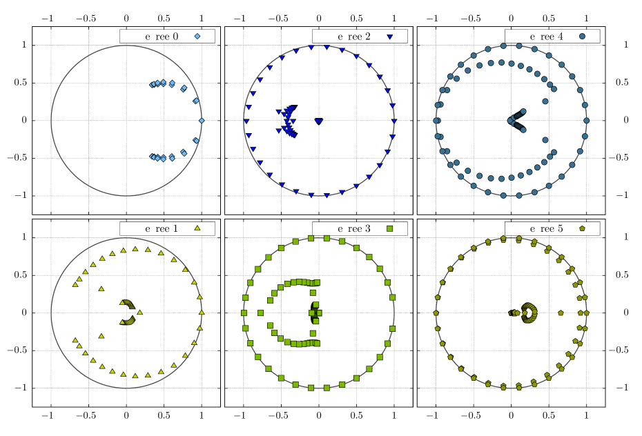
Figure 5: Eigenvalues of update matrices with Trefftz basis and flux stabilisation parameters $\alpha=\beta=0.5$. The grey solid line is the unit circle in the complex plane.

7.5 Flux stabilisation parameters

Let us shortly comment on the choice of the flux stabilisation parameters $\alpha,\beta$. The choice $\alpha=\beta=1/2$ corresponds to a full upwind flux [28] and $\alpha=\beta=0$ (see [25] and also [26]) corresponds to a centred flux. In order to determine the influence onto the numerical error, we varied $\alpha,\beta$ in steps of 0.1 in the range $[0,1]$ and repeated the above example maintaining the same regular mesh with $h_{x}=h_{t}=1$ and polynomial degree $p=2$. Figure 6 depicts the respective global relative error $\epsilon_{Q}$. The minimum error was obtained for $\alpha=1/2$ and $\beta=0$. However, the overall variation of the error is within a factor of two. Similar results are obtained for different settings of the mesh step size and the polynomial degree.

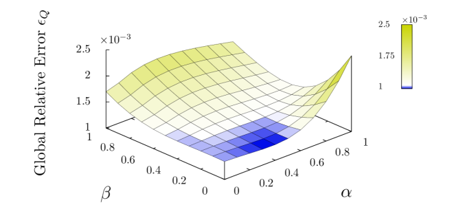
Figure 6: Comparison of the global relative $L^{2}(Q)$ error (51) for the setup described in section 7.2, under variation of the stabilisation parameters $\alpha$ and $\beta$ for a Trefftz basis of degree two (see section 7.5).

8 Conclusions and extensions

In this paper we have analysed a space–time Trefftz discontinuous Galerkin method for linear wave propagation problems. The scheme corresponds to that proposed in [25], with the addition of jump penalisation terms. In one space dimension we proved that the formulation is well-posed and dissipative, and, for polynomial Trefftz trial spaces, we derived a priori $hp$-convergence bounds for its error in DG and $L^{2}$ norm. Numerical examples show the viability of the scheme and confirm the orders of converge.

Several extensions of the analysis developed here can be envisaged. In higher space dimensions, the well-posedness and the abstract error analysis in DG norm are straightforward. In order to prove orders of convergence for the scheme in higher dimensions, new best approximation bounds for Trefftz spaces must be developed, as those derived in section 5 rely on the exact representation of the PDE solution in terms of left- and right-propagating waves, which is a one-dimensional result.

Other topics deserving further investigation are the generalisation of the analysis to unstructured meshes (see [28, 5]) and the derivation of approximation estimates for non-polynomial Trefftz bases. In addition, it would be interesting to analyse the non-penalised case with $\alpha=\beta=0$, as well as other possible less dissipative (or non dissipative) variants.

Appendix A Stability bound in the case of constant coefficients

In the special case of constant material parameters ${\varepsilon}$ and $\mu$, the stability bound (19) can be derived differently from Lemma 4.9, namely using an exact representation of the solution of (18). This results in a simpler constant $C_{\mathrm{stab}}$ with linear, as opposed to exponential, dependence on the total time $T$; no additional assumptions on the flux parameters $\alpha$ and $\beta$ are required.

Lemma A.1.

Assume that ${\varepsilon}$ and $\mu$ are constant in $\Omega$ (and thus in $Q$). The solution $(v_{E},v_{H})$ of the initial auxiliary problem (18) satisfies the stability bound (19) with

$$C_{\mathrm{stab}}^{2}\leq 4Tc\big{(}cN_{\mathrm{hor}}+\eta\gamma N_{\mathrm{ver}}\big{)},$$ (52)

where

$$N_{\mathrm{hor}}:= \;\#\big{\{}t,\text{ such that }(x,t)\in{{\mathcal{F}}_{h}^{\text{hor}}}\cup{{\mathcal{F}}_{h}^{T}}\text{ for some }x_{L}<x<x_{R}\big{\}},$$

$$N_{\mathrm{ver}}:= \;\#\big{\{}x,\text{ such that }(x,t)\in{{\mathcal{F}}_{h}^{\text{ver}}}\cup{{\mathcal{F}}_{h}^{L}}\cup{{\mathcal{F}}_{h}^{R}}\text{ for some }0<t<T\big{\}},$$

$$\eta:= \lceil cT/(x_{R}-x_{L})\rceil,$$

$$\gamma:= \max\Big{\{}\left\|(\beta{\varepsilon})^{-1}+(\alpha\mu)^{-1}\right\|_{L^{\infty}({{\mathcal{F}}_{h}^{\text{ver}}})};\,\left\|(\alpha\mu)^{-1}\right\|_{L^{\infty}({{\mathcal{F}}_{h}^{L}}\cup{{\mathcal{F}}_{h}^{R}})}\Big{\}}.$$

Proof.

We assume that $\phi$ and $\psi$ are continuous in $Q$; the general case will follow by a density argument.

First, we extend the initial problem to the entire space $\mathbb{R}$. Define ${{\widetilde{v}}_{E}},{{\widetilde{v}}_{H}},{\widetilde{\phi}},{\widetilde{\psi}}$ in $\mathbb{R}\times\mathbb{R}^{+}$ as the $2(x_{R}-x_{L})$-periodic functions in $x$ that satisfy ${{\widetilde{v}}_{E}}|_{Q}=v_{E},{{\widetilde{v}}_{H}}|_{Q}=v_{H},{\widetilde{\phi}}|_{Q}=\phi,{\widetilde{\psi}}|_{Q}=\psi$ and such that ${{\widetilde{v}}_{E}}$ and ${\widetilde{\psi}}$ are odd around $x_{L}$ (and consequently also around $x_{R}$), and ${{\widetilde{v}}_{H}}$ and ${\widetilde{\phi}}$ are even around the same points, i.e.

$${{\widetilde{v}}_{E}}(x_{L}+x,t) =-{{\widetilde{v}}_{E}}(x_{L}-x,t),\qquad{{\widetilde{v}}_{H}}(x_{L}+x,t)={{\widetilde{v}}_{H}}(x_{L}-x,t),$$

$${\widetilde{\phi}}(x_{L}+x,t) ={\widetilde{\phi}}(x_{L}-x,t),\qquad{\widetilde{\psi}}(x_{L}+x,t)=-{\widetilde{\psi}}(x_{L}-x,t),\qquad\forall(x,t)\in\mathbb{R}\times\mathbb{R}^{+}.$$

(Note that the absolute values are $(x_{R}-x_{L})$-periodic in $x$.) Since time derivatives preserve parities and space derivatives swap them, the extended functions ${{\widetilde{v}}_{E}}$ and ${{\widetilde{v}}_{H}}$ are continuous and satisfy the extended initial problem

$$\frac{\partial{{\widetilde{v}}_{E}}}{\partial x}+\frac{\partial(\mu{{\widetilde{v}}_{H}})}{\partial t}={\widetilde{\phi}} \;\text{in}\;\mathbb{R}\times\mathbb{R}^{+},$$

$$\frac{\partial{{\widetilde{v}}_{H}}}{\partial x}+\frac{\partial({\varepsilon}{{\widetilde{v}}_{E}})}{\partial t}={\widetilde{\psi}} \;\text{in}\;\mathbb{R}\times\mathbb{R}^{+},$$

$${{\widetilde{v}}_{E}}(\cdot,0)=0,\quad{{\widetilde{v}}_{H}}(\cdot,0)=0 \;\text{on}\;\mathbb{R}.$$

Second, we split the right- and the left-propagating components. Define

$$u:={\varepsilon}^{1/2}{{\widetilde{v}}_{E}}+\mu^{1/2}{{\widetilde{v}}_{H}},\quad w:={\varepsilon}^{1/2}{{\widetilde{v}}_{E}}-\mu^{1/2}{{\widetilde{v}}_{H}},\qquad\text{so that}\qquad{{\widetilde{v}}_{E}}=\frac{u+w}{2{\varepsilon}^{1/2}},\quad{{\widetilde{v}}_{H}}=\frac{u-w}{2\mu^{1/2}}.$$

They satisfy the inhomogeneous transport equations in $\mathbb{R}\times\mathbb{R}^{+}$

$$\frac{\partial u}{\partial x}+\frac{\partial(c^{-1}u)}{\partial t}={\varepsilon}^{1/2}{\widetilde{\phi}}+\mu^{1/2}{\widetilde{\psi}}=:f,\qquad\frac{\partial w}{\partial x}-\frac{\partial(c^{-1}w)}{\partial t}={\varepsilon}^{1/2}{\widetilde{\phi}}-\mu^{1/2}{\widetilde{\psi}}=:g,$$

recalling that $({\varepsilon}\mu)^{1/2}=c^{-1}$, so they can be written explicitly with the following representation formula (e.g. [9, section 2.1.2, equation (5)], recall that from the assumptions made in the proof, $f$ and $g$ are piecewise continuous)

$$u(x,t)=\int_{0}^{t}cf\big{(}x+c(s-t),s\big{)}\,\mathrm{d}s,\qquad w(x,t)=-\int_{0}^{t}cg\big{(}x-c(s-t),s\big{)}\,\mathrm{d}s.$$

We first bound the $L^{2}$ norm of $u$ and $w$ on horizontal and vertical segments with the data $f,g$; from the triangle inequality $({{\widetilde{v}}_{E}},{{\widetilde{v}}_{H}})$ will be bounded by ${\widetilde{\phi}}$ and ${\widetilde{\psi}}$, and the bound for $v_{E}$ and $v_{H}$ will follow. For all $0\leq t\leq T$

$$\left\|u(\cdot,t)\right\|^{2}_{L^{2}(\Omega)} =\int_{x_{L}}^{x_{R}}\Big{(}\int_{0}^{t}cf\big{(}x+c(s-t),s\big{)}\,\mathrm{d}s\Big{)}^{2}\,\mathrm{d}x$$

$$\leq tc^{2}\int_{x_{L}}^{x_{R}}\int_{0}^{t}\big{|}f\big{(}x+c(s-t),s\big{)}\big{|}^{2}\,\mathrm{d}s\,\mathrm{d}x$$

$$=tc^{2}\int_{0}^{t}\int_{x_{L}+c(s-t)}^{x_{R}+c(s-t)}\big{|}f(y,s)\big{|}^{2}\,\mathrm{d}y\,\mathrm{d}s$$

$$\leq 2tc^{2}\int_{0}^{t}\int_{x_{L}+c(s-t)}^{x_{R}+c(s-t)}\big{(}{\varepsilon}|{\widetilde{\phi}}(y,s)|^{2}+\mu|{\widetilde{\psi}}(y,s)|^{2}\big{)}\,\mathrm{d}y\,\mathrm{d}s$$

$$=2tc^{2}\bigg{(}\left\|{\varepsilon}^{1/2}\phi\right\|^{2}_{L^{2}(\Omega\times(0,t))}+\left\|\mu^{1/2}\psi\right\|^{2}_{L^{2}(\Omega\times(0,t))}\bigg{)}$$

(the last equality follows from the symmetries of ${\widetilde{\phi}}$ and ${\widetilde{\psi}}$ which ensure the equality of their $L^{2}$ norms on the rectangle $(x_{L},x_{R})\times(0,t)$ and on the parallelogram with vertices $(x_{L}-ct,0),(x_{R}-ct,0),(x_{R},t),(x_{L},t)$). Similarly, for all $x\in\Omega$

$$\left\|u(x,\cdot)\right\|^{2}_{L^{2}(0,T)} =\int_{0}^{T}\Big{(}\int_{0}^{t}cf\big{(}x+c(s-t),s\big{)}\,\mathrm{d}s\Big{)}^{2}\,\mathrm{d}t$$

$$\leq c^{2}\int_{0}^{T}t\int_{0}^{t}\big{|}f\big{(}x+c(s-t),s\big{)}\big{|}^{2}\,\mathrm{d}s\,\mathrm{d}t$$

$$=c^{2}\int_{0}^{T}\int_{s}^{T}t\big{|}f\big{(}x+c(s-t),s\big{)}\big{|}^{2}\,\mathrm{d}t\,\mathrm{d}s$$

$$=c^{2}\int_{0}^{T}\int_{x-c(T-s)}^{x}\Big{(}\frac{x-y}{c}+s\Big{)}\big{|}f(y,s)\big{|}^{2}\frac{1}{c}\,\mathrm{d}y\,\mathrm{d}s$$

$$\leq 2Tc\int_{0}^{T}\int_{x-c(T-s)}^{x}\big{(}{\varepsilon}|{\widetilde{\phi}}(y,s)|^{2}+\mu|{\widetilde{\psi}}(y,s)|^{2}\big{)}\,\mathrm{d}y\,\mathrm{d}s$$

$$\leq 2Tc\bigg{(}\left\|{\varepsilon}^{1/2}{\widetilde{\phi}}\right\|^{2}_{L^{2}((x-cT,x)\times(0,T))}+\left\|\mu^{1/2}{\widetilde{\psi}}\right\|^{2}_{L^{2}((x-cT,x)\times(0,T))}\bigg{)}$$

$$\leq 2Tc\bigg{\lceil}\frac{cT}{x_{R}-x_{L}}\bigg{\rceil}\bigg{(}\left\|{\varepsilon}^{1/2}\phi\right\|^{2}_{L^{2}(Q)}+\left\|\mu^{1/2}\psi\right\|^{2}_{L^{2}(Q)}\bigg{)},$$

where $\lceil cT/(x_{R}-x_{L})\rceil$ is the number of times $Q$ must be replicated in the $x$ direction to cover the left domain of dependence of $\{x\}\times(0,T)$.

Analogous bounds can be proved for the left-propagating term $w$.

Going back to the solution of the auxiliary problem, we obtain (using ${\varepsilon}v_{E}^{2}\leq(u^{2}+w^{2})/2$, $\mu v_{H}^{2}\leq(u^{2}+w^{2})/2$ and summing over all vertical and horizontal segments)

$$\left\|{\varepsilon}^{1/2}v_{E}\right\|^{2}_{L^{2}({{\mathcal{F}}_{h}^{\text{hor}}}\cup{{{{\mathcal{F}}_{h}^{T}}}})}+\left\|\mu^{1/2}v_{H}\right\|^{2}_{L^{2}({{\mathcal{F}}_{h}^{\text{hor}}}\cup{{{{\mathcal{F}}_{h}^{T}}}})}$$

$$\hskip 28.45274pt+\left\|{\beta^{-1/2}}v_{E}\right\|^{2}_{L^{2}({{\mathcal{F}}_{h}^{\text{ver}}})}+\left\|{\alpha^{-1/2}}v_{H}\right\|^{2}_{L^{2}({{\mathcal{F}}_{h}^{\text{ver}}}\cup{{\mathcal{F}}_{h}^{L}}\cup{{\mathcal{F}}_{h}^{R}})}$$

$$\leq\left\|u\right\|^{2}_{L^{2}({{\mathcal{F}}_{h}^{\text{hor}}}\cup{{\mathcal{F}}_{h}^{T}})}+\left\|w\right\|^{2}_{L^{2}({{\mathcal{F}}_{h}^{\text{hor}}}\cup{{\mathcal{F}}_{h}^{T}})}+\left\|\gamma^{1/2}u\right\|^{2}_{L^{2}({{\mathcal{F}}_{h}^{\text{ver}}}\cup{{\mathcal{F}}_{h}^{L}}\cup{{\mathcal{F}}_{h}^{R}})}+\left\|\gamma^{1/2}w\right\|^{2}_{L^{2}({{\mathcal{F}}_{h}^{\text{ver}}}\cup{{\mathcal{F}}_{h}^{L}}\cup{{\mathcal{F}}_{h}^{R}})}$$

$$\leq 4Tc\big{(}cN_{\mathrm{hor}}+\lceil cT/(x_{R}-x_{L})\rceil\gamma N_{\mathrm{ver}}\big{)}\bigg{(}\left\|{\varepsilon}^{1/2}\phi\right\|^{2}_{L^{2}(Q)}+\left\|\mu^{1/2}\psi\right\|^{2}_{L^{2}(Q)}\bigg{)}.$$

∎

References

• [1] N. Batir, Inequalities for the gamma function, Arch. Math. (Basel), 91 (2008), pp. 554–563.
• [2] A. Buffa and P. Monk, Error estimates for the ultra weak variational formulation of the Helmholtz equation, M2AN, Math. Model. Numer. Anal., 42 (2008), pp. 925–940.
• [3] A. Cangiani, E. H. Georgoulis, and P. Houston, $hp$-version discontinuous Galerkin methods on polygonal and polyhedral meshes, Math. Models Methods Appl. Sci., 24 (2014), pp. 2009–2041.
• [4] O. Cessenat and B. Després, Application of an ultra weak variational formulation of elliptic PDEs to the two-dimensional Helmholtz equation, SIAM J. Numer. Anal., 35 (1998), pp. 255–299.
• [5] F. Costanzo and H. Huang, Proof of unconditional stability for a single-field discontinuous Galerkin finite element formulation for linear elasto-dynamics, Comput. Methods Appl. Mech. Engrg., 194 (2005), pp. 2059–2076.
• [6] E. Deckers, O. Atak, L. Coox, R. D’Amico, H. Devriendt, S. Jonckheere, K. Koo, B. Pluymers, D. Vandepitte, and W. Desmet, The wave based method: An overview of 15 years of research, Wave Motion, 51 (2014), pp. 550–565. Innovations in Wave Modelling.
• [7] R. A. DeVore and G. G. Lorentz, Constructive approximation, vol. 303 of Grundlehren der Mathematischen Wissenschaften [Fundamental Principles of Mathematical Sciences], Springer-Verlag, Berlin, 1993.
• [8] H. Egger, F. Kretzschmar, S. M. Schnepp, I. Tsukerman, and T. Weiland, Transparent boundary conditions in a Discontinuous Galerkin Trefftz method, arXiv preprint arXiv:1410.1899, (2014).
• [9] L. C. Evans, Partial Differential Equations, Graduate Studies in Mathematics, American Mathematical Society, Providence, 3rd ed., 2002.
• [10] R. S. Falk and G. R. Richter, Explicit finite element methods for symmetric hyperbolic equations, SIAM J. Numer. Anal., 36 (1999), pp. 935–952.
• [11] C. Farhat, I. Harari, and U. Hetmaniuk, A discontinuous Galerkin method with Lagrange multipliers for the solution of Helmholtz problems in the mid-frequency regime, Comput. Methods Appl. Mech. Eng., 192 (2003), pp. 1389–1419.
• [12] D. French and T. Peterson, A continuous space-time finite element method for the wave equation, Math. Comp., 65 (1996), pp. 491–506.
• [13] D. A. French, A space-time finite element method for the wave equation, Comput. Methods Appl. Mech. Engrg., 107 (1993), pp. 145–157.
• [14] G. Gabard, Discontinuous Galerkin methods with plane waves for time-harmonic problems, J. Comput. Phys., 225 (2007), pp. 1961–1984.
• [15] C. J. Gittelson, R. Hiptmair, and I. Perugia, Plane wave discontinuous Galerkin methods: analysis of the $h$–version, M2AN Math. Model. Numer. Anal., 43 (2009), pp. 297–332.
• [16] R. Griesmaier and P. Monk, Discretization of the wave equation using continuous elements in time and a hybridizable discontinuous Galerkin method in space, J. Sci. Comput., 58 (2014), pp. 472–498.
• [17] J. Guzmán and B. Rivière, Sub-optimal convergence of non-symmetric discontinuous Galerkin methods for odd polynomial approximations, J. Sci. Comput., 40 (2009), pp. 273–280.
• [18] J. S. Hesthaven and T. Warburton, Nodal Discontinuous Galerkin Methods, Springer, 2008.
• [19] R. Hiptmair, A. Moiola, and I. Perugia, Plane wave discontinuous Galerkin methods for the 2D Helmholtz equation: analysis of the $p$-version, SIAM J. Numer. Anal., 49 (2011), pp. 264–284.
• [20]  , Trefftz discontinuous Galerkin methods for acoustic scattering on locally refined meshes, Appl. Num. Math., 79 (2014), pp. 79–91.
• [21] T. J. R. Hughes and G. M. Hulbert, Space-time finite element methods for elastodynamics: formulations and error estimates, Comput. Methods Appl. Mech. Engrg., 66 (1988), pp. 339–363.
• [22] G. M. Hulbert and T. J. R. Hughes, Space-time finite element methods for second-order hyperbolic equations, Comput. Methods Appl. Mech. Engrg., 84 (1990), pp. 327–348.
• [23] T. Huttunen, P. Monk, and J. P. Kaipio, Computational aspects of the ultra-weak variational formulation, J. Comput. Phys., 182 (2002), pp. 27–46.
• [24] C. Johnson, Discontinuous Galerkin finite element methods for second order hyperbolic problems, Comput. Methods Appl. Mech. Engrg., 107 (1993), pp. 117–129.
• [25] F. Kretzschmar, S. M. Schnepp, I. Tsukerman, and T. Weiland, Discontinuous Galerkin methods with Trefftz approximations, J. Comput. Appl. Math., 270 (2014), pp. 211–222.
• [26] M. Lilienthal, S. M. Schnepp, and T. Weiland, Non-dissipative space-time $hp$-discontinuous Galerkin method for the time-dependent Maxwell equations, J. Comput. Phys., 275 (2014), pp. 589–607.
• [27] A. Macia̧g and J. Wauer, Solution of the two-dimensional wave equation by using wave polynomials, J. Engrg. Math., 51 (2005), pp. 339–350.
• [28] P. Monk and G. R. Richter, A discontinuous Galerkin method for linear symmetric hyperbolic systems in inhomogeneous media, J. Sci. Comput., 22/23 (2005), pp. 443–477.
• [29] P. Monk and D. Wang, A least squares method for the Helmholtz equation, Comput. Methods Appl. Mech. Eng., 175 (1999), pp. 121–136.
• [30] S. Petersen, C. Farhat, and R. Tezaur, A space-time discontinuous Galerkin method for the solution of the wave equation in the time domain, Internat. J. Numer. Methods Engrg., 78 (2009), pp. 275–295.
• [31] C. Schwab, $p$- and $hp$-Finite Element Methods. Theory and Applications in Solid and Fluid Mechanics, Numerical Mathematics and Scientific Computation, Clarendon Press, Oxford, 1998.
• [32] R. Tezaur and C. Farhat, Three-dimensional discontinuous Galerkin elements with plane waves and Lagrange multipliers for the solution of mid-frequency Helmholtz problems, Internat. J. Numer. Methods Engrg., 66 (2006), pp. 796–815.
• [33] L. L. Thompson and P. M. Pinsky, A space-time finite element method for structural acoustics in infinite domains part 1: Formulation, stability and convergence, Comput. Methods Appl. Mech. Eng., 132 (1996), pp. 195–227.
• [34] J. Van der Vegt and H. Van der Ven, Space–time discontinuous Galerkin finite element method with dynamic grid motion for inviscid compressible flows: I. General formulation, J. Comput. Phys., 182 (2002), pp. 546–585.
• [35] D. Wang, R. Tezaur, and C. Farhat, A hybrid discontinuous in space and time Galerkin method for wave propagation problems, Internat. J. Numer. Methods Engrg., 99 (2014), pp. 263–289.