Long–Range Atom–Wall Interactions and Mixing Terms: Metastable Hydrogen

Abstract

We investigate the interaction of metastable $2S$ hydrogen atoms with a perfectly conducting wall, including parity-breaking $S$–$P$ mixing terms (with full account of retardation). The neighboring $2P_{1/2}$ and $2P_{3/2}$ levels are found to have a profound effect on the transition from the short-range, nonrelativistic regime, to the retarded form of the Casimir–Polder interaction. The corresponding $P$ state admixtures to the metastable $2S$ state are calculated. We find the long-range asymptotics of the retarded Casimir–Polder potentials and mixing amplitudes, for general excited states, including a fully quantum electrodynamic treatment of the dipole-quadrupole mixing term. The decay width of the metastable $2S$ state is roughly doubled even at a comparatively large distance of $918\,$atom units (Bohr radii) from the perfect conductor. The magnitude of the calculated effects is compared to the unexplained Sokolov effect.

Introduction.—The investigation of atom-wall interactions for atoms in contact with conducting materials has a long history. Starting from the works of Lennard–Jones LJ1932 , Bardeen Ba1940 , Casimir and Polder CaPo1948 , and Lifshitz Li1955 , research on related matters has found continuously growing interest over the last decades WySi1984 ; WySi1985 ; BaDo1987 ; BaDo1990 . In the non-retarded regime (close range), the interaction energy scales as $1/\mathcal{Z}^{3}$ with the atom-wall distance $\mathcal{Z}$, while for atom-wall distances large in comparison to a typical atomic wavelength, the interaction energy scales as $1/\mathcal{Z}^{4}$ (see Chap. 8 of Ref. Mi1994 ). The leading term is given by virtual dipole transitions, while multipole corrections have recently been analyzed in Ref. LaDKJe2010pra . The symmetry breaking induced by the wall leads to dipole-quadrupole mixing terms, which lead to admixtures to metastable levels BoEtAl2001 ; KaEtAl2006epl . While this effect has been analyzed in the non-retarded van-der-Waals regime BoEtAl2001 ; KaEtAl2006epl , a fully quantum electrodynamic calculation of this effect would be of obvious interest.

This fact is emphasized by the curious observation of a long-range, and conceivably super-long-range (micrometer-scale) interaction of metastable hydrogen $2S$ atoms with a conducting surface (the so-called Sokolov effect, see Refs. SoYaPa1994 ; KaKaKuPoSo1996 ; SoYaPaPc2002 ; SoEtAl2005 ). It is not far-fetched to suspect that this effect could be due to a quantum electrodynamically induced tail of the dipole-quadrupole mixing term in the atom-wall interaction. Namely, for the hydrogen $2S$ atom, the neighboring $2P_{1/2}$ and $2P_{3/2}$ levels are removed only by the Lamb shift and fine-structure, respectively, while it is known that virtual states of lower energy can induce long-range tails in atom-wall interactions, as well as in the Lamb shift between plates (see Refs. Ba1970 ; BaBa1972a ; BaBa1972b ; Ba1974 ; Ba1979 ; Fo1979 ; Ba1987a ; Ba1987b ; Ba1988 ; Ba1997 ). The large admixtures typically induced in atomic systems when a metastable level couples to nearly degenerate states of opposite parity suggest that a closer investigation of the hydrogen system is warranted. Atomic units with $\hbar=4\pi\epsilon_{0}=1$ and $c=1/\alpha$ are used throughout this Rapid Communication, where $\alpha$ is the fine-structure constant. The electron charge is explicitly denoted as $e$ unless stated otherwise.

Retardation of the atom-wall interaction.—The quantum electrodynamic (QED) length-gauge interaction

$$H_{I}=-e\,\vec{r}\cdot\vec{E}-\frac{e}{2}r^{i}\,r^{j}\,\partial E^{i}/\partial r^{j}+\dots\,,$$ (1)

follows naturally from the formalism of long-wavelength QED interaction Hamiltonian PoZi1959 ; Pa2004 ($\vec{r}$ denotes the electron coordinate). In contrast to the vector potential, the electric field strength (operator) is gauge-invariant (this point has given rise to some discussion, see Ref. Ko1978prl ) and reads as [cf. Eq. (2.3) of Ref. Ba1974 ]

$$\vec{E}(\vec{r})= \;\int\limits_{0}^{\infty}\mathrm{d}L\int\limits_{\mathbbm{R}^{2}}\frac{\mathrm{d}^{2}k_{\parallel}}{\pi}\sqrt{\omega}\left\{a_{1}(\vec{k},L)(\hat{k}_{\parallel}\times{\hat{e}}_{z})\sin(Lz)\right.$$

$$\;\left.+a_{2}(\vec{k},L)\,\left[{\hat{k}}_{\parallel}\,\frac{\mathrm{i}L}{\omega}\sin(Lz)-{\hat{e}}_{z}\,\frac{k_{\parallel}}{\omega}\cos(Lz)\right]\right\}$$

$$\;\times\mathrm{e}^{\mathrm{i}\vec{k}_{\parallel}\cdot\vec{r}_{\parallel}}+{\rm h.c.}\,,$$ (2)

where $\vec{r}=\vec{r}_{\parallel}+z\,\hat{e}_{z}$ with $\vec{r}_{\parallel}=x\,\hat{e}_{x}+y\,\hat{e}_{y}$, while $\vec{k}_{\parallel}=k_{x}\,\hat{e}_{x}+k_{y}\,\hat{e}_{y}$, also $\vec{k}_{\perp}=k_{z}\,\hat{e}_{z}$, and $L\equiv|\vec{k}_{\perp}|$. The commutator relation is $[a_{s}(\vec{k}_{\parallel},L),\,a^{\dagger}_{s^{\prime}}(\vec{k}_{\parallel},L)]=\delta_{ss^{\prime}}\,\delta^{(2)}(\vec{k}_{\parallel}-\vec{k}^{\prime}_{\parallel})\,\delta(L-L^{\prime})$ for the annihilation and creation operators $a_{s}$ and $a^{\dagger}_{s}$. In order to evaluate the interaction Hamiltonian (1), one shifts $z\to\mathcal{Z}+z$ where $\mathcal{Z}$ is the coordinate of the atom’s center (nucleus). The proton is at $(0,0,\mathcal{Z})$, while the atomic electron coordinates are $(x,y,\mathcal{Z}+z)$. The surface of the perfect conductor is in the $xy$ plane, i.e., in the plane described by the points $(x,y,0)$. The unperturbed Hamiltonian $H_{0}$ is the sum of the free radiation field and the unperturbed atom [see Eq. (2.1) of Ref. Ba1974 and Eq. (3.2) of Ref. JeKe2004aop ]. For a reference ground state $|n\rangle$, second-order perturbation theory leads to a known result given in Eq. (8.41) of Ref. Mi1994 or Eq. (27) of Ref. LaDKJe2010pra , which involves the symmetric sum with imaginary frequency in the argument of the dynamics polarizability $\Pi(\pm\mathrm{i}\omega)$. The Wick rotation of the virtual photon integration contour, leads to the symmetrization $\mathrm{i}\omega\leftrightarrow-\mathrm{i}\omega$ but cannot be done for excited reference states. We use second-order perturbation theory to evaluate $\Delta E=\langle n|(-e\,\vec{r}\cdot\vec{E})\,[1/(E_{n}-H_{0}^{\prime})]\,(-e\,\vec{r}\cdot\vec{E})|n\rangle$ and obtain [cf. the discussion following Eq. (2.12) of Ref. Ba1974 ],

$$\Delta E\doteq\frac{e^{2}}{2\pi}\,{\mbox{(P.V.)}}\,\sum_{q}\int\limits_{0}^{\infty}\mathrm{d}L\,\int\limits_{L}^{\infty}\mathrm{d}\omega\,\cos(2L\,\mathcal{Z})\,\frac{L^{2}\,\left(\left|\langle n|{\vec{r}}_{\parallel}|q\rangle\right|^{2}+2\,\left|\langle n|z|q\rangle\right|^{2}\right)+\omega^{2}\left(\left|\langle n|{\vec{r}}_{\parallel}|q\rangle\right|^{2}-2\,\left|\langle n|z|q\rangle\right|^{2}\right)}{\mathcal{E}_{q}+\omega-\mathrm{i}\,\delta}\,,$$ (3)

where the identity $\int_{\mathbbm{R}^{3}}\mathrm{d}^{3}k=2\int_{0}^{2\pi}\mathrm{d}\varphi\int_{0}^{\infty}\mathrm{d}L\int_{0}^{\infty}\mathrm{d}\omega\,\omega$  , with $\omega=\sqrt{\vec{k}_{\parallel}^{2}+k_{z}^{2}}$, and $L=|k_{z}|$ has been used in order to transform the integration measure. The virtual states are denoted as $|q\rangle$, and their energy difference to the reference state is denoted as $\mathcal{E}_{q}\equiv E_{q}-E_{n}$. In contrast to the velocity gauge Ba1974 , there is no seagull term to consider, and it is not necessary to add the electrostatic interaction with the mirror charges by hand Le1981qed . It is an in principle well known (see the remarks following Eq. (A.22) in Appendix A of Ref. Sa1967Adv ), but sometimes forgotten wisdom that the Coulomb interaction does not need to be quantized in the velocity gauge Le1981qed . The integration with respect to $\omega$ leads to logarithmic terms [see the Appendix of Ref. Ba1974 ]. After the subtraction of $\mathcal{Z}$-independent terms (the subtraction is denoted by the $\doteq$ sign), one obtains

$$I_{1}(\chi)\doteq \;\int_{0}^{\infty}\mathrm{d}L\,\cos(2L\mathcal{Z})\,\ln(|\mathcal{E}_{q}+L|)=\mathcal{E}_{q}\,\left(\frac{\pi\,[1-\varepsilon(\mathcal{E}_{q})]}{2\chi}-\frac{T(\chi)}{\chi}-\pi\Theta(-\mathcal{E}_{q})\,\frac{2\sin^{2}(\tfrac{\chi}{2})}{\chi}\right)\,,$$ (4a)

$$I_{2}(\chi)\doteq \;-\frac{\partial^{2}I_{1}}{\partial\chi^{2}}=\mathcal{E}_{q}\,\left(\frac{\pi\,[\varepsilon(\mathcal{E}_{q})-1]+\chi}{\chi^{3}}+\frac{2-\chi^{2}}{\chi^{3}}\,T(\chi)-\frac{2}{\chi^{2}}\,U(\chi)+\pi\Theta(-\mathcal{E}_{q})\,\frac{\partial^{2}}{\partial\chi^{2}}\frac{2\sin^{2}(\tfrac{\chi}{2})}{\chi}\right)\,,$$ (4b)

$$T(\chi)= \;\sin(\chi)\,{\mathrm{Ci}}(\chi)-\cos(\chi)\,{\mathrm{Si}}(\chi)+\frac{\pi}{2}\cos(\chi)\,,\qquad\chi=2|\mathcal{E}_{q}|\,\mathcal{Z}\,,\qquad\varepsilon(\mathcal{E}_{q})=\Theta(\mathcal{E}_{q})-\Theta(-\mathcal{E}_{q})\,.$$ (4c)

Here, ${\mathrm{Ci}}(\chi)=-\int_{\chi}^{\infty}\mathrm{d}t\,\frac{\cos(t)}{t}$ and ${\mathrm{Si}}(\chi)=\int_{0}^{\chi}\mathrm{d}t\,\frac{\sin(t)}{t}$, and $U(\chi)=\frac{\partial}{\partial\chi}T(\chi)$, while $T(\chi)=\chi^{-1}-\frac{\partial}{\partial\chi}U(\chi)$. We confirm the result given in Eq. (2.18) of Ref. Ba1974 and represent the “distance-dependent Lamb shift” as

$$\Delta E\doteq \frac{e^{2}}{2\pi}\sum_{q}\mathcal{E}_{q}^{3}\,\biggl{\{}\left(\left|\langle n|{\vec{r}}_{\parallel}|q\rangle\right|^{2}-2\,\left|\langle n|z|q\rangle\right|^{2}\right)\,\left[\frac{\pi\,[\varepsilon(\mathcal{E}_{q})-1]}{2\chi}-\frac{1}{\chi^{2}}+\frac{T(\chi)}{\chi}+\pi\Theta(-\mathcal{E}_{q})\,\frac{1-\cos(\chi)}{\chi}\right]$$ (5)

$$\;-\left(\left|\langle n|{\vec{r}}_{\parallel}|q\rangle\right|^{2}+2\left|\langle n|z|q\rangle\right|^{2}\right)\,\left[\frac{\pi\,[\varepsilon(\mathcal{E}_{q})-1]+\chi}{\chi^{3}}+\frac{2-\chi^{2}}{\chi^{3}}\,T(\chi)-\frac{2}{\chi^{2}}\,U(\chi)+\pi\Theta(-\mathcal{E}_{q})\frac{\partial^{2}}{\partial\chi^{2}}\frac{1-\cos(\chi)}{\chi}\right]\biggr{\}}\,.$$

We should perhaps clarify that the $\mathcal{Z}$-independent contribution to the Lamb shift (the ordinary “free-space Lamb shift”) is absorbed in the subtraction procedure denoted here by the “$\doteq$” sign in Eqs. (4), (5), (7) and (8). The $\mathcal{Z}$-dependent position of the energy level is obtained after adding the “free-space Lamb shift” $\mathcal{L}$ and “free-space fine structure” $\mathcal{F}$ given in Eq. (12) to the $\mathcal{Z}$-dependent energy shifts given in Eqs. (5) and (8). In the nonretardation limit, the $\mathcal{Z}$-dependent results given in Eqs. (5) and (8) are replaced by the respective terms of the nonretarded potential (Long–Range Atom–Wall Interactions and Mixing Terms: Metastable Hydrogen). This (somewhat subtle) point is not fully discussed in previous works on the subject Ba1970 ; BaBa1972a ; BaBa1972b ; Ba1974 ; Ba1979 and therefore should be mentioned for absolute clarity.

The term $-\chi^{-2}$ in the coefficient multiplying $\left|\langle n|{\vec{r}}_{\parallel}|q\rangle\right|^{2}-2\,\left|\langle n|\vec{z}|q\rangle\right|^{2}$ vanishes after summing over the entire spectrum of virtual states; it is obtained naturally in the length gauge and otherwise cancels a term in the expansion of the energy shift for large $\chi$ (even before the application of the sum rule, which is crucial in velocity gauge Ba1974 ). The off-diagonal mixing term leads to to the matrix element $\Delta M=\langle m|(-e\,\vec{r}\cdot\vec{E})\,[1/(E_{n}-H_{0})^{\prime}](-\frac{e}{2}r^{i}\,r^{j}\,(\partial E^{i}/\partial r^{j})|n\rangle+\langle m|{\rm h.c.}|n\rangle$,

$$\Delta M= \;\frac{e^{2}}{4\pi}{\mbox{(P.V.)}}\,\sum_{q}\int\limits_{0}^{\infty}\mathrm{d}L\,\int\limits_{L}^{\infty}\mathrm{d}\omega\,\frac{L\,\sin(2\,L\,\mathcal{Z})}{\mathcal{E}_{q}+\omega-\mathrm{i}\delta}\,\left(L^{2}\,\langle n|\mathcal{T}_{2}|m\rangle-\omega^{2}\,\langle n|\mathcal{T}_{1}|m\rangle\right)\,,$$ (6a)

$$\langle m|\mathcal{T}_{1}|n\rangle= \;\langle m|z|q\rangle\,\langle q|{\vec{r}}^{\,2}_{\parallel}-2\,z^{2}|n\rangle+\langle m|{\rm h.c.}|n\rangle\,,$$ (6b)

$$\langle m|\mathcal{T}_{2}|n\rangle= \;\langle m|z|q\rangle\,\langle q|{\vec{r}}^{\,2}_{\parallel}-2\,z^{2}|n\rangle-2\,\langle m|{\vec{r}}_{\parallel}|q\rangle\cdot\langle q|{\vec{r}}_{\parallel}\,z|n\rangle+\langle m|{\rm h.c.}|n\rangle\,.$$ (6c)

After the subtraction of $\mathcal{Z}$-independent terms, the following two results for $J_{1}(\chi)=\int_{0}^{\infty}\mathrm{d}LL\sin(2L\mathcal{Z})\ln(|\mathcal{E}_{q}+L|)$ and $J_{2}(\chi)=-\partial^{2}J_{1}(\chi)/\partial\chi^{2}$ supplement the analytic integrals given in Eq. (4),

$$J_{1}(\chi)\doteq \;\mathcal{E}_{q}^{2}\left(\varepsilon(\mathcal{E}_{q})\left(\frac{\pi}{2\chi^{2}}-\frac{T(\chi)}{\chi^{2}}+\frac{U(\chi)}{\chi}\right)-\frac{\pi}{2\chi^{2}}+\pi\Theta(-\mathcal{E}_{q})\frac{2\sin^{2}(\tfrac{\chi}{2})-\chi\sin(\chi)}{\chi^{2}}\right),$$ (7a)

$$J_{2}(\chi)\doteq \;\mathcal{E}_{q}^{2}\,\left(\frac{3\,\pi}{\chi^{4}}+\varepsilon(\mathcal{E}_{q})\,\left[\frac{4\chi-3\pi}{\chi^{4}}+\frac{3\,(2-\chi^{2})}{\chi^{4}}T(\chi)+\frac{\chi^{2}-6}{\chi^{3}}\,U(\chi)\right]-\pi\Theta(-\mathcal{E}_{q})\,\frac{\partial^{2}}{\partial\chi^{2}}\frac{2\sin^{2}(\tfrac{\chi}{2})-\chi\sin(\chi)}{\chi^{2}}\right)\,.$$ (7b)

We can finally give the complete result for the mixing term $\Delta M$, with full account of retardation, as a sum over virtual states $|q\rangle$,

$$\Delta M\doteq \frac{e^{2}}{4\pi}\sum_{q}\mathcal{E}_{q}^{4}\,\Biggl{\{}\langle m|\mathcal{T}_{1}|n\rangle\,\left[\varepsilon(\mathcal{E}_{q})\,\left(\frac{4+\pi\chi}{2\,\chi^{3}}-\frac{T(\chi)}{\chi^{2}}+\frac{U(\chi)}{\chi}\right)-\frac{\pi}{2\chi^{2}}+\pi\Theta(-\mathcal{E}_{q})\,\frac{2\sin^{2}(\tfrac{\chi}{2})-\chi\,\sin(\chi)}{\chi^{2}}\right]$$ (8)

$$\;+\langle m|\mathcal{T}_{2}|n\rangle\left[\varepsilon(\mathcal{E}_{q})\left(\frac{3\pi-4\,\chi}{\chi^{4}}+\frac{3(\chi^{2}-2)}{\chi^{4}}T(\chi)+\frac{6-\chi^{2}}{\chi^{3}}U(\chi)\right)-\frac{3\pi}{\chi^{4}}+\pi\Theta(-\mathcal{E}_{q})\frac{\partial^{2}}{\partial\chi^{2}}\frac{2\sin^{2}(\tfrac{\chi}{2})-\chi\sin(\chi)}{\chi^{2}}\right]\Biggr{\}}\,.$$

The energy variable $\mathcal{E}_{q}$ is defined with respect to the reference state; i.e., if one evaluates the $|m\rangle$-state admixture to the reference state $|n\rangle$, then one sets $\mathcal{E}_{q}=E_{q}-E_{n}$. For excited reference states, results for both $\Delta E$ given in Eq. (5) and $\Delta M$ in Eq. (8) contain long-range retardation tails for excited reference states,

$$\Delta E= \;e^{2}\,\sum_{q}\Theta(-\mathcal{E}_{q})\,\left[|\langle n|\vec{r}_{\parallel}|q\rangle|^{2}\,\left(\frac{\mathcal{E}_{q}^{2}\,\cos(2\mathcal{E}_{q}\mathcal{Z})}{2\,\mathcal{Z}}-\frac{\mathcal{E}_{q}\,\sin(2\mathcal{E}_{q}\mathcal{Z})}{4\,\mathcal{Z}^{2}}-\frac{\cos(2\mathcal{E}_{q}\mathcal{Z})}{8\,\mathcal{Z}^{3}}\right)\right.$$

$$\;\left.-\,|\langle n|z|q\rangle|^{2}\,\left(\frac{\mathcal{E}_{q}\,\sin(2\,\mathcal{E}_{q}\,\mathcal{Z})}{\mathcal{Z}^{2}}+\frac{\cos(2\mathcal{E}_{q}\mathcal{Z})}{4\,\mathcal{Z}^{3}}\right)\right]-\frac{1}{8\,\pi\,\mathcal{Z}^{4}}\,\left(2\Pi_{\parallel}+\Pi_{\perp}\right)\,,\qquad\qquad\mathcal{Z}\gg\frac{1}{\mathcal{E}_{q}}\,,$$

$$\Pi_{\parallel}= \;\frac{1}{2}\,\sum_{q,\pm}\frac{2}{\mathcal{E}_{q}}\,\langle n|\vec{r}_{\parallel}|q\rangle\cdot\langle q|\vec{r}_{\parallel}|n\rangle\,,\qquad\Pi_{\perp}=\sum_{q,\pm}\frac{2}{\mathcal{E}_{q}}\,\left|\langle n|z|q\rangle\right|^{2}\,,\quad\Pi(\omega)=\frac{e^{2}}{3}\sum_{\pm}\left<n\left|r^{i}\left(\frac{1}{\mathcal{E}_{q}\pm\omega}\right)r^{i}\right|n\right>\,,$$ (9)

where $\Pi_{\parallel}$ and $\Pi_{\perp}$ are the longitudinal and transverse static polarizabilities [for the ground state, $\Pi_{\perp}=\Pi_{\parallel}=\Pi(0)$]. The mixing term has the following long-range asymptotics,

$$\Delta M= \;e^{2}\sum_{q}\Theta(-\mathcal{E}_{q})\,\langle m|{\vec{r}}_{\parallel}|q\rangle\cdot\langle q|{\vec{r}}_{\parallel}\,z|n\rangle\left(-\frac{\mathcal{E}_{q}^{3}\sin(2\mathcal{E}_{q}\,\mathcal{Z})}{4\mathcal{Z}}-\frac{3\,\mathcal{E}_{q}^{2}\cos(2\mathcal{E}_{q}\,\mathcal{Z})}{8\mathcal{Z}^{2}}+\frac{3\,\mathcal{E}_{q}\,\sin(2\mathcal{E}_{q}\,\mathcal{Z})}{8\mathcal{Z}^{3}}+\frac{3\,\mathcal{E}_{q}^{4}\,\cos(2\mathcal{E}_{q}\,\mathcal{Z})}{16\mathcal{Z}^{4}}\right)$$

$$\;+e^{2}\sum_{q}\Theta(-\mathcal{E}_{q})\,\langle m|z|q\rangle\langle q|\vec{r}_{\parallel}^{\,2}-2z^{2}|n\rangle\left(\frac{\mathcal{E}_{q}^{2}\,\cos(2\mathcal{E}_{q}\,\mathcal{Z})}{8\mathcal{Z}^{2}}-\frac{3\,\mathcal{E}_{q}\,\sin(2\mathcal{E}_{q}\,\mathcal{Z})}{16\mathcal{Z}^{3}}-\frac{3\,\cos(2\mathcal{E}_{q}\,\mathcal{Z})}{32\mathcal{Z}^{4}}\right)$$ (10)

$$\;+\frac{e^{2}}{\pi\,\mathcal{Z}^{5}}\sum_{q}\frac{1}{\mathcal{E}_{q}}\left(-\frac{1}{8}\,\langle m|z|q\rangle\,\langle q|{\vec{r}}_{\parallel}^{\,2}|n\rangle+\frac{1}{4}\,\langle m|z|q\rangle\,\langle q|z^{2}|n\rangle+\frac{3}{8}\,\langle m|{\vec{r}}_{\parallel}|q\rangle\cdot\langle q|{\vec{r}}_{\parallel}\,z|n\rangle\right)+\langle m|{\rm h.c.}|n\rangle\,,\qquad\mathcal{Z}\gg\frac{1}{\mathcal{E}_{q}}\,.$$

The results (5) and (8) will now be applied to metastable hydrogen.

Nonretarded admixtures to metastable hydrogen.—The results given in Eq. (5) and (8) have a rather involved analytic structure. In the short-range limit, these results can be compared to the static interaction of the electron and proton Ch1968 ; ErrorChaplik with their respective mirror charges. This interaction leads to the following nonretarded potential (from now on we set the elementary charge $e=1$),

$$V= \;\frac{1}{2}\,\left(-\frac{1}{2(z+\mathcal{Z})}+\frac{2}{\sqrt{x^{2}+y^{2}+(z+2\mathcal{Z})^{2}}}-\frac{1}{2\mathcal{Z}}\right)$$

$$= \;-\frac{{\vec{r}}_{\parallel}^{2}+2z^{2}}{16\,\mathcal{Z}^{3}}+\frac{3z\,({\vec{r}}_{\parallel}^{2}+2z^{2})}{32\,\mathcal{Z}^{4}}+\cdots$$ (11)

where we ignore terms of order $1/\mathcal{Z}^{5}$ and higher factor ; CTDiLa1978vol2 . After some tedious, but straightforward algebra, one can convince oneself that the terms of order $\mathcal{Z}^{-3}$ and $\mathcal{Z}^{-4}$ are in agreement with the short-range asymptotics of the results given in Eqs. (5) and (8), i.e., in the regime $\mathcal{Z}\ll 1/\mathcal{E}_{q}$, which is equivalent to the limit $\chi\to 0$.

For close approach of the atom to the wall, the interaction energy is well described by the static potential (Long–Range Atom–Wall Interactions and Mixing Terms: Metastable Hydrogen), which necessitates a diagonalization of the Schrödinger Hamiltonian plus the nonretarded potential $V$ (both “diagonal” interaction and Lamb shift or fine structure terms, as well as “mixing” terms) in the basis of the $|2S_{1/2}\rangle$, $|2P_{1/2}\rangle$, and $|2P_{3/2}\rangle$ Schrödinger–Pauli wave functions with magnetic projection $\mu=+1/2$, to form the manifestly coupled states $|\mathcal{S}_{1/2}\rangle$, $|\mathcal{P}_{1/2}\rangle$, and $|\mathcal{P}_{3/2}\rangle$. We denote the (free-space) fine-structure and the Lamb shift interval as

$$\mathcal{F}=1.66\times 10^{-6}\,{\rm a.u.}\,,\qquad\mathcal{L}=1.61\times 10^{-7}\,{\rm a.u.}\,,$$ (12)

respectively. According to the adiabatic theorem BoFo1928 ; Ka1950 ; AvEl1999 , the $|\mathcal{S}_{1/2}\rangle$ state eigenvector has the form

$$|\mathcal{S}_{1/2}\rangle\approx \;a_{S}\,|2S_{1/2}\rangle+a_{\frac{1}{2}}\,|2P_{1/2}\rangle+a_{\frac{3}{2}}\,|2P_{3/2}\rangle\,,$$ (13a)

$$a_{S}= \;1\,,\quad a_{\frac{1}{2}}=\frac{\sqrt{3}}{2}\frac{15}{\mathcal{L}\,\mathcal{Z}^{4}}\,,\quad a_{\frac{3}{2}}=\sqrt{\frac{3}{2}}\frac{15}{\mathcal{F}\,\mathcal{Z}^{4}}\,,$$ (13b)

$$1/\mathcal{L}\gg \;\mathcal{Z}\gg 1/\mathcal{L}^{1/4}\,,\qquad 1/\mathcal{Z}\gg\mathcal{Z}\gg 1/\mathcal{F}^{1/4}\,,$$ (13c)

where we ignore higher-order terms in the expansion in inverse powers of $\mathcal{Z}$. The absolute square of the admixture is given by

$$\Xi=\frac{675}{2}\,\left(\frac{1}{\mathcal{F}^{2}}+\frac{1}{2\,\mathcal{L}^{2}}\right)\frac{1}{\mathcal{Z}^{8}}=\frac{6.63\times 10^{15}}{\mathcal{Z}^{8}}\,{\rm a.u.}\,.$$ (14)

The one-photon decay width of the $2P$ state is given as $\Gamma_{2P}=6.27\times 10^{8}\;\frac{{\rm rad}}{{\rm s}}=1.51\times 10^{-8}\;{\rm a.u.}$, whereas the two-photon decay width of the $2S$ state reads $\Gamma_{2S}=8.229\;\frac{{\rm rad}}{{\rm s}}=1.99\times 10^{-16}\;{\rm a.u.}$. The effective decay rate $\Gamma_{\rm eff}$ at a distance $\mathcal{Z}$ is

$$\Gamma_{\rm eff}=\Gamma_{2S}+\Gamma_{2P}\Xi=\left(1.99\times 10^{-16}+\frac{1.01\times 10^{8}}{\mathcal{Z}^{8}}\right)\!{\rm a.u.}.$$ (15)

We have $\Gamma_{\rm eff}=2\,\Gamma_{2S}$ for $\mathcal{Z}_{0}=918\,{\rm a.u.}$. The leading (nonretarded) term in the atom-wall energy shift at this distance amounts to $-7\mathcal{Z}_{0}^{-3}/2=-4.52\times 10^{-9}\;{\rm a.u.}$ and approximates both the single-particle perturbative shift given in Eq. (5) as well as the adiabatic energy of the coupled $|\mathcal{S}_{1/2}\rangle$ state obtained from the diagonalization of the potential (Long–Range Atom–Wall Interactions and Mixing Terms: Metastable Hydrogen) to within 10 %. The atom-wall energy at $\mathcal{Z}_{0}$ is equal to $-29.7\,{\rm MHz}$ and thus much smaller than the Lamb shift and fine structure.

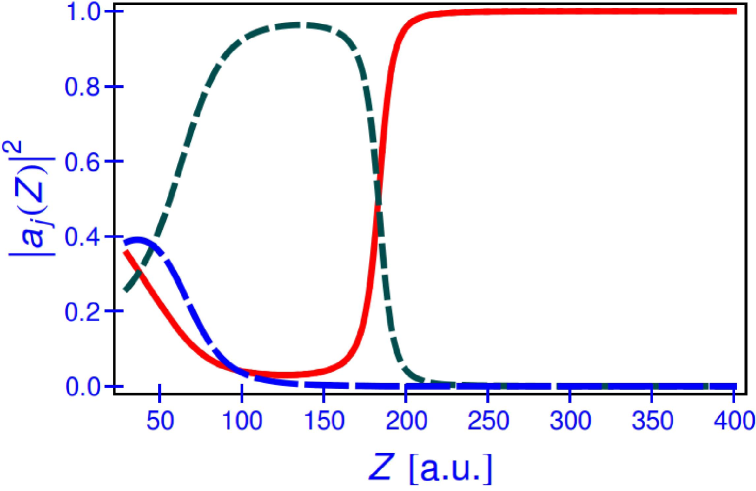
Figure 1: (Color.) The modulus-squared admixtures to the coupled $|\mathcal{S}_{1/2}\rangle$ state are obtained from a diagonalization of the potential (Long–Range Atom–Wall Interactions and Mixing Terms: Metastable Hydrogen) in the basis of $|\mathcal{S}_{1/2}\rangle$, $|\mathcal{P}_{1/2}\rangle$, and $|\mathcal{P}_{3/2}\rangle$ states, for close approach of the atom toward the wall. The subscript $j$ in Eq. (13) takes on the values $j=S$, as well as $j=1/2$ and $j=3/2$ and denotes the state responsible for the admixture. As the $|\mathcal{S}_{1/2}\rangle$ state approaches the wall, the initially dominant $|S_{1/2}\rangle$ state contribution (solid curve, $j=S$) gradually fades and the $|P_{1/2}\rangle$ admixture (short-dashed curve, $j=1/2$) increases, while a significant admixture of the $|P_{3/2}\rangle$ state (long-dashed curve, $j=3/2$), is observed only for close approach. The atom-wall interaction energy becomes commensurate with the Lamb shift and fine structure at $\mathcal{Z}\approx 84$ and at $\mathcal{Z}\approx 184$, respectively.

The admixture formulas for the coupled $|\mathcal{P}_{1/2}\rangle$ state reads as

$$|\mathcal{P}_{1/2}\rangle\approx \;b_{S}\,|2S_{1/2}\rangle+b_{1/2}\,|2P_{1/2}\rangle+b_{3/2}\,|2P_{3/2}\rangle\,,$$ (16a)

$$b_{S}= \;-\sqrt{\frac{3}{4}}\frac{15}{\mathcal{L}\,\mathcal{Z}^{4}}\,,\quad b_{\frac{3}{2}}=\frac{1}{2\,\sqrt{2}}\,\frac{1}{\mathcal{F}\,\mathcal{Z}^{3}}\,,$$ (16b)

and $b_{\frac{1}{2}}=1$. The $|\mathcal{P}_{3/2}\rangle$ state reads as follows,

$$|\mathcal{P}_{3/2}\rangle\approx \;c_{S}\,|2S_{1/2}\rangle+c_{1/2}\,|2P_{1/2}\rangle+c_{3/2}\,|2P_{3/2}\rangle\,,$$ (17a)

$$c_{S}= \;-\sqrt{\frac{3}{2}}\frac{15}{\mathcal{F}\,\mathcal{Z}^{4}},\quad c_{\frac{1}{2}}=\frac{1}{2\sqrt{2}}\frac{1}{(\mathcal{L}+\mathcal{F})\,\mathcal{Z}^{3}},$$ (17b)

and of course $c_{\frac{3}{2}}=1$. For very close approach $Z\lesssim 300$, higher-order terms in the expansion of the potential $V$ [see Eq. (Long–Range Atom–Wall Interactions and Mixing Terms: Metastable Hydrogen)] gradually become important. [These are obtained by straightforward expansion of the potential (Long–Range Atom–Wall Interactions and Mixing Terms: Metastable Hydrogen).] Numerically determined admixtures of the coupled $|\mathcal{S}_{1/2}\rangle$ are given in Fig. 1, they do not follow the asymptotic formulas for very close approach.

Long-range tails.—The oscillatory repulsive-attractive dominant term in the long-range limit of the energy shift, for the $2S$ level, goes as [see Eqs. (5) and (Long–Range Atom–Wall Interactions and Mixing Terms: Metastable Hydrogen)],

$$\Delta E_{2S}\sim\frac{9\mathcal{L}^{2}\,\cos(2\mathcal{L}\,\mathcal{Z})}{2\mathcal{Z}}\,,\qquad\mathcal{Z}\gg\frac{1}{\mathcal{L}}\,,$$ (18)

where we have isolated the leading term from Eq. (Long–Range Atom–Wall Interactions and Mixing Terms: Metastable Hydrogen), setting $\mathcal{E}_{q}=-\mathcal{L}$ and carrying the summation over the virtual levels $|q\rangle=|2P_{1/2}\rangle$ with magnetic projections $\mu=\pm 1/2$. Somewhat surprisingly, the oscillatory terms in Eq. (Long–Range Atom–Wall Interactions and Mixing Terms: Metastable Hydrogen) vanish for virtual $|2P_{1/2}\rangle$ states, so that the long-range coupling to the lower-lying $P$ state vanishes. The leading terms in the long-range asymptotics of the admixture coefficients read as follows [see Eq. (13)],

$$a_{1/2}\sim \;\frac{3\,\sqrt{3}}{\pi\,\mathcal{L}\,\mathcal{F}\,\mathcal{Z}^{5}}\,,\qquad\qquad\mathcal{Z}\gg\frac{1}{\mathcal{L}}\,,$$ (19a)

$$a_{3/2}\sim \;-\sqrt{\frac{3}{2}}\,\frac{3\,\mathcal{L}^{3}}{\mathcal{F}\,\mathcal{Z}}\,\sin(2\mathcal{L}\,\mathcal{Z})\,,\qquad\mathcal{Z}\gg\frac{1}{\mathcal{L}}\,.$$ (19b)

The long-range asymptotic tail of the $P_{3/2}$-state admixture has an oscillatory ($1/\mathcal{Z}$)-form [see Eqs. (Long–Range Atom–Wall Interactions and Mixing Terms: Metastable Hydrogen) and (19b)]. If this tail were not suppressed by the prefactor $\mathcal{L}^{3}/\mathcal{F}$, then it could have easily provided a theoretical explanation for the Sokolov effect SoYaPa1994 ; KaKaKuPoSo1996 ; SoYaPaPc2002 ; SoEtAl2005 , because the $(1/\mathcal{Z})$-interaction has the required functional form to describe a super-long-range term. The tail is created by virtual $|q\rangle=|2P_{1/2}\rangle$ states in Eq. (Long–Range Atom–Wall Interactions and Mixing Terms: Metastable Hydrogen), which are energetically lower than the reference $|2S\rangle$ state. The prefactor of the super-long-range tail of the admixture term depends on details of the spectrum of the atomic system and could be larger for other atoms. For the $P_{1/2}$-state admixture (term $a_{1/2}$), retardation changes the $1/\mathcal{Z}^{4}$ asymptotics for short range to a $1/\mathcal{Z}^{5}$ asymptotics at long range. A full QED treatment of the admixture terms is required for both results recorded in Eqs. (19a) and (19b).

Conclusions.—We can safely conclude that the curious observations reported in SoYaPa1994 ; KaKaKuPoSo1996 ; SoYaPaPc2002 ; SoEtAl2005 regarding super-long-range $2S$–$2P$ mixing terms near metal surfaces cannot find an explanation in terms of a long-range effect involving quantum fluctuations. Both the energy shift (Long–Range Atom–Wall Interactions and Mixing Terms: Metastable Hydrogen) as well as the mixing term (Long–Range Atom–Wall Interactions and Mixing Terms: Metastable Hydrogen) have long-range tails proportional to $1/\mathcal{Z}$, but the energy numerator for the $2S$–$2P_{1/2}$ transition is so small (Lamb shift, a $30\,{\rm cm}$ wavelength transition) that the region in which the $1/\mathcal{Z}$ terms dominate is restricted to excessively large atom-wall separations where the single power of $\mathcal{Z}$ in the denominator is sufficient to make the interaction energy and admixture terms negligible. (We should add that the inclusion of additional mirror charges in a cavity as opposed to a wall can be taken into account, in the short-range limit, by summing the mirror charge interactions into a generalized Riemann zeta function LuRa1985 and therefore cannot change the order-of-magnitude of the admixture terms.)

If the observations reported in Refs. SoYaPa1994 ; KaKaKuPoSo1996 ; SoYaPaPc2002 ; SoEtAl2005 had found a natural explanation in terms of a QED effect, then this might have had significant implications for a typical atomic beam apparatus FiEtAl2004 used in high-precision spectroscopy of atoms, potentially shifting the frequency of transitions involving $2S$ atoms in a narrow tube. For atom-wall separations smaller than $1000$ Bohr radii, substantial admixture terms are found, and the $1/\mathcal{Z}^{8}$ scaling of the effective $2S$ decay rate predicted by Eq. (14) could be tested against an experiment. The clarification of the parity-breaking admixture terms also is important for other precision measurements in atomic physics which involve metastable states, such as EDM and weak-interaction experiments WuMuJe2012prx ; BeGaNa2007paper1 ; BeGaNa2007paper2 ; BuDMCoZo1994 ; NgEtAl1997 ; WeLeBu2013 . The fully retarded expression for the mixing term, given in Eq. (Long–Range Atom–Wall Interactions and Mixing Terms: Metastable Hydrogen), formulates higher-order QED corrections to atom-wall interactions beyond dipole order. Generalization of the formulas to, e.g., the $2^{3}S_{1}$ mestable state of helium is straightforward. One just sums the interactions over the electron coordinates.

References

• (1) J. E. Lennard-Jones, Trans. Faraday Soc. 28, 334 (1932).
• (2) J. Bardeen, Phys. Rev. 58, 727 (1940).
• (3) H. B. G. Casimir and D. Polder, Phys. Rev. 73, 360 (1948).
• (4) E. M. Lifshitz, Zh. Éksp. Teor. Fiz. 29, 94 (1955), [Sov. Phys. JETP 2, 73 (1956)].
• (5) J. M. Wylie and J. E. Sipe, Phys. Rev. A 30, 1185 (1984).
• (6) J. M. Wylie and J. E. Sipe, Phys. Rev. A 32, 2030 (1985).
• (7) A. O. Barut and J. P. Dowling, Phys. Rev. A 36, 2550 (1987).
• (8) A. O. Barut and J. P. Dowling, Phys. Rev. A 41, 2284 (1990).
• (9) P. W. Milonni, The Quantum Vacuum (Academic Press, San Diego, 1994).
• (10) G. Łach, M. DeKieviet, and U. D. Jentschura, Phys. Rev. A 81, 052507 (2010).
• (11) M. Boustimi, B. Viaris de Lesegno, J. Baudon, J. Robert, and M. Ducloy, Phys. Rev. Lett. 86, 2766 (2001).
• (12) J.-C. Karam et al., Europhys. Lett. 74, 36 (2006).
• (13) Y. L. Sokolov, V. P. Yakovlev, and V. G. Pal’chikov, Phys. Scr. T 49, 86 (1994).
• (14) B. B. Kadomtsev, M. B. Kadomtsev, Y. A. Kucheryaev, Y. L. Podogov, and Y. L. Sokolov, Phys. Scr. T 54, 156 (1996).
• (15) Y. L. Sokolov, V. P. Yakovlev, V. G. Pal’chikov, and Y. A. Pchelin, Eur. Phys. J. D 20, 27 (2002).
• (16) Y. L. Sokolov, V. P. Yakovlev, V. G. Pal’chikov, and Y. A. Pchelin, Pis’ma v ZhETF 81, 780 (2005), [JETP Lett. 81, 644 (2005)].
• (17) G. Barton, Proc. Roy. Soc. London, Ser. A 320, 251 (1970).
• (18) M. Babiker and G. Barton, Proc. Roy. Soc. London, Ser. A 326, 255 (1978).
• (19) M. Babiker and G. Barton, Proc. Roy. Soc. London, Ser. A 326, 277 (1972).
• (20) G. Barton, J. Phys. B 7, 2134 (1974).
• (21) G. Barton, Proc. Roy. Soc. London, Ser. A 367, 117 (1979).
• (22) L. H. Ford, Proc. Roy. Soc. London, Ser. A 368, 311 (1979).
• (23) G. Barton, Proc. Roy. Soc. London, Ser. A 410, 141 (1987).
• (24) G. Barton, Proc. Roy. Soc. London, Ser. A 410, 175 (1987).
• (25) G. Barton, Phys. Scr. T 21, 11 (1988).
• (26) G. Barton, Proc. Roy. Soc. London, Ser. A 453, 2461 (1997).
• (27) E. A. Power and S. Zienau, Phil. Trans. R. Soc. Lond. A 251, 427 (1959).
• (28) K. Pachucki, Phys. Rev. A 69, 052502 (2004).
• (29) D. H. Kobe, Phys. Rev. Lett. 40, 538 (1978).
• (30) U. D. Jentschura and C. H. Keitel, Ann. Phys. (N.Y.) 310, 1 (2004).
• (31) T. D. Lee, Particle Physics and Introduction to Field Theory (Harwood Publishers, Newark, NJ, 1981).
• (32) J. J. Sakurai, Advanced Quantum Mechanics (Addison-Wesley, Reading, MA, 1967).
• (33) A. V. Chaplik, Zh. Éksp. Teor. Fiz. 54, 332 (1968), [JETP 27, 178 (1968)].
• (34) The nonretarded potential used in Ref. Ch1968 for the analysis of a related problem, is incomplete as it neglects the interaction of the proton with its mirror charge.
• (35) The well-known prefactor $1/2$ stands because the electric field is zero inside the conductor (see Chap. 11 of Ref. CTDiLa1978vol2 ).
• (36) C. Cohen-Tannoudji, B. Diu, and F. Lalo$\ddot{e}$, Quantum Mechanics (Volume 2), 1 ed. (J. Wiley & Sons, New York, 1978).
• (37) M. Born and V. A. Fock, Z. Phys. A 51, 165 (1928).
• (38) T. Kato, J. Phys. Soc. Jpn. 5, 435 (1950).
• (39) J. E. Avron and A. Elgart, Commun. Math. Phys. 203, 445 (1999).
• (40) C. A. Lütken and F. Ravndal, Phys. Rev. A 31, 2082 (1985).
• (41) M. Fischer et al., Phys. Rev. Lett. 92, 230802 (2004).
• (42) B. J. Wundt, C. T. Munger, and U. D. Jentschura, Phys. Rev. X 2, 041009 (2012).
• (43) T. Bergmann, T. Gasenzer, and O. Nachtmann, Eur. Phys. J. D 45, 197 (2007).
• (44) T. Bergmann, T. Gasenzer, and O. Nachtmann, Eur. Phys. J. D 45, 211 (2007).
• (45) D. Budker, D. DeMille, E. D. Commins, and M. S. Zolotorev, Phys. Rev. A 50, 132 (1994).
• (46) A. T. Nguyen, D. Budker, D. DeMille, and M. Zolotorev, Phys. Rev. A 56, 3453 (1997).
• (47) C. T. M. Weber, N. Leefer, and D. Budker, Phys. Rev. A 88, 062503 (2013).