Three-body recombination of two-component cold atomic gases into deep dimers in an optical model

Abstract

We consider three-body recombination into deep dimers in a mass-imbalanced two-component atomic gas. We use an optical model where a phenomenological imaginary potential is added to the lowest adiabatic hyper-spherical potential. The consequent imaginary part of the energy eigenvalue corresponds to the decay rate or recombination probability of the three-body system. The method is formulated in details and the relevant qualitative features are discussed as functions of scattering lengths and masses. We use zero-range model in analyses of recent recombination data. The dominating scattering length is usually related to the non-equal two-body systems. We account for temperature smearing which tends to wipe out the higher-lying Efimov peaks. The range and the strength of the imaginary potential determine positions and shapes of the Efimov peaks as well as the absolute value of the recombination rate. The Efimov scaling between recombination peaks is calculated and shown to depend on both scattering lengths. Recombination is predicted to be largest for heavy-heavy-light systems. Universal properties of the optical parameters are indicated. We compare to available experiments and find in general very satisfactory agreement.

I Introduction

The Efimov effect is very well established and the energies and radii of the infinitely many three-body bound Efimov states occur in geometric series corresponding to well defined scaling factors depending on the masses of the particles. These states have been searched for and found, but only indirectly as enhanced decay probabilities when the two-body interactions are tuned to specific values. Most of these findings are for three identical atoms where the geometric scaling factor is $22.7$ independent of the atomic mass, see for example the experiments Ottenstein2008 -Huang2014 . The occurrence conditions for the Efimov effect are that at least two of the three two-body subsystems simultaneously interact with infinitely large scattering lengths, or equivalently with bound states of zero energy.

The necessary fine-tuning is most easily achieved when at least two of the particles are identical. Then obviously at least two subsystems are identical and therefore simultaneously fine-tuned in an experiment. If furthermore one of the particles is distinctly different, the scaling factors can differ enormously for the resulting Efimov spectra. When the system has one light and two heavy particles, the scaling factor, or the energy spacing, is very small. This is a huge advantage since many energies then are within the experimentally accessible range. The opposite case of one heavy and two light particles has correspondingly large energy spacing and fewer accessible states.

The two-component gases, where mass-imbalanced three-body systems are likely to recombine in the decay process into a deeply bound dimer and a third particle, are more difficult to prepare in sufficiently cold tunable states. However, several systems are now investigated experimentally pires2014 ; tung2014 ; ulmanis2015 and probably more are in the pipeline.

It is therefore very timely to investigate these processes theoretically zinner2014 in more details and more systematically than done before, where one of the foci has been on the special case of vanishing scattering length between the two similar particles, see for example Hammer2010 . We shall in this paper only consider negative scattering lengths where the final state in the recombination product is a deeply bound dimer, unavailable in usual zero-range three-body models. The theoretical formulation is simplest for three equal masses, since then the single, and necessarily large, scattering length is the only parameter which therefore completely determines the properties of the process. The two-component system is much more complicated, since two scattering lengths and one mass ratio are the necessary parameters to characterize the system.

The scaling factor is very well known as function of masses in the limit of very large scattering lengths Fedorov2003 ; Braaten2006 , that is when both are infinitely large and when only that of the non-equal particles is large while the third between identical particles is vanishingly small. These two extreme limits of different scalings between energies would lead to different periodicities in the enhanced recombination probability as function of the scattering lengths. Any intermediate energy scaling is also possible, and a smooth transition between these limits arises by varying the third scattering length between zero and infinity.

One established method is based on a multiple scattering approach where the final state somehow is simulated although never directly present. Recently a novel suggestion appeared to use an optical model to describe absorption as in nuclear physics and for light waves in materials. This formulation can only provide decay, or absorption, probability without any details of the final states populated in these processes. However, this is all we need to describe the measurable recombination probabilities. In the present report we shall elaborate and explore the properties of this optical model.

The overall purpose of the present paper is to discuss three-body recombination processes in atomic gases. The emphasis is on two-component atomic gases where mass-imbalanced recombination processes are prominent and probably dominating. This shall be done by introducing the details of a simple optical model where the real part is the lowest adiabatic hyper-spherical potential, and the imaginary part is a square well in hyper-radius.

The initial zero-range potential must be regularized to provide physical results. This is achieved by replacing the diverging real part with a constant at small hyper-radii where the imaginary part also is finite. This constant is unimportant for the calculated recombination rates. Such an optical model formulation is phenomenological by nature, but we shall indicate a possible relation to universally determined values of the model parameters.

The paper is structured with basic definitions in section II, while the focus on computation of mass-imbalanced three-body recombinations is formulated in details in section III. The choice and dependence on physical as well as model parameters are discussed in section IV. Precise comparison to available experimental results is the content of section V. Finally, we summarize a number of conclusions in section VI, where we also suggest interesting future research projects.

II Notation and basic ingredients

In this section we sketch the details necessary to calculate the potential which provides the wave functions for recombination computations. The first part describes the adiabatic expansion method and the dependence on masses and scattering length parameters for a short-range real potential. The second part discusses the extension to an optical potential by addition of a complex term.

II.1 Hyper-spherical expansion

We utilize the formalism developed in nie01 ; Fedorov2001 to treat the 3-body problem at low energies. The particle coordinates and masses are $\mathbf{r}_{i}$ and $m_{i}$, respectively for $i=1,2,3$. We describe the three-body system by hyper-spherical coordinates where the all-important hyper-radius is defined by

$$\rho^{2}=\mathbf{x}_{i}^{2}+\mathbf{y}_{i}^{2}=\frac{\sum_{i<k}m_{i}m_{k}(\mathbf{r}_{i}-\mathbf{r}_{k})^{2}}{m(m_{1}+m_{2}+m_{3})}\;,$$ (1)

where $\mathbf{x}_{i}$ and $\mathbf{y}_{i}$ are the Jacobi-coordinates,

$$\mathbf{x}_{i}=\sqrt{\mu_{i}}(\mathbf{r}_{j}-\mathbf{r}_{k})=\sqrt{\mu_{i}}\mathbf{r_{x_{i}}}$$

$$\mathbf{y}_{i}=\sqrt{\mu_{jk}}\left(\mathbf{r}_{i}-\frac{m_{j}\mathbf{r}_{j}+m_{k}\mathbf{r}_{k}}{m_{j}+m_{k}}\right)=\sqrt{\mu_{jk}}\mathbf{r_{y_{i}}}$$ (2)

$$\mu_{i}=\frac{1}{m}\frac{m_{j}m_{k}}{m_{j}+m_{k}},\;\;\;\;\;\;\;\mu_{jk}=\frac{1}{m}\frac{m_{i}(m_{j}+m_{k})}{m_{i}+m_{j}+m_{k}}.$$ (3)

with an arbitrary normalization mass, $m$, which in the present work is chosen to be the mass of the lightest particle, unless something else is explicitly stated. The first term in the hyper-spherical expansion is known to give fairly accurate results Nielsen1998 . This is provided the excitation energy is less than the energy difference between states build on first and second adiabatic potential. If we extract the radial phase-space factor, the total wave function, $\Psi$, is approximated by

$$\Psi(\rho,\Omega_{\rho})\approx\rho^{-\frac{5}{2}}f(\rho)\Phi(\rho,\Omega_{\rho}),$$ (4)

where $\Omega_{\rho}$ denotes the other five hyper-spherical coordinates. The hyper-radial wave-equation to determine $f$ is then given by Fedorov2001

$$\left(-\frac{d^{2}}{d\rho^{2}}+\frac{\nu^{2}(\rho)-\frac{1}{4}}{\rho^{2}}-\frac{2mE}{\hbar^{2}}\right)f(\rho)=0\;,$$ (5)

where $\nu$ is a function of $\rho$. The procedure to determine $\nu$ is described in details in nie01 . Briefly, the adiabatic hyper-spherical expansion method amounts to fixing the hyperradius and solving the three Faddeev equations in the space of the five dimensionless coordinates, $\Omega_{\rho}$. All partial angular momenta are zero corresponding to $s$-wave spherical harmonics solutions for the angles describing the directions of $\mathbf{x}_{i}$ and $\mathbf{y}_{i}$ in all three Jacobi-coordinate sets. We are therefore left with the three coupled Faddeev equations describing the relative sizes of $x_{i}$ and $y_{i}$. For zero-range two-body interactions these differential equations can be reduced to three linear algebraic equations with non-trivial solutions only when the corresponding $3\times 3$ matrix, $M$, has vanishing determinant Fedorov2001 ,

$$\det M=0,$$ (6)

which determines the angular eigenvalue, $\nu$. The matrix elements of $M$ are given by Fedorov2001 ,

$$M_{ii} = \nu\cos\left(\frac{\nu\pi}{2}\right)-\frac{\rho}{\sqrt{\mu_{i}}a_{jk}}\sin\left(\frac{\nu\pi}{2}\right)\;,$$ (7)

$$M_{ij} = \frac{2\sin[\nu(\phi_{ij}-\frac{\pi}{2})]}{\sin(2\phi_{ij})}\;.$$ (8)

The scattering length, $a_{jk}$, is for the interaction between particles $j$ and $k$, and the angles, $\phi_{ij}$, are given by

$$\phi_{ij}=\arctan\left(\sqrt{\frac{m_{k}(m_{1}+m_{2}+m_{3})}{m_{i}m_{j}}}\right),$$ (9)

where $\{i,j,k\}$ is a permutation of $\{1,2,3\}$

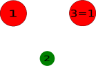
Figure 1: Visual illustration of the numbering convention used to calculate the adiabatic potentials. Particle $2$ is distinctly different from the identical particles $1$ and $3$.

For the simplest case of 3 identical bosons, Eq.(6) reduces to $(M_{11}-M_{12})(M_{11}+2M_{12})=0$, where we only have to distinguish between diagonal and non-diagonal terms. The second factor equal to zero is equivalent to the well-known equation for $\nu(\rho)$ Fedorov2003 ; Braaten2006

$$\nu\cos\left(\frac{\nu\pi}{2}\right)-\frac{8}{\sqrt{3}}\sin(\frac{\nu\pi}{6})=\frac{\rho}{\sqrt{\mu}a}\sin\left(\frac{\nu\pi}{2}\right)\;,$$ (10)

where all indices are omitted for this case of identical bosons. The other case of interest is two identical and one distinguishable particle. We label as illustrated in fig. 1, that is particles 1 and 3 are identical ($m_{1}=m_{3}$, $a_{12}=a_{23}$, $M_{12}=M_{23}$, and $M_{11}=M_{33}$, $M_{13}\neq M_{11}$). The characteristic equation then reduces to

$$(M_{11}-M_{13})(M_{11}M_{22}-2M_{12}^{2}+M_{22}M_{13})=0\;,$$ (11)

where the last factor provides the general physical solution, which receives contributions from all three interacting pairs. Non-interacting particles $1$ and $3$ correspond to vanishing scattering length, $a_{13}=0$, where only two interactions contribute. Then $M_{22}\rightarrow\infty$ and the second factor in Eq.(11) reduces to $M_{11}+M_{13}=0$, which explicitly amounts to

$$\nu\cos\left(\frac{\nu\pi}{2}\right)+\frac{2\sin(\nu[\phi_{13}-\frac{\pi}{2}])}{\sin(2\phi_{13})}=\frac{\rho}{\sqrt{\mu_{1}}a_{12}}\sin\left(\frac{\nu\pi}{2}\right).$$ (12)

In all the calculations of $\nu(\rho)$ we only use the smallest non-trivial solution to the Eqs.(10), (11) and (12). This selects the lowest adiabatic potential in the hyper-spherical expansion. The results obtained for $\nu$ depends on the ratios of hyper-radius to the different scattering lengths.

When $a_{i}\rightarrow\infty$ the purely imaginary solutions, $\nu=\nu_{0}$, become independent of $\rho$, where $\nu_{0}$ depends on the masses and the number of contributing interactions. The radial equation in Eq.(5) has then infinitely many bound solutions, the Efimov three-body states, with energies, $E_{n}$, related by

$$\frac{E_{n+1}}{E_{n}}=e^{-2\pi/|\nu_{0}|}\equiv\frac{1}{s^{2}},$$ (13)

where we generally refer to $s$ as the Efimov scaling. We emphasize that $s$ in particular depends on the number of contributing subsystems. In practical comparison with measurements this means that we can expect $s$ to take any value between the values of the two extreme limits of two or three contributing subsystems.

II.2 Optical potential

We are interested in modelling the recombination for negative values of all the scattering lengths, that is in the regime where no two-body bound states exist within the present zero-range model. We therefore need to introduce the final dimer states populated in the final state of the three-body recombination process. However, the only information we need is the rate of population, or equivalently the rate at which the three-body system disappears. No details of the final states are required, and the optical model is perfect for this purpose sie87 . This model has recently been employed to describe three-body recombination of identical bosons Peder2013 .

We add an imaginary part to the adiabatic hyper-radial potential in Eq.(5) leading to non-hermiticity and non-conservation of probability. Thus we can describe the time-dependent probability reduction as an absorption process, since recombination is removal of probability from the initial three-body system. This is then directly aiming for calculation of the absorption rate. The recombination process occurs when all three particles simultaneously are close in space and two can merge into a dimer, while the third is necessary to conserve energy and momentum. The hyper-radius is an appropriate and convenient measure of average distance between the three particles, see Eq.(1). We therefore modify the potential in Eq.(5) at small distances, $\rho<\rho_{cut}$, by

$$\frac{2m}{\hbar^{2}}V(\rho)=\begin{cases}\frac{\nu^{2}(\rho)-\frac{1}{4}}{\rho^{2}}&\text{if $\rho>\rho_{cut}$}\\ \frac{\nu^{2}(\rho_{cut})-\frac{1}{4}}{\rho_{cut}^{2}}-V_{imag}\cdot i&\text{if $\rho\leq\rho_{cut}$}\end{cases},$$ (14)

where $\rho_{cut}$ and $V_{imag}$ are constants characterizing the optical potential, $V(\rho)$. This structure regularizes the otherwise diverging, for $\rho\rightarrow 0$, real part of the potential by using a $\rho$-independent constant for $\rho<\rho_{cut}$.

The solution, $f(\rho)$, to Eq.(5) is that of a complex square well for $\rho\leq\rho_{cut}$, that is

$$f(\rho)=A\sin(\kappa\rho)\;\;\;\;,\;\;\;\;\kappa=\sqrt{2m(E-V(\rho_{cut}))/\hbar^{2}},$$ (15)

where both $\kappa$ and $V$ are complex quantities. This solution can conveniently be used as initial condition in the numerical solution for an integration starting in $\rho_{cut}$.

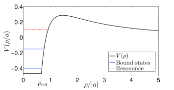
Figure 2: A schematic illustration of the real part of the optical potential for three identical bosons. Both axes use natural length and energy units of $a$ and $\hbar^{2}/(2ma^{2})$. For values $\rho>\rho_{cut}$ it corresponds to the adiabatic potential for identical bosons. At smaller $\rho$ it has a constant real value corresponding to the value of the adiabatic potential in $\rho_{cut}$. The blue lines correspond to some of the bound states of the $-1/\rho^{2}$ potential. The dotted red line illustrates a possible resonant state at positive energy. The scale of this illustration is unphysical, since the value of $\rho_{cut}$ in actual calculations tends to be much smaller relative to the value of $\rho$ where the potential has a maximum.

A schematic illustration of the real part of the potential is shown for three identical bosons on fig. 2. This potential has a short-distance attractive region, a barrier of height $0.287\hbar^{2}/(2ma^{2})$ located at $\rho=1.46a$, and a decrease towards zero as $15/(4\rho^{2})$, where the latter can be seen from Eq.(5) with $\nu=2$ obtained from Eq.(10), since $\sin(\nu\pi/2)=0$ in the limit of $\rho\rightarrow\infty$.

The small distance attractive behavior outside $\rho_{cut}$, but inside the barrier, is proportional to $-1/\rho^{2}$. Such a potential produces a number of bound three-body states, which only is limited by the finite value of $V$ for $\rho<\rho_{cut}$. The energies of these states are related through the scaling in Eq.(13). Physically we can think of the recombination process as related to the probability of reaching the absorptive small distances by tunneling through the barrier. The recombination probability is then substantially enhanced when one of these states has an energy equal to the total three-body energy.

The scattering length is decisive for potential and bound state energies. In particular, for three identical bosons we define $a^{(-)}$ as the value for which a bound state appears with zero energy. The recombination probability consequently peaks for the same, very small, energy close to zero when $a=a^{(-)}$. The parameter $\rho_{cut}$ turns out to determine the value $a^{(-)}$, whereas the strength parameter $V_{imag}$ determines the shape and size of this recombination peak as a function of $a$.

III Three-body recombination

The potential described in the previous section now has to be used to calculate the rate of probability disappearing in the different three-body channels. We first define formally the different channels and rates, then we describe how to compute these rates, first by the traditional method employed for identical particles, and in the last subsection we discuss a new method intuitively related to the optical model.

III.1 Rate equations

For mass-imbalanced recombination the rate equations for the loss-rates are more complicated than for the mass-balanced case. For two components with densities $n_{1}$ and $n_{2}$, we can have three-body systems with one distinguishable and two identical particles. In total we then have 4 different possible recombination processes, and we can in principle find the time derivative of either of the two particle densities which leads to 6 different recombination coefficients, denoted $\alpha$, that is

$$\dot{n_{1}}=-\alpha_{111}^{(1)}n_{1}^{3}-\alpha_{112}^{(1)}n_{2}n_{1}^{2}-\alpha_{221}^{(1)}n_{2}^{2}n_{1},$$ (16)

$$\dot{n_{2}}=-\alpha_{222}^{(2)}n_{2}^{3}-\alpha_{112}^{(2)}n_{2}n_{1}^{2}-\alpha_{221}^{(2)}n_{2}^{2}n_{1}.$$ (17)

Here the indices 1 and 2 refer to the two different kinds of particles in a two-component gas. The first term in Eqs.(16) and (17) corresponds to the recombination coefficient for identical particles, whereas the last two terms correspond to the two mass-imbalanced recombinations.

We shall in the following formal derivations often imagine the example of a Cs-Li gas where Cs is particle 1 and Li particle 2. Then $\alpha_{112}^{(1)}$ corresponds to the recombination process between two particles of type 1 and one particle of type 2, and the rate relates to the change in the particle density of type 1. Analogously for other sub- and superscripts.

The rate equations only describe how many particles disappear from a three-body system. The final state is not specified. We could attempt to further split the mass-imbalanced recombinations into two types depending on the final structure of which particles form the dimer, that is

$$1+1+2\rightarrow 1+(12)\;\;\;\;\;\;\;\text{or}\;\;\;\;\;\;\;1+1+2\rightarrow(11)+2.$$

However, the optical model does not allow distinction between final states, and there is also currently no way to distinguish the two channels experimentally. Thus, $\alpha_{ijk}^{(i)}$ is the full recombination coefficient corresponding to the sum of these different dimer productions.

It is obviously much more difficult to find $n_{1}(t)$ and $n_{2}(t)$ from Eqs.(16) and (17) than solving one much simpler equation corresponding to a gas of identical bosons. However, we assume the coefficients $\alpha_{ijk}^{(i)}$ are density and time-independent, and we are able to calculate these coefficients directly from the radial equation in the optical model-modified Eq.(5). Also experimental analyses are more direct by measuring the loss of individual particles as function of time.

We therefore do not attempt to find the full time dependence from Eqs.(16) and (17). It is, however, reassuring to estimate the time-scale at which the numerically computed values of $\alpha_{ijk}^{(i)}$ make sense. Let us first assume that we have a single-species gas corresponding to the equation $\dot{n_{1}}=-\alpha_{111}^{(1)}n_{1}^{3}$. The solution is

$$\frac{n_{1}(t)}{n_{1}(t_{0})}=\frac{1}{\sqrt{1+2\alpha_{111}^{(1)}n^{2}_{1}(t_{0})(t-t_{0})}}.$$ (18)

This square root dependence holds for the single-species gas. With typical experimental parameters for the density Huang2014 , we find that $n_{1}$ is reduced by a factor of $2$ over a time period varying from about half a second to a few nanoseconds as the scattering length changes from -100$a_{0}$ to -20000$a_{0}$, where $a_{0}$ is the Bohr radius. We used here the values of $\alpha_{111}^{(1)}$ obtained in the calculations reported in details in a later section of this paper.

Let us then consider Eq.(16) but with $n_{2}$ varying slowly enough to assume it is constant. If now the $\alpha_{112}^{(1)}$ recombination is dominant, we get the solution

$$\frac{n_{1}(t)}{n_{1}(t_{0})}=\frac{1}{1+\alpha_{112}^{(1)}n_{1}(t_{0})n_{2}(t_{0})(t-t_{0})}.$$ (19)

Under these assumptions, we get a half-life ranging from a few milliseconds to a few nanoseconds as the $a_{12}$ scattering length grows from -100$a_{0}$ to -10000$a_{0}$. These numbers correspond to a Cs-Li gas, where the densities are obtained from the experiment pires2014 and the values of $\alpha_{112}^{(1)}$ are from calculations reported later in this paper.

If the last term is dominating in Eq.(16) we get analogously an exponential time dependence, that is

$$\frac{n_{1}(t)}{n_{1}(t_{0})}=\exp(-\alpha_{221}^{(1)}n^{2}_{2}(t_{0})(t-t_{0})).$$ (20)

Using the densities obtained from the experiment pires2014 , this half-life ranges from about 150 seconds to a few milliseconds as the $a_{12}$ scattering length increase from about -100$a_{0}$ to -10000$a_{0}$. The relatively large half-life here reflects the small values of $\alpha_{221}^{(1)}$, which are from calculations reported later in this paper.

We shall return with more discussion on calculated values and relative sizes of the recombination coefficients in Eqs.(16) and (17). In general, our results for the rate coefficients, $\alpha_{ijk}^{(i)}$, combined with our simple approximate solutions give realistic time-scales compared to experimental conditions. When analysing the data in a given experiment, a variety of methods are used. Some involve a numerical solution of an equation similar to Eq.(16) pires2014 , while some are more elaborate taking the experimental variation of the temperature with time into account Roy2013 .

In theoretical calculations we generally find the probability loss per unit time for a single three-body system, denoted $J_{ijk}$, which will be refereed to as the recombination rate. From this the probability loss of single particles involved in the recombination can be found. Let us look at the particle loss, corresponding to the terms in Eq.(16). The number of particles $1$ lost per unit time, $\dot{N_{1}}$, from one three-body system is respectively $3J$, $2J$ and $1J$ for the (1-1-1), (1-1-2) and (2-2-1) systems. The total number of three-body systems is respectively $\frac{N_{1}^{3}}{3!}$, $\frac{N_{1}^{2}N_{2}}{2}$ and $\frac{N_{1}N_{2}^{2}}{2}$ for the (1-1-1), (1-1-2) and (2-2-1) systems. Equivalent arguments hold for Eq.(17) and thus we find the total particle loss per unit time to be

$$\dot{N_{1}} = -\frac{3}{3!}J_{111}N_{1}^{3}-\frac{2}{2}J_{112}N_{1}^{2}N_{2}-\frac{1}{2}J_{221}N_{1}N_{2}^{2}$$ (21)

$$\dot{N_{2}} = -\frac{3}{3!}J_{222}N_{2}^{3}-\frac{2}{2}J_{221}N_{2}^{2}N_{1}-\frac{1}{2}J_{112}N_{2}N_{1}^{2}.$$ (22)

The values $J_{ijk}$ depend on the volume in which the three-body systems are confined, and to obtain the $\alpha_{ijk}^{(i)}$ coefficients, we need to transform to densities using the identity $n_{i}=\frac{N_{i}}{V_{i}}$. By insertion of this in Eqs.(21,22) and comparison with Eqs.(16,17) this yields the following relation between recombination rates and recombination coefficients:

$$\alpha_{111}^{(1)}=\frac{1}{2}J_{111}V_{111}^{2}\;\;\;\;\;\;\;,\;\;\;\;\;\;\;\alpha_{222}^{(2)}=\frac{1}{2}J_{222}V_{222}^{2}$$ (23)

$$\alpha_{112}^{(1)}=J_{112}V_{112}^{2}\;\;\;\;\;\;\;,\;\;\;\;\;\;\;\alpha_{112}^{(2)}=\frac{1}{2}J_{112}V_{112}^{2}$$ (24)

$$\alpha_{221}^{(1)}=\frac{1}{2}\ J_{221}V_{221}^{2}\;\;\;\;\;\;\;,\;\;\;\;\;\;\;\alpha_{221}^{(2)}=J_{221}V_{221}^{2}\;.$$ (25)

The indices are necessary to distinguish between the four different three-body systems. The quantity $V_{ijk}^{2}J_{ijk}$, is then independent of the volume, under the assumption that the volume is sufficiently large. The volume used in theoretical calculations and the volume corresponding to specific experiments are not the same, but $V_{ijk}^{2}J_{ijk}$ should be the same and thus it is the quantity for which comparisons between experiment and theory is meaningful. The difference between $V_{ijk}^{2}J_{ijk}$ and the recombination coefficients is the factors related to the number of three-body systems and particles lost per three-body recombination, all of which have been accounted for in Eq.(23)-Eq.(25). For a non-BEC gas there is also a multiplicative symmetry-factor corresponding to the number of particle permutations $P_{ijk}$, as described in Greene2009 , but for a BEC-gas this symmetry factor disappears Kagan1985 ; Greene2009 . For three identical particles $P_{iii}=3!$, while for two identical particles and one distinguishable particle $P_{iij}=2!$.

In the following two sections, two methods of calculating $J_{ijk}$ for any three-body system is derived. In order to ease the notation the subscripts on $J$ and $V$ are omitted.

III.2 S-matrix method

The recombination rate $J$ for a given three-body system is defined from the missing probability after scattering on the optical potential in Eq.(14). Let us assume the three-body wave-function asymptotically is expressed in Jacobi coordinates as a three-dimensional plane wave normalized in a box of volume, $V$. We expand this wavefunction in hyper-harmonic free solutions, that is Garrido2014

$$\psi=\frac{1}{V}e^{i\mathbf{k_{x}}\mathbf{x}+i\mathbf{k_{y}}\mathbf{y}}=$$

$$\frac{1}{V}\frac{(2\pi)^{3}}{(\kappa\rho)^{2}}\sum_{\mathcal{K}}i^{K}\mathcal{Y}^{\ast}_{\mathcal{K}}(\Omega_{\kappa})\mathcal{Y}_{\mathcal{K}}(\Omega_{\rho})J_{K+2}(\kappa\rho),$$ (26)

where $\mathbf{k_{x}}$ and $\mathbf{k_{y}}$ are the Jacobi momenta characterizing the wave function, $\kappa^{2}=(k_{x}^{2}+k_{y}^{2})$, and $\Omega_{\kappa}$ denote the five hyper-angles associated with the directions of $\mathbf{k_{x}}$ and $\mathbf{k_{y}}$. The three-body energy is then defined by

$$E=\frac{\hbar^{2}\kappa^{2}}{2m}.$$ (27)

The arguments of the two hyperspherical harmonics, $\mathcal{Y}_{\mathcal{K}}$, are related to the spatial and momentum coordinates, respectively. The collection of angular quantum numbers are denoted $\mathcal{K}$, where we only need to specify the hyper-momentum quantum number, $K$. The kinetic energy eigenvalue corresponding to the free wave-function is $K(K+4)$ and at asymptotically large values of $\rho$ related to the eigenvalue of the adiabatic potentials as $K=\nu(\rho\rightarrow\infty)-2$. The asymptotic value of $\nu$ for the lowest adiabatic potential is 2, corresponding to $K=0$.

The radial dependence is given in terms of the spherical Bessel function, $J_{K+2}$, of order $K+2$. The hyper-harmonics are normalized to unity

$$\int d\Omega\mathcal{Y}^{\ast}_{\mathcal{K}^{\prime}}\mathcal{Y}_{\mathcal{K}}=\delta_{\mathcal{K}^{\prime}\mathcal{K}},$$ (28)

where the delta-function express that all quantum numbers pairwise must be equal. The large-distance asymptotics, $\rho\rightarrow\infty$, is then obtained from the Bessel function, that is Abramowitz

$$J_{K+2}(\kappa\rho)\xrightarrow[\rho\to\infty]{}\sqrt{\frac{2}{\pi\kappa\rho}}\frac{e^{i\kappa\rho-i\varphi_{K}}+e^{-i\kappa\rho+i\varphi_{K}}}{2},$$ (29)

where $\varphi_{K}=(K+2)\frac{\pi}{2}-\frac{\pi}{4}$. The two terms in Eq.(29) correspond to in- and out-going hyper-sperical waves, respectively. We now introduce a short-range optical potential and a unit amplitude on the in-coming wave. The absolute value of the out-going amplitude is then asymptotically allowed to differ from unity. From Eqs.(26) and (29) we then obtain the asymptotic from the $K=0$ wave function, that is

$$\frac{1}{V}\frac{(2\pi)^{3}}{(\kappa\rho)^{2}}\mathcal{Y}^{\ast}_{0}(\Omega_{\kappa})\mathcal{Y}_{0}(\Omega_{\rho})\sqrt{\frac{2}{\pi\kappa\rho}}\frac{S_{11}e^{i\kappa\rho-i\varphi_{0}}+e^{-i\kappa\rho+i\varphi_{0}}}{2},$$ (30)

where $0<|S_{11}|<1$, since the optical potential acts as a sink of probability. The hyper-radial current is defined by

$$j_{\rho}=-i\frac{\hbar}{2m}\left(\psi^{\ast}\frac{\partial}{\partial\rho}\psi-\frac{\partial}{\partial\rho}\psi^{\ast}\psi\right).$$ (31)

Using Eqs.(30) and (31) the missing current, $\Delta j_{\rho}=j_{\rho}(S_{11}=1)-j_{\rho}(S_{11})$, is calculated for a given value of $S_{11}$. This amounts to

$$\Delta j_{\rho}=\frac{1}{V^{2}}\frac{\hbar}{m}\kappa\left(\frac{2\pi}{\kappa\rho}\right)^{5}(1-|S_{11}|^{2})|\mathcal{Y}^{\ast}_{0}(\Omega_{\kappa})\mathcal{Y}_{0}(\Omega_{\rho})|^{2}.$$ (32)

To get the probability loss per unit time, $J$, we need to integrate the missing current over the hyper-surface. The surface element must correspond to the physical volume element (see Garrido2014 ). The volume element is thus given by (see Eqs.(2) and (3)):

$$d^{3}\mathbf{r_{x}}d^{3}\mathbf{r_{y}}=\left(\frac{1}{{\mu}_{i}{\mu}_{jk}}\right)^{3/2}d^{3}\mathbf{x}d^{3}\mathbf{y}=$$

$$m^{3}\big{(}\frac{m_{i}+m_{j}+m_{k}}{m_{i}m_{j}m_{k}}\big{)}^{3/2}\rho^{5}d\rho d\Omega_{\rho},$$ (33)

where we do not have to distinguish between choice of Jacobi coordinates, since the mass factor is symmetric under exchange of $i$, $j$ and $k$. To take into account the degeneracy of the initial states for a given $\kappa$ we need to average over $\Omega_{\kappa}$, which we do by integrating over the angles and dividing by $\int d\Omega_{\kappa}=\Omega_{5}=\pi^{3}$. For a given $\kappa$ (or energy) , and under the assumption that we are at large values of $\rho$, we then get

$$J=\int m^{3}\big{(}\frac{m_{i}+m_{j}+m_{k}}{m_{i}m_{j}m_{k}}\big{)}^{3/2}\frac{d\Omega_{\kappa}}{\Omega_{5}}\rho^{5}d\Omega_{\rho}\Delta j_{\rho}.$$ (34)

Exploiting the orthonormality of the hyperspherical harmonics, the missing probability per unit time is then

$$J=m^{3}\big{(}\frac{m_{i}+m_{j}+m_{k}}{m_{i}m_{j}m_{k}}\big{)}^{3/2}\frac{1}{\Omega_{5}}\frac{\hbar\kappa}{{m}}\left(\frac{2\pi}{\kappa}\right)^{5}(1-|S_{11}|^{2})\frac{1}{V^{2}}.$$ (35)

In order to obtain the recombination coefficients we must multiply by $V^{2}$. This gives

$$JV^{2}=m^{3}\big{(}\frac{m_{i}+m_{j}+m_{k}}{m_{i}m_{j}m_{k}}\big{)}^{3/2}8\pi^{2}\frac{\hbar^{5}}{m^{3}}\frac{(1-|S_{11}|^{2})}{E^{2}},$$ (36)

which corresponds to the general formula for N-body loss given in Greene2009 .

III.3 Decay-rate method

In this section we present an alternate way to obtain the recombination rate $J$ for the three-body system. This is done by deriving the decay rate of bound states in the optical potential. First we define the bound states in a large box with hyper-radius extending from zero to $\rho_{max}$. The boundary condition is that the wave function is zero at the edge of the box, that is $f(\rho_{max})=0$. The eigenvalues for the optical potential are complex numbers

$$E=E_{0}-\frac{1}{2}i\Gamma.$$ (37)

The imaginary component of the energy describes the decay rate of the probability as seen from the time evolution of the wave-function, defined by

$$|f(\rho,t)|^{2}=|f(\rho,t=0)|^{2}\exp(-\Gamma t/\hbar).$$

The decay rates described by $\Gamma=J\hbar$ are three-body energies determined by a box boundary condition. The overall energy dependence is then a strong decrease, inversely proportional to the hyper-radial three-body volume, towards zero as function of box radius $\rho_{max}$. In order to obtain the recombination coefficient $\frac{\Gamma}{\hbar}V^{2}$ we then need to know $V$. This volume, $V$, is defined by equating two ways of calculating the density of three-body states in the hyper-spherical box extending to $\rho_{max}$. The first is the formal expression of integration over given intervals of coordinates and conjugate momenta, where $\mathbf{p_{x}}=\hbar\mathbf{k_{x}}$ and $\mathbf{p_{y}}=\hbar\mathbf{k_{y}}$. The second is direct numerical calculation of the same quantity from the solutions to the hyper-radial equation. The resulting equation is then

$$\int d^{3}\mathbf{x}d^{3}\mathbf{y}d^{3}\mathbf{p_{x}}d^{3}\mathbf{p_{y}}\delta(E-(p_{x}^{2}+p_{y}^{2})/(2m))=$$

$$V^{\prime 2}\Omega_{5}\hbar^{6}\kappa^{5}d\kappa/dE=(2\pi\hbar)^{6}d\nu/dE\;$$ (38)

where $V^{\prime 2}=\int d^{3}\mathbf{x}d^{3}\mathbf{y}$ is the volume for the Jacobi coordinates, $\Omega_{5}\kappa^{5}d\kappa/dE$ is the volume element per unit energy in momentum space, and $d\nu/dE$ is the density of states for a given energy, $E$, defined by Eq.(27). The factor $2\pi\hbar=h$ is Plancks constant, which is the volume occupied by each quantum state.

Using Eq.(33) we express $V^{\prime}$ in terms of the physical volume, $V$, that is

$$V^{2}=\int d^{3}\mathbf{r_{x}}d^{3}\mathbf{r_{y}}=V^{\prime 2}m^{3}\big{(}\frac{m_{i}+m_{j}+m_{k}}{m_{i}m_{j}m_{k}}\big{)}^{3/2}\;.$$ (39)

Using Eqs.(38), (27) and (39) we then get

$$V^{2}=m^{3}\big{(}\frac{m_{i}+m_{j}+m_{k}}{m_{i}m_{j}m_{k}}\big{)}^{3/2}\frac{1}{E^{2}}\frac{d\nu}{dE}\frac{2}{\Omega_{5}}\left(\frac{\hbar^{2}(2\pi)^{2}}{2m}\right)^{3}\;,$$ (40)

where the value of $\frac{d\nu}{dE}$ can be found from solving the hyper-radial equation numerically.

We emphasize that the lowest hyper-radial equation only accounts for both total and partial-wave angular momentum zero states, while the employed phase-space identity includes all states, independent of angular momentum. The derived relations therefore strongly assume excitation energies sufficiently small to exclude contributions from all solutions build on the repulsive higher-lying adiabatic potentials.

The squared volume $V^{2}$ scales as $V^{2}\propto\rho_{max}^{6}$, and meaningful recombination coefficients, independent of box size, are therefore only achieved when $\Gamma$ is proportional to $\rho_{max}^{-6}$. This is very demanding for numerical calculations, since convergence only is achieved when $\rho_{max}$ is larger than the scattering lengths.

The recombination coefficients, expressed in terms of $\Gamma$, are then found from

$$JV^{2}=m^{3}\big{(}\frac{m_{i}+m_{j}+m_{k}}{m_{i}m_{j}m_{k}}\big{)}^{3/2}16\pi^{3}\frac{\hbar^{5}}{m^{3}}\frac{1}{E^{2}}\frac{d\nu}{dE}\Gamma.$$ (41)

Eq.(41) is equal to Eq.(36) then. This leads to the immediate conclusion that for an energy $E$ corresponding to an allowed eigenvalue the following relation between the parameters in the two methods should hold

$$\Gamma=\frac{1}{2\pi}\frac{dE}{d\nu}(1-|S_{11}|^{2}).$$ (42)

III.4 Recombination coefficients and finite temperature

One immediate conclusion which is readily obtained from Eq.(23)- Eq.(25)is that

$$\alpha_{112}^{(2)}=\frac{1}{2}\alpha_{112}^{(1)}\;,\;\alpha_{221}^{(2)}=2\alpha_{221}^{(1)}\;,$$ (43)

which is reassuring, as for example one particle of type 2 disappears for each particle of type 1 in the 1-1-2 recombination. For identical particles the mass factor in $JV^{2}$ (Eq.(36) and Eq.(41)) reduces to $\frac{1}{m_{i}^{3}}$, where $m_{i}$ is the physical mass. Numerically, we find that the tunnelling probability $1-|S_{11}|^{2}$ (for an analytical estimate of this, see pks2013 ; Sorensen2013 ) and the decay rate $\Gamma$ depends on the physical mass as $m_{i}^{2}$, however, leading to the identity $\alpha_{111}^{(1)}\approx\frac{m_{2}}{m_{1}}\alpha_{222}^{(2)}$. It is approximate since the Efimov peaks can have different locations and shapes in the two systems, leading to non-systematic differences between $\Gamma$ or equivalently $S_{11}$ in the two systems. This mass-dependence for identical bosons is in correspondence with earlier work Nielsen1999 .

In order to compare our calculations with experimental data we need to fold our calculated values of $\alpha_{ijk}^{(i)}(E)$ with a temperature distribution. The normalised Boltzmann distribution for 3 particles is given by Peder2013

$$\langle\alpha_{ijk}^{(i)}\rangle_{T}=\frac{1}{2(k_{B}T)^{3}}\int E^{2}e^{-\frac{E}{k_{b}T}}\alpha_{ijk}^{(i)}(a,E)dE\;,$$ (44)

where the $E^{2}$ factor arises from the three-body phase-space. In order to get good results it is necessary to calculate $\alpha_{ijk}^{(i)}$ in a range of energies around $k_{b}T$, where the integral receives contributions.

The highest excitation energies allowed in our low-energy model are given by the energy difference between states build on the first and the neglected second and higher adiabatic potentials. This energy difference can be estimated by the difference in potential energies at distances where the states are located. Since the scattering length is a measure of the sizes of all these Efimov-like states, we use the hyper-radius $\rho\approx 10^{4}a_{0}$ to give a lower estimate of the maximum temperature allowed in realistic calculations. The energy difference between first and second adibatic potential is for interaction free states given by $\hbar^{2}K(K+4)/(2m\rho^{2})$ where $K=2$ nie01 . The result of these estimates are temperatures of the order of $\approx 1\mu K$, which therefore is an upper temperature limit for realistic calculations.

With the temperature distribution implemented by Eq.(44) the two methods, that is the S-matrix and the the decay rate, give essentially the same results for the same choice of $\rho_{cut}$ and $V_{imag}$, aside from numerical inaccuracies. We shall use whichever method is the most convenient in the practical calculations. For technical reasons it is for example generally more convenient to implement the zero-energy limit by the decay rate method, while it is easier to implement the temperature distribution for the S-matrix method.

IV Parameter dependence

The recombination coefficients for our two-component system depend on three parameters, that is one mass ratio and two scattering lengths. We use the notation from fig. 1 where the particles 1 and 3 are identical, and 2 is distinctly different. To illustrate the effects we investigate first the variation of the adiabatic potential which is the crucial ingredient in all the calculations. Before we investigate the dependence of the recombination on physical parameters, we investigate the dependence on the optical model parameters. Then we investigate the dependence on scattering lengths for masses of systems where experimental results are available. Finally we compare the different recombinations that can occur in a two-component gas. The factors corresponding to a non-BEC gas are used for all the recombination coefficients.

The numerical calculations are technically simple and employ only homemade standard programs. First the lowest adiabatic potential is found numerically from the complex angular eigenvalues, which in tur is found by solving Eq.(6). The absorption probability is then calculated for different energies from the probability reduction of a plane wave reflected by the optical model potential. This involves solving Eq.(5), at a given energy, for the modified potential Eq.(14). This is done by numerical integration with initial conditions in $\rho_{cut}$ provided by Eq.(15). The result are then fitted to Eq.(30) in order to extract $S_{11}$. The complex eigenvalue of the optical potential is calculated by the shooting method, by requiring that the wave-function is zero at $\rho_{max}$. The numerical integration is implemented as in the above $S$-matrix calculations.

IV.1 Adiabatic potentials

The masses only enter as ratios of masses through the $\phi_{ij}$ functions in Eq.(9), that is for our case this leaves only one parameter, $R=\frac{m_{1}}{m_{2}}$. We show computed mass dependence of adiabatic potentials in fig. 3 as functions of hyper-radius measured in units of the scattering length, $a_{12}$ of the distinguishable particles. The two figures show results for a vanishing and a relatively large scattering length between the identical particles $a_{11}$. We see that all potentials asymptotically approach $\frac{15/4}{\rho^{2}}$, as in the case of identical particles.

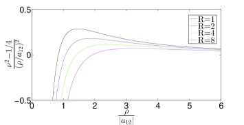
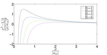
Figure 3: The lowest adiabatic potentials as function of $\rho/a_{12}$, calculated from Eqs.(12) and (11). The lower figure is for $a_{11}=0$ and the upper figure is for $a_{11}=a_{12}$.

For both values of $a_{11}$ we find that increasing $R$ leads to lower barrier height, and a shift to smaller hyper-radii of barrier position and $\rho$-value, where the potential is zero. The dependence is strongest for two heavy and one light particle, that is for $R>1$. Continuing to $R<1$ would give very little variation in the potentials compared to the $R=1$ curve. Increasing $|a_{11}|$ from zero reduces the peak heights and move the potentials towards larger hyper-radii.

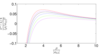
Figure 4: The lowest adiabatic potentials as function of $\rho/a_{12}$. The red graph corresponds to Eq.(12). The other graphs, in descending order, corresponds to $a_{11}=0.08,0.16,0.32,0.64,1.28a_{12}$ where $a_{12}$ is negative, calculated from Eq.(11).

Experimental data are available for a Cs-Li gas where the mass ratio is $R=22.28$. The dependence on the scattering length, $a_{12}$, is shown in fig. 4 for different values of $a_{11}$. The potential is rather small for this value of $R$, but still with a distinct barrier where the height decreases with increasing values of $|a_{11}|$.

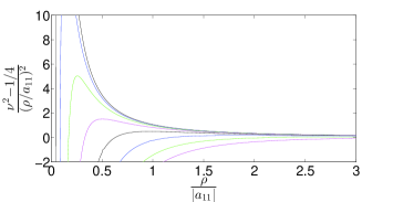
Figure 5: The lowest adiabatic potentials as function of $\rho/a_{11}$. These graphs, in descending order, corresponds to $a_{12}=0.01,0.02,0.04,0.08,0.16,0.32,0.64,1.28a_{11}$ where $a_{11}$ is negative, calculated from Eq.(11).

To complement we show the dependence on $a_{11}$ in fig. 5 for different values of $a_{12}$. The barrier decreases with increasing $a_{12}/a_{11}$ from a rather large value for vanishing $|a_{12}|$, towards rather small values. For large values of $|a_{12}|$ the barrier has become so small and moved so far to the right, that it is no longer visible on the scale chosen for the figure.

These figures show that increasing $|a_{11}|$ and $|a_{12}|$ has the same qualitative effect as increasing the scattering length in the case of identical bosons for the optical model, see fig. 2. It decreases the height of the barrier and moves the location of its maximum to the right.

IV.2 Optical model

The real potential is completely determined for zero-range two-body interactions in terms of scattering lengths and masses. The box-like imaginary potential has hyper-radius and strength as the two phenomenological parameters. This radius can only assume discrete values determined by the requirement that the scattering length is reproduced for the occurrence of a specific recombination peak. The corresponding strength correlatedly varies shape and size of the chosen peak. On fig. 6 the results of varying $V_{imag}$, while $\rho_{cut}$ is a constant value of $1.4a_{0}$ are shown.

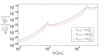
Figure 6: The recombination coefficient for Cs-Cs-Cs as function of the scattering length $a$ for different choices of $V_{imag}$, at $\rho_{cut}=1.4a_{0}$

We see that increasing the size of $V_{imag}$ makes the peaks more pronounced while also making the absolute value for the rest of the graph somewhat smaller. Decreasing the size of $V_{imag}$ has the opposite effect. This is the exact same qualitative effect which was seen when varying the absorption parameter $n_{*}$ describing deeply bound states in Hammer2010 .

From one set of parameters another equally good choice is found by scaling the square well hyper-radius up or down by the Efimov factor and at the same time scaling the strength in opposite direction by the square of the same Efimov factor. Using these parameters reproduces exactly the same shape of the Efimov resonance and the same absolute value of the recombination. This means that $V_{imag}\rho_{cut}^{2}$ for a given peak has a constant value where $\rho_{cut}$ can discretely vary by the Efimov factor. The largest allowed hyper-radius must be at a hyper-radius where the real potential precisely has the inverse radial square behavior. The lowest value is only limited by the requirement that it must be finite, since otherwise the already removed zero-range divergency reappears. In practical calculations we generally pick values in the order of $a_{0}$ to be certain that we do not approach any of these limiting cases.

IV.3 Recombination

For identical particles we know that the recombination coefficient is proportional to the fourth power of the scattering length. For a two-component system this relation must be extended to account for two different scattering lengths as well as for a mass-ratio dependence. We shall illustrate with two mass ratios $R=22.2$ and $R=2.23$, corresponding to experimentally realizable systems, that is ⁶Li-¹³³Cs pires2014 ; tung2014 and ³⁹K-⁸⁷Rb gases. We used these isotopes to have well-defined mass ratios in the calculations. The characteristic small mass variations between isotopes would only marginally change the results, provided the boson-fermion characters remain the same or become irrelevant as when only one identical atom participates in the process. Here we shall only investigate the pure mass dependence.

The dominating recombination coefficient is related to $\alpha_{112}^{(1)}=2\alpha_{112}^{(2)}$, where label 2 corresponds to the light particle. This means that we here consider the heavy-heavy-light three-body systems with mass ratios, $R=22.2$ and $R=2.23$. We calculate all the recombination coefficients in the limit of zero three-body energy.

The periodic structure of enhanced recombination occurs each time the scattering length is multiplied by the Efimov scaling factor, $s=\exp(\pi/|\nu(\rho=\infty)|)$, found for infinite scattering lengths of the contributing systems. This scaling parameter depends first of all on the mass ratio. The Efimov effect requires that $|a_{12}|=\infty$, while $|a_{11}|$ can assume any finite or infinite values. The results for the two limiting cases, $|a_{11}|=0$ and $\infty$, are given in table 1 as a function of mass ratio, $R$. For large $R$ the two cases are almost identical, but there is a big difference for small mass-ratios and this trend continues for $R<1$. If all three scattering lengths are infinitely large the scaling for $R=1$ is $s=22.7$ and for small $R$ approaches a constant of $s=15.7$. For a more detailed discussion of the two different cases see Braaten2006 .

Table 1: Efimov scaling factor $s$ for different values of R

$R=\frac{m_{1}}{m_{2}}$	1	2	5	10	15	20
$a_{12}=a_{11}=\infty$	22.7	20.8	13.7	8.50	6.30	5.14
$a_{12}=\infty,a_{11}=0$	1986	153.8	23.3	9.76	6.64	5.25

The influence of $a_{11}$ can conveniently be studied through the recombination of the two chosen systems. For $R=22.2$ the Efimov scaling only varies between 4.8766 for $a_{11}=0$ and 4.7989 for $|a_{11}|=\infty$ and the peak positions should therefore remain. In contrast the scaling between peaks for $R=2.23$ should move between the extreme limits of 121.1 for $a_{11}=0$ and 20.28 for $|a_{11}|=\infty$ as a function of $a_{11}$.

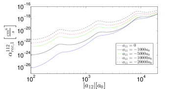
Figure 7: The recombination coefficient, $\alpha_{112}^{(1)}$, as a function of $a_{12}$, for different values of $a_{11}$, where $R=22.2$. The parameters of the optical potential are $V_{imag}=68\frac{\hbar^{2}}{ma_{0}^{2}}$, with $\rho_{cut}$ in the interval, 0.24-0.32$a_{0}$ as $a_{11}$ varies from 0 to -20000$a_{0}$, adjusted to maintain the position of the first Efimov peak at $a_{12}\approx-320a_{0}$.

Let us first focus on the recombination coefficient, $\alpha_{112}^{(1)}$, for a large mass ratio of $22.28$. We calculate $\alpha_{112}^{(1)}$ as a function of $a_{12}$, for different constant values of $a_{11}$. The strength of the optical potential is $V_{imag}=68\frac{\hbar^{2}}{ma_{0}^{2}}$, whereas $\rho_{cut}$ is adjusted slightly to reproduce the peak position $|a_{1}^{(-)}|\approx-320a_{0}$, corresponding to the experimental peak position of Cs-Cs-Li pires2014 ; tung2014 , for the different values of $a_{11}$.

The main results of these calculations are summed up in fig. 7, where we show the coefficient as a function of $a_{12}$ for different values of $a_{11}$. The most striking feature of fig. 7 is that the different values of $a_{11}$ lead to a different overall dependence of $\alpha_{112}^{(1)}$ as function of $a_{12}$. For small values of $|a_{11}|$ there is a $a_{12}^{4}$ dependence corresponding to the $a^{4}$ scaling for identical bosons, but for bigger values of $|a_{11}|$ this relation is no longer valid. As $|a_{11}|$ grows bigger, the recombination is enhanced, which is most visible at smaller values of $|a_{12}|$. This is consistent with larger values of each of the scattering lengths, $|a_{12}|$ and $|a_{12}|$, lowering the potential barrier, making it easier to reach small distances and thereby enhancing the recombination.

We also know that $a_{12}$ has a stronger influence on the potential than $a_{11}$, which corresponds well with $a_{12}$ being the most important parameter for the recombination shown in fig. 7. Specifically, we see that $\alpha_{112}^{(1)}$ changes more as $a_{12}$ runs from 0 to -20000 $a_{0}$, than it does when $a_{11}$ varies from 0 to -20000 $a_{0}$.

All in all, for realistic values of the scattering lengths, we can view $a_{11}$ as moderating the $a_{12}$ dependence and simultaneously enhancing the recombination. More violent changes of $a_{11}$ cannot be excluded when the interactions are controlled by the Feshbach resonance technique. However, this is not the case in any of the physical systems discussed here.

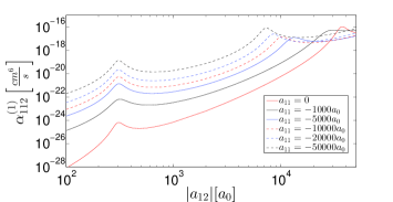
Figure 8: The recombination coefficient, $\alpha_{112}^{(1)}$ as a function of $a_{12}$ calculated for different values of $a_{11}$, where $R=2.23$. The strength of the potential is as in fig. 7 while $\rho_{cut}$ is adjusted to give one peak at about $a_{12}\approx-300a_{0}$.

We now move to the mass ratio $R=2.23$ where the Efimov scaling has a strong dependence on $a_{11}$ as seen from the extreme limits given in table 1. The relative positions of the recombination peaks must then vary with the finite value of $a_{11}$. Again we calculate $\alpha_{112}^{(1)}$ as a function of $a_{12}$ for different values of $a_{11}$. The results of such a series of calculations are shown in fig. 8, where $\rho_{cut}$ is adjusted to produce the same somewhat arbitrary peak position at about $|a_{1}^{(-)}|\approx-300a_{0}$ for all $a_{11}$. The next Efimov peak then has to move in the interval of $a_{12}$ from $20.28\cdot a^{(-)}\approx-6000a_{0}$ and $121.1\cdot a^{(-)}\approx-36000a_{0}$.

Table 2: The ratio, $a_{2}^{(-)}/a_{1}^{(-)}$, between the $a_{12}$ scattering lengths for the first two peaks as function of $a_{11}$ when $R=2.23$. The last column give the related $\rho_{cut}$ values.

$a_{11}$ $[a_{0}]$	0	-1000	-5000	-10000	-20000	-50000
$\frac{a_{2}^{(-)}}{a_{1}^{(-)}}$	119.4	96.9	41.9	32.9	27.7	23.9
$\rho_{cut}[a_{0}]$	1.21	0.97	1.14	1.18	1.2	1.22

The most noticeable thing in fig. 8 is that the location of the second Efimov resonance changes with the finite value of $a_{11}$. This variation of the ratio between $a_{12}$ values of second and first peak is shown in table 2 for different $a_{11}$ values. The rather modest variation of $\rho_{cut}$ is also shown in this table. We notice the correct continuous variation between the two extreme limits of the Efimov scaling with $a_{11}$, although the value of $\rho_{cut}$ for $a_{11}=0$ reflects the singularity moving between Eqs.(10) and (12).

We emphasize that small changes of $\rho_{cut}$ is fine-tuning to maintain the first peak at the same position. The much larger shift of the second peak is entirely due to the variation of $a_{11}$, and essentially completely independent of the parameters of the imaginary potential. A substantial change in the second peak position requires a value of $a_{11}\approx-5000a_{0}$. However, the change is fairly gradual and there is no ”magic value” where $a_{11}$ suddenly begins to contribute. The ideal Efimov scaling for three resonant interactions of 20.28 is essentially reached numerically when $a_{11}=-50000a_{0}$.

The second prominent feature in fig. 8 is that a finite value of $a_{11}$ modifies the overall dependence of $\alpha_{112}^{(1)}$ as a function of $a_{12}$. This is the same qualitative feature as seen in fig. 7 for the large mass ratio $R=22.2$. Finite values of $a_{11}$ leads to a higher absolute value of $\alpha_{112}^{(1)}$ within a huge $a_{12}$ interval, $a_{12}\in[0,-20000a_{0}]$. This means that increasing the size of $|a_{11}|$ enhances the recombination coefficient, like we found for the $R=22.2$ system.

IV.4 Different recombination processes

We have so far only considered recombination from three-body systems with two heavy and one light particle such as Rb-Rb-K and Cs-Cs-Li. However, the same two-component gas can also decay by the other 3 combinations, two light and one heavy particle (Rb-K-K, Cs-Li-Li), and 3 identical heavy (Rb-Rb-Rb, Cs-Cs-Cs) or light particles (K-K-K, Li-Li-Li). In order to estimate the importance of the terms in Eqs.(16) and (17), it is necessary to calculate all these recombination coefficients.

To make a realistic comparison we first consider the Cs-Li gas, where the Efimov resonances are fixed by experimental data for Cs-Cs-Li pires2014 , Cs-Cs-Cs Berninger2011 and Li-Li-Li Dyke2013 , and the parameters of Li-Li-Cs are assumed to be the same as for Cs-Cs-Li. We assume that $a_{11}=a_{22}=0$. This would underestimate the recombination coefficients as shown in the previous subsection, but it allows on the other hand a clean comparison where the fourth power dependence applies, $\alpha_{ijk}^{(1)}\propto a_{12}^{4}$. Actual correlated finite values of these scattering lengths obtained through the Feshbach technique could then be important and quantitatively alter the comparison.

On figure 9 all the recombination coefficients for the Cs-Li gas have been plotted. The optical model parameters are chosen to reproduce the position of the lowest measured recombination peaks pires2014 ; Berninger2011 ; Dyke2013 . The experimental data for Li is actually for ⁷Li Dyke2013 , but our aim is here only to test the mass dependency. In the ¹³³Cs-⁶Li experiment, Li-Li-Li and Li-Li-Cs recombinations are expected to be suppressed due to Fermi statistics, which is not taken into account in our model. So the results are not directly comparable to the experiment. In addition this is not a direct comparison between the mass-balanced and mass-imbalanced case, since the recombination coefficient is a function of different scattering lengths in the different cases.

Furthermore, for $a_{22}=0$ it was not possible to locate an Efimov resonance within the range of $a_{12}\in[0,-10000a_{0}]$ for neither the Li-Li-Cs nor the K-K-Rb mass ratio, even though a wide range of $\rho_{cut}$ were tested. This is because the Efimov scaling factor now is so big that it is hard to locate an interval with even one Efimov resonance. In these comparisons we shall focus on recombination coefficients for zero energy.

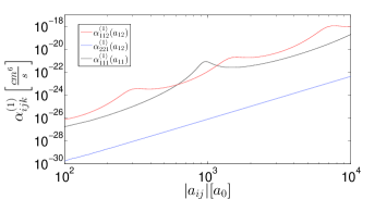
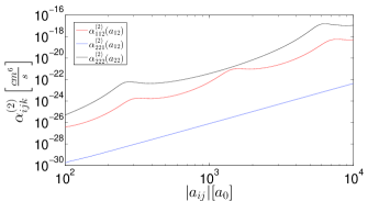
Figure 9: The top shows the recombination coefficients resulting in Cs loss, and the bottom shows the recombination coefficients resulting in Li loss, both as a function of $a_{12}$. The optical parameters in the calculations are $\rho_{cut}=0.20a_{0}$ and $V_{imag}=240\frac{\hbar^{2}}{ma_{0}^{2}}$ is used for Cs-Cs-Li and Li-Li-Cs. For the Cs-Cs-Cs recombination $\rho_{cut}=1.4a_{0}$ and $V_{imag}=16\frac{\hbar^{2}}{ma_{0}^{2}}$ are used and for Li-Li-Li $\rho_{cut}=0.41a_{0}$ and $V_{imag}=68\frac{\hbar^{2}}{ma_{0}^{2}}$ are used.

The absolute sizes on fig. 9 show that the Cs-Cs-Li recombination is much more likely than the Li-Li-Cs recombination for the same value of $a_{12}$. The Cs-Cs-Cs recombination only depends on $a_{11}$, which is used as the $x$-coordinate for this process in fig. 9. This scattering length is expected to be of less importance compared to $a_{12}$ in the mixed recombination coefficients, and therefore assumed to be zero in those estimates.

The comparison is then not straightforward but still useful, since a finite value of $a_{11}$ would increase $\alpha_{112}^{(1)}$ beyond the curve in fig. 9. Thus we deduce that $\alpha_{112}^{(1)}(a_{11}=0,a_{12})\gg\alpha_{111}^{(1)}(a_{11}=a_{12})$, and we therefore believe that the Cs-Cs-Li recombination is much more likely to occur than the Cs-Cs-Cs recombination in realistic systems. We also see in fig. 9 that $\alpha_{222}^{(2)}(a_{22}=a_{12})\gg\alpha_{112}^{(2)}(a_{11}=0,a_{12})$. This does not allow any conjecture about relative sizes in a realistic system because the intra-species scattering lengths usually are much smaller than the necessary large (for the Efimov effect) inter-species scattering length. The recombination coefficients between identical particles are then expected to be relatively small.

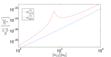
Figure 10: Recombination coefficients for $R=2.23$ as a function of $a_{12}$. The optical parameters are $\rho_{cut}=2.79a_{0}$ and $V_{imag}=20\frac{\hbar^{2}}{ma_{0}^{2}}$ for both systems.

To complement we now investigate the much smaller mass ratio $R=2.23$ (corresponding to a Rb-K gas). The results are shown on fig. 10 for different recombination processes. The optical model parameters are chosen to give a peak for $a_{12}\approx-700a_{0}$ in the $\alpha_{112}^{(1)}$ coefficient. As for the larger mass ratio we again conclude that the heavy-heavy-light recombination process is more likely than the ligt-light-heavy recombination process.

Figs. 9 and 10 also lead to another conclusion. A bigger mass-ratio seems to give a bigger recombination coefficient for two heavy particles and one light. This is in accordance with a corresponding decrease of size of the adiabatic potentials, which intuitively suggests higher probability for recombination at small hyper-radii.

A bigger mass-ratio also seems to give a somewhat smaller recombination coefficient for two light particles and one heavy particle, although not as pronounced. This means that the bigger the mass-ratio, the bigger the difference between the heavy-heavy-light recombination and the light-light-heavy recombination. For both small and big mass-ratios, the $\alpha_{221}^{(i)}$ terms can be neglected in Eqs.(16) and (17) based solely on these mass-related arguments.

We emphasize these conclusions are only strictly valid for small $|a_{11}|$ and $|a_{22}|$. Finite values imply more complicated relations between the different recombination coefficients which only can be determined by taking the Feshbach resonances of a specific system into account. So in theory, it is possible to have a specific system where the light-light scattering length $|a_{22}|$ is much bigger than the heavy-heavy scattering length $|a_{11}|$, which in turn leads to dominance of the light-light-heavy over the heavy-heavy-light process.

V Comparison With Experiment

In this section we will confront our theoretical results with recent experiments that have been carried out for a ¹³³Cs-⁶Li gas pires2014 ; tung2014 , as well as with a recent experiment for a ¹³³Cs gas, in which a second Efimov resonance has been observed Huang2014 . The variable parameter in experiments is the magnetic field $B$, which via the mechanism of Feshbach resonances can be used to change the scattering lengths, $a$. The phenomenological relation between $a$ and $B$ is

$$a(B)=a_{bg}\left(1+\frac{\Delta}{B-B_{0}}\right)$$ (45)

where $\Delta$ , $a_{bg}$ and $B_{0}$ are determined experimentally for each individual system. Eq.(45) applies for most systems and will be used in the cases investigated in this section. We first focus on the equal mass process after which we continue with the dominating heavy-heavy-light recombination process.

V.1 The ¹³³Cs-¹³³Cs-¹³³Cs recombination

Recently a second Efimov resonance was observed in a ¹³³Cs gas Huang2014 , and we can conveniently test the model against this experimental confirmation of the original Efimov scenario. The first Efimov resonance for a ¹³³Cs gas was observed earlier Berninger2011 to have a peak for $a^{(-)}\approx-960a_{0}$. The experimental data from these measurements also allow us to adjust both $\rho_{cut}$ to give the peak position and subsequently tune the strength, $V_{imag}$, to the shape of this first peak. With the scaling mass, $m$, of ¹³³Cs, $\rho_{cut}=1.4a_{0}$ and $V_{imag}=16\frac{\hbar^{2}}{ma_{0}^{2}}$, the first Efimov resonance is then rather well reproduced.

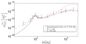
Figure 11: The recombination coefficient for Cs-Cs-Cs, $\alpha_{111}^{(1)}$, at different temperatures plotted with experimental data from Berninger2011 ; Huang2014 . The optical model parameters are $\rho_{cut}=1.4a_{0}$ and $V_{imag}=16\frac{\hbar^{2}}{ma_{0}^{2}}$.

We show the calculated results on fig. 11, where the second Efimov peak is obtained without any adjustments beyond the first peak. The experimental results are not completely commensurable, since the first experiment was done at a temperature of about 15 nK, and the second experiment at 9.6 nK. We can circumvent this by using the fact that temperatures of this value are insignificant at small values of the scattering length. The data for the first peak from the first experiment Berninger2011 can therefore be assumed to arise for the same temperature of 9.6 nK as the second peak in the second experiment Huang2014 . Both temperatures are much smaller than the upper temperature limit estimated to be $1\mu K$ for a realistic calculation.

The absolute value around the first peak and for big $a$ is generally remarkably close to the experimental value. However, the calculated recombination coefficient is much too small at small $a$, where the temperature has no influence. The theoretical results follow the overall $a^{4}$ rule of recombination dependence and these small $a$ deviations must therefore arise from other processes contributing to the experimental values.

The calculated temperature dependence for larger scattering lengths is in very good agreement with the measurements. This is remarkable, since a reduction in temperature to 1 nK results in a fairly dramatic change of the recombination curve at large values of $a$. The consequence is that a moderate temperature of a few nK already smears out the second Efimov peak, and prohibits observation. We then conclude that using the correct temperature gives a shape that is in pretty good agreement with the experimental results. However, the second peak is dislocated compared to the ideal Efimov scaling factor of 22.7, which predicts this peak to be at around $a_{12}=-21800~{}a_{0}$. In the experiment, it is found at approximately $-17000~{}a_{0}$, while the calculation gives the peak at $-15800~{}a_{0}$.

Overall, the results of this comparison with experiments for identical bosons are encouraging. The temperature effects are well accounted for and the shape and location of the second Efimov peak is also in broad agreement with data, for phenomenological parameters fitted to the first peak. Our model seems to work for the well-known mass-balanced case, and comparison to data for mass-imbalanced systems should then be considered.

V.2 The ¹³³Cs-¹³³Cs-⁷Li recombination

The crucial parameter is the scattering length, $a_{12}=a_{\mathrm{L}iCs}$, which has to be very large to provide the Efimov effect. However, in addition also $a_{11}=a_{\mathrm{C}sCs}$ is important for quantitative predictions. The overall $a_{12}^{4}$ scaling is modified for a finite value of $a_{11}$, which is determined by the magnetic field through the Feshbach resonance of the system as described in Eq.(45). It is then interesting to look for effects in the recently obtained two sets of experimental data pires2014 ; tung2014 . They are in broad agreement, although the details are a little different. In tung2014 3 Efimov resonances are reported, where the third one is very hard to distinguish from the background due to finite temperature effects. In pires2014 the recombination coefficient is given as a function of $a_{12}$, which allows an easy comparison with our calculations.

The experimental conditions in pires2014 provide the parameters in Eq.(46) for the interspecies (Cs-Li) Feshbach-resonance of the prepared spin-states, that is

$$a_{bg}=-28.5a_{0}\;,\;\Delta=61.4~{}G\;,\;B_{0}=842.9~{}G\;,$$ (46)

which by insertion in Eq.(45) gives the variation of $a_{12}$. The $a_{11}$ scattering length is estimated to run between $-1200a_{0}\text{ and }-1500a_{0}$ pires2014 , so we have chosen a constant intermediate value of $a_{11}=a_{CsCs}=-1350a_{0}$.

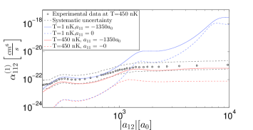
Figure 12: The recombination coefficient for Cs-Cs-Li,$\alpha_{112}^{(1)}$ as a function of the interspecies scattering length, for $a_{11}=0$ and $a_{11}=-1350a_{0}$, plotted with the experimental data from pires2014 . The optical model parameters are $\rho_{cut}=0.258a_{0}$ , $V_{imag}=100\frac{\hbar^{2}}{ma_{0}^{2}}$ for $a_{11}=-1350a_{0}$ and $\rho_{cut}=0.20a_{0}$ , $V_{imag}=240\frac{\hbar^{2}}{ma_{0}^{2}}$ for $a_{11}=0$. One small temperature of 1 nK and the experimental temperature of 450 nK are shown.

We compare theoretical and experimental results in fig. 12 where both temperature and $a_{11}$ dependence are shown. We first note that there is a pretty good correspondence between the experimental data at 450 nK and the theoretical prediction at 450 nK with the suggested finite value of $a_{11}$. The shape is nicely reproduced and the absolute value is within the systematic uncertainty. We emphasize that the calculations for vanishing $a_{11}=0$ does not describe the data quantitatively at 450 nK. The absolute value and the shape is only correct when the enhancement of $\alpha_{112}^{(1)}$ at small values of $a_{12}$, due to finite values of $a_{11}$, is taken into account. We also draw attention to the fact that for a substantial finite value of $|a_{11}|$, $\alpha_{112}^{(1)}$ is no longer independent of energy at small values of $|a_{12}|$. The temperature of 450 nK is not far from $1\mu K$, that is upper temperature limit in a realistic calculation. But the data is described very well.

It seems like the calculated values of $\alpha_{ijk}^{(i)}$ describe the relative behaviour of different recombinations well. The recombination coefficient for Cs-Cs-Li is larger than for Cs-Cs-Cs for both the experimental and the calculated values. The calculated values of both are within experimental uncertainty. The relative location of the Efimov resonances depends on the finite value of $a_{11}$. For the Cs-Cs-Li system the limiting values are 4.8766 or 4.7989, however, which means that we do not expect any noteworthy difference. The 3 Efimov resonances in tung2014 are well suited for testing the theoretical prediction for the Efimov resonances.

We use the value, $B_{0}=942.75$, of the resonant magnetic field. The two reported different values of $B_{0}$ are within the experimental uncertainties of both experiments. In table 3, we compare predicted and experimental values for the Efimov peaks when the optical model parameters are adjusted to reproduce either first ($\rho_{cut}=0.258a_{0}$) or second peak ($\rho_{cut}=0.28a_{0}$).

Table 3: The values of $\Delta B=B-B_{0}$ determined to give the first or second Efimov peak for Cs-Cs-Li, while the other two peaks ( second or first as well as third) are predicted with that set of corresponding optical model parameters.

	1st peak	2nd peak	3rd peak
Experimental value of $\Delta B$ [G]	5.61(16)	1.07(2)	0.22(4)
$\Delta B$ [G] fitted to 2nd peak	5.8	1.07	0.21
$\Delta B$ [G] fitted to 1st peak	5.65	1.03	0.2

Then in both cases the third peak is in agreement with calculations within the experimental uncertainty. However, this does not say much, since a small change in magnetic field results in a huge change in the scattering length, see Eq.(46) and Eq.(45). Due to this, it is also hard to determine an accurate $\rho_{cut}$ value which reproduces the very weak third peak. The two predicted peaks in the two fits are at the edge allowed by the experimental uncertainty, and as such they are still very close to the observed values. The finite temperature effects are also likely to move the locations slightly, which might explain smaller deviation.

We can now calculate the inter-species scattering lengths corresponding to the experimental peak values by using Eq.(46) with $B_{0}=942.75$, which yields $|a^{(-)}_{1}|=331.5a_{0}$, $|a^{(-)}_{2}|=1621a_{0}$ and $|a^{(-)}_{3}|=7777.5a_{0}$. This gives a Efimov scaling of 4.8911 between the first two peaks and 4.7980 between the last two peaks. These values are in agreement with the Efimov scaling found by going to the universal limits of infinite scattering lengths, 4.8766 or 4.7989, depending on whether there is two or three contributing resonant interactions.

V.3 Universal properties of optical parameters

For identical bosons ref.Peder2013 proposes a possible relation between the optical model parameters and the van der Waals length of the system. This is motivated by the recent findings in equal mass systems Berninger2011 of a universal relation between the three-body parameter and the two-body van der Waals length naidon2011 ; chin2011 ; wang2012a ; schmidt2012 ; peder2012 ; naidon2012 ; wang2012b . We can expand this idea to the mass-imbalanced system. The three van der Waals lengths which we will compare with is for Cs-Cs, Li-Li and Cs-Li respectively $202a_{0}$, $65a_{0}$ and $44.8a_{0}$ Pethich2002 ; Dervianko2001 . The crucial parameter is $\rho_{cut}$ which by definition is a hyper-radius. From the definition in Eq.(1) we can analogously define a hyper-radial van der Waals length as

$$\rho_{vdW}^{2}=\frac{2R}{1+2R}\frac{\mu_{11}}{m}r_{vdW,11}^{2}+\frac{1+R}{1/2+R}\frac{\mu_{12}}{m}r_{vdW,12}^{2}\;,$$ (47)

where the distance between particles is replaced by the corresponding two-body van der Waals lengths, and the related two-body reduced masses, $\mu_{11}$ and $\mu_{12}$, are introduced and $R=\frac{m_{1}}{m_{2}}$.

For identical particles with $m$ equal to the mass of the particles, this hyper-radius reduces to the van der Waals length, $\rho_{vdW}^{2}=r_{vdW,11}^{2}$, which in ref.Peder2013 was compared to $\rho_{cut}$ by simple division. For three identical particles we find respectively $\rho_{cut}/\rho_{vdW}=0.0069$ and $\rho_{cut}/\rho_{vdW}=0.0063$ with the parameters for Cs-Cs-Cs and Li-Li-Li.

For the mass-imbalanced system the (identical) interactions between the heavy and the two light particles is as dicussed expected to be the dominating contribution. This means that the last term in Eq.(47) should be the largest while the first term should vanish when the corresponding scattering length, $a_{11}$, between the identical heavy particles is relatively small. Furthermore, when $a_{11}$ is finite and begins to contribute the recombination peak moves. To keep the peak location independent of $a_{11}$ we therefore varied $\rho_{cut}$ slightly with $a_{11}$. This addition to $\rho_{cut}$ has to come from the first term of Eq.(47) which should vary from zero to a given finite contribution when $|a_{11}|=\infty$. Thus we can parametrize by

$$\rho_{vdW}^{2} = \frac{2R}{1+2R}\frac{\mu_{11}}{m}\frac{|a_{11}|}{(f_{11}a_{0}+|a_{11}|R^{2}f(R))}r_{vdW,11}^{2}$$ (48)

$$+ \frac{1+R}{1/2+R}\frac{\mu_{12}}{m}r_{vdW,12}^{2}\;,$$

where we suggest to use $f_{11}=10^{7}$. For equal masses and $a_{11}\rightarrow\infty$ this reduces to Eq.47 for equal masses. For unequal masses the $R^{2}$ factor ensures that for $a_{11}\rightarrow\infty$, the term still doesn’t become dominant, in correspondence with the moderate change in $\rho_{cut}$, even as big values of $|a_{11}|$ were used numerically. We use $f(R)=1$, but perhaps a more complicated function is required. For the experimental value, $a_{11}=-1350a_{0}$ ($\rho_{cut}=0.258a_{0}$), we then get $\rho_{cut}/\rho_{vdW}=0.0057$ close to the experimental values for identical particles.

The strength, $V_{imag}$, can also be compared to the natural unit for a van der Waals interaction, $V_{vdW}=\hbar^{2}/m\rho_{rdW}^{2}$. which amounts to $V_{imag}/V_{vdW}=6.53\cdot 10^{5},2.87\cdot 10^{5},2.03\cdot 10^{5}$ for Cs-Cs-Cs, Li-Li-Li, and Cs-Cs-Li, respectively. The value of $\frac{m}{\hbar}V_{imag}\rho_{cut}^{2}$ is constant for a given location and shape in a specific system. The numerical values from our calculation are for this quantity 31.3600, 11.4308, 6.6564 for the systems Cs-Cs-Cs, Li-Li-Li and Cs-Cs-Li.

The upshot of these comparisons is that a possible approximate value of $\rho_{cut}$ for a system can be obtained by $\rho_{cut}\approx 0.006\rho_{vdW}$. In addition the value of $V_{imag}$ to within a factor of two seems obtainable by $V_{imag}\approx 3\cdot 10^{5}V_{vdW}$. Finally the value $\frac{m}{\hbar}V_{imag}\rho_{cut}^{2}$ in different systems are within the same order of magnitude.

VI Discussion and Outlook

We have developed a method for calculating the three-body recombination coefficient of mass-imbalanced three-body systems at negative values of the scattering lengths and for small energies. In order to do this we employed the hyper-spherical method, zero-range potentials and the Faddev decomposition to calculate the lowest-order adiabatic potential.

In addition we formulated and explored the optical model to calculate recombination processes into deep dimers. This method introduces two phenomenological optical parameters, strength and range, which respectively determine location and shape of the Efimov resonances. We then developed two methods for finding the recombination coefficients of both mass-balanced and mass-imbalanced systems. By means of the traditional S-matrix method and by a new method, where the decay rate of bound states in a box due to the presence of the optical potential is calculated. In general the results obtained with the two methods are essentially indistinguishable, although differing in numerical inaccuracies. As they tend to complement each other, we choose the most convenient method in actual calculations.

The model was tested against the experimental data on recombination coefficients in Cs-Cs-Cs and Cs-Cs-Li systems as functions of the Feshbach tuned scattering lengths. In both cases, after fitting the range and the strength of the imaginary potential to the first peak, the model was able to describe quantitatively the whole curve including the temperature effects.

The two-parameter fits of strength and hyper-radius of the imaginary part of the optical potential are very efficient for both position and shape of the recombination peaks. It is also remarkable that the absolute values of the experimental recombination coefficients are reproduced within the experimental uncertainty.

Using the developed methods we have reached a number of conclusions. The main conclusions are that recombination is dominated by the heavy-heavy-light process and mainly determined by the heavy-light scattering length. But the heavy-heavy scattering length is important for obtaining the correct value of the recombination coefficients, as it enhances the recombination probability and modifies the behaviour as a function of the heavy-light scattering length. For a large mass ratio the Efimov scaling is determined entirely by the heavy-light scattering length, but for a smaller mass ratio finite values of the heavy-heavy scattering length becomes important. The Efimov scaling then moves continuously between values from two and three resonating subsystems.

The focus of this paper has been the case where all scattering lengths are negative, but it could be just as relevant to investigate two negative, one positive or two positive, one negative scattering length cases. Since a finite value of the heavy-heavy scattering length can substantially alter the absolute value of a given two-component recombination, it may be interesting to test the three-body recombination for the same system at different Feshbach resonances experimentally, in order to further confirm this prediction.

For small mass-ratios we find a big difference in the Efimov scaling between peaks as the heavy-heavy scattering length is increased. It may be fruitful to investigate the intermediate area between two and three resonant subsystems in more theoretical detail. In addition a Feshbach resonance in a two-component gas with small mass-ratio, in which the heavy-heavy scattering length is big in the same area as the inter-species scattering length would allow investigation of this effect.

The authors thank PK Sørensen for invaluable help on the numerical details. The authors are grateful for enlightening discussions with A. G. Volosniev, N. Winter, N. B. Jørgensen, L. J. Wacker, J. F. Sherson and J. J. Arlt. This reserach was supported by the Danish Council for Independent Research DFF Natural Sciences.

References

- (1) Ottenstein T B, Lompe T, Kohnen M,Wenz A N and Jochim S 2008 Phys.Rev.Lett. 101, 203202.
- (2) Pollack S E, Dries D, and Hulet R G 2009, Science 326, 1683.
- (3) Zaccanti M et al. Nat. Phys. 5, 586.
- (4) Gross N, Shotan Z, Kokkelmans S and Khaykovich L 2009 Phys. Rev. Lett. 103, 163202-.
- (5) Huckans J H, Williams J R, Hazlett E L, Stites R W and O’Hara K M 2009 Phys.Rev.Lett. 102, 165302.
- (6) Williams J R, Hazlett E L, Huckans J H, Stites R W, Zhang Y and O’Hara k M 2009 Phys.Rev.Lett. 103, 130404.
- (7) Lompe T, Ottenstein T B, Serwane F, Wenz A N, Zürn G and Jochim S 2010 Science 330, 9405.
- (8) Gross N, Shotan Z, Kokkelmans S and Khaykovich L 2010 Phys. Rev. Lett. 105, 103203.
- (9) Lompe T, Ottenstein T B, Serwane F, Viering K, Wenz A N, Zürn G and Jochim S 2010 Phys.Rev.Lett. 105, 103201.
- (10) Nakajima S, Horikoshi M, Mukaiyama T, Naidon P and Ueda M 2010 Phys. Rev. Lett. 105, 023201.
- (11) Nakajima S, Horikoshi M, Mukaiyama T, Naidon P and Ueda M 2011 Phys. Rev. Lett. 106, 143201.
- (12) Wild R J, Makotyn P, Pino J M, Cornell E A and Jin D S 2012 Phys. Rev. Lett. 108, 145305.
- (13) Machtey O, Kessler D A and Khaykovich L 2012 Phys. Rev. Lett. 108, 130403.
- (14) Machtey O, Shotan Z, Gross N and Khaykovich L 2012 Phys. Rev.Lett. 108, 210406.
- (15) Knoop S, Borbely J S, Vassen W, Kokkelmans S J J M F 2012 Phys. Rev. A 86, 062705.
- (16) Rem B S et al. 2013 Phys.Rev.Lett. 110 , 163202.
- (17) Dyke P, Pollack S E, Hulet R G 2013 Phys. Rev. A 88 023625.
- (18) Berninger M et al. 2011 Phys. Rev. Lett. 107 120401.
- (19) Huang B, Sidorenkov L A, Grimm R and Hutson J M 2014 Phys. Rev. Lett. 112 190401.
- (20) Pires R, Ulmanis J, Häfner S, Repp M, Arias A, Kuhnle E D and Weidemüller M 2014 Phys. Rev. Lett. 112 250404.
- (21) Tung S-K, Jimenez-G K, Johansen J, Parker C-V and Chin C 2014 Phys. Rev. Lett. 113 240402.
- (22) Pires R, Ulmanis J, Häfner S, Pires R, Kuhnle E D, Weidemüller M and Tiemann E 2015 arXiv:1501.04799
- (23) Zinner N T and Nygaard N G 2014 arXiv:1403.0759
- (24) Helfrich K, Hammer H W and Petrov D S Phys. Rev. A 81, 042715.
- (25) Fedorov D V and Jensen A S 2003 Europhys. Lett. 62, 336.
- (26) Braaten E, Hammer H W 2006 Phys. Rep. 428 259.
- (27) Nielsen E, Fedorov D V, Jensen A S and Garrido E 2001 Phys. Rep. 347 373.
- (28) Fedorov D V and Jensen A S 2001 J. Phys. A: Math. Gen. Phys. 34, 6003.
- (29) Nielsen E, Fedorov D V and Jensen A S 1998 J. Phys. B: At. Mol. Opt. Phys. 31 4085.
- (30) Siemens P J and Jensen A S, Elements of Nuclei, Lecture notes and supplements in Physics, Addison-Wesley Publishing Company 1987, pp 48-54.
- (31) Sørensen P K, Fedorov D V, Jensen A S and Zinner N T 2013 Phys. Rev. A 88 042518.
- (32) Roy S et al. 2013 Phys. Rev.Lett. 111, 053202
- (33) Mehta N P, Rittenhouse S T, D’Incao J P, Stecher J, and Greene C H Phys. Rev. Lett. 103, 153201.
- (34) Kagan Y,Svistunov B V and Shlyapnikov G V 1985 JETP Lett. 42, 209
- (35) Garrido E, Kievsky A, and Viviani M 2014 Phys. Rev.C 90, 014607
- (36) Abramowitz and Stegun, Handbook of Mathematical Functions with Formulas, Graphs, and Mathematical Tables, Dover Publications 1972 pp 364
- (37) Nielsen E and Macek J H 1999 Phys. Rev. Lett. 83 1566.
- (38) Esry B D, Greene C H and Burke J P 1999 Phys. Rev. Lett. 83, 1751
- (39) Sørensen P K, Fedorov D V, Jensen A S and Zinner N T 2013 J. Phys B: At. Mol. Opt. Phys. 46 075301.
- (40) Sørensen P K, Three-Body Recombination in Cold Atomic Gases, PhD thesis, Aarhus University 2013
- (41) Naidon P, Hiyama E and Ueda M 2012 Phys. Rev. A 86 012502
- (42) Chin C 2011 arXiv:1111.1484v2.
- (43) Wang J, D’Incao J P, Esry B D and Greene C H 2012 Phys. Rev. Lett. 108 263001
- (44) Schmidt R, Nath S P and Zwerger W 2012 Eur. Phys. J. B 85 386
- (45) Sørensen P K, Fedorov D V, Jensen A S and Zinner N T 2012 Phys. Rev. A 86 052516
- (46) Naidon P, Endo S and Ueda M 2014 Phys. Rev. Lett. 112 105301
- (47) Wang Y, Wang J, D’Incao J P and Greene C H 2012 Phys. Rev. Lett. 109 243201
- (48) Pethick C J and Smith H, Bose-einstein condensation in dilute gases. Cambridge, 2002
- (49) Derevianko A, Babb J F and Dalgarno A 2001 Phys. Rev. A 63 052704