Dependence and phase changes in random $m$-ary search trees

Abstract

We study the joint asymptotic behavior of the space requirement and the total path length (either summing over all root-key distances or over all root-node distances) in random $m$-ary search trees. The covariance turns out to exhibit a change of asymptotic behavior: it is essentially linear when $3\leqslant m\leqslant 13$ but becomes of higher order when $m\geqslant 14$. Surprisingly, the corresponding asymptotic correlation coefficient tends to zero when $3\leqslant m\leqslant 26$ but is periodically oscillating for larger $m$, and we also prove asymptotic independence when $3\leqslant m\leqslant 26$. Such a less anticipated phenomenon is not exceptional and we extend the results in two directions: one for more general shape parameters, and the other for other classes of random log-trees such as fringe-balanced binary search trees and quadtrees. The methods of proof combine asymptotic transfer for the underlying recurrence relations with the contraction method.

AMS 2010 subject classifications. Primary 60F05, 68Q25; secondary 68P05, 60C05, 05A16.

Key words. $m$-ary search tree, correlation, dependence, recurrence relations, fringe-balanced binary search tree, quadtree, asymptotic analysis, limit law, asymptotic transfer, contraction method.

1 Introduction

The $m$-ary search trees are a class of data structures introduced by Muntz and Uzgalis [35] in 1971 in computer algorithms to support efficient searching and sorting of data; see the next section for more details. When constructed from a random permutation of $n$ elements, the space requirement (total number of nodes to store the input) $S_{n}$ of such random $m$-ary search trees ($m\geqslant 3$) is known to exhibit a phase change phenomenon: its distribution is asymptotically Gaussian for large $n$ when the branching factor $m$ satisfies $3\leqslant m\leqslant 26$ but does not approach a limit law when $m\geqslant 27$; see [8, 22, 30, 31] and the references therein. On the other hand, it is also known that the total key path length $K_{n}$ (the sum over all distances from the root to any key) does not change its limiting behavior when $m$ varies, and tends asymptotically, after properly centered and normalized, to a limit law for each $m\geqslant 3$. Another closely related shape measure, the total node path length $N_{n}$ (summing over all distances from the root to any node) also follows asymptotically a very similar behavior.

Our motivating question was “how does $K_{n}$ or $N_{n}$ depend on $S_{n}$?” Surprisingly, despite the strong dependence of the definition of $N_{n}$ on $S_{n}$ (see (2)), we show that the correlation coefficient $\rho(S_{n},N_{n})$ satisfies

$$\rho(S_{n},N_{n})\sim\begin{cases}0,&\text{if}\ 3\leqslant m\leqslant 26;\\ \displaystyle F_{\rho}(\beta\log n),&\text{if}\ m\geqslant 27,\end{cases}$$ (1)

where $F_{\rho}(t)$ is a $2\pi$-periodic function and $\beta=\beta_{m}$ is a structural constant depending on $m$. The same type of results also holds for $\rho(S_{n},K_{n})$. In words, $N_{n}$ and $S_{n}$ are asymptotically uncorrelated for $3\leqslant m\leqslant 26$ and their correlation fluctuates (between $-1$ and $1$) for $m\geqslant 27$; see Figure 1 for an illustration.

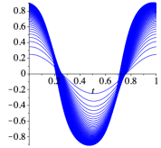
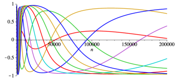
Figure 1: The periodic functions $F_{\rho}(2\pi t)$ for $m=27,\dots,100$ (left) and $F_{\rho}(\beta\log n)$ for $m=27,54,\dots,270$ (right).

One reason why the above result (1) may seem less or even counter-intuitive is because of the seemingly strong dependence of $N_{n}$ on $S_{n}$ in the recursive equations satisfied by both random variables

$$\begin{cases}S_{n}\stackrel{{\scriptstyle d}}{{=}}S_{I_{1}}^{(1)}+\cdots+S_{I_{m}}^{(m)}+1,\\ N_{n}\stackrel{{\scriptstyle d}}{{=}}N_{I_{1}}^{(1)}+\cdots+N_{I_{m}}^{(m)}+S_{I_{1}}^{(1)}+\cdots+S_{I_{m}}^{(m)},\end{cases}$$ (2)

where the $(S_{i}^{(r)},N_{i}^{(r)})$’s are independent copies of $(S_{i},N_{i})$, respectively, also independent of $(I_{1},\ldots,I_{m})$, and

$${\mathbb{P}}(I_{1}=i_{1},\dots,I_{m}=i_{m})=\frac{1}{\binom{n}{m-1}},$$ (3)

when $i_{1},\dots,i_{m}\geqslant 0$ and $i_{1}+\cdots+i_{m}=n-m+1$. Intuitively, we expect, from the above relations, that the node path length $N_{n}$ would have a strong correlation with $S_{n}$.

While one might ascribe this seemingly less intuitive result to the possibly nonlinear dependence between $N_{n}$ and $S_{n}$, we enhance such an uncorrelation by a stronger joint limit law for $(S_{n},N_{n})$ for $3\leqslant m\leqslant 26$, which further accents the asymptotic independence between $N_{n}$ and $S_{n}$; for $m\geqslant 27$, they are asymptotically dependent and we will derive a precise characterization of their joint asymptotic distributions. See Section 4 for a more precise description of the joint asymptotic behaviors of $(S_{n},N_{n})$ and $(S_{n},K_{n})$.

Let $\alpha$ denote the real part of the second largest zero (in real parts) of the indicial equation $\Lambda(z)=0$, where

$$\Lambda(z)=z(z+1)\cdots(z+m-2)-m!.$$ (4)

Then $\alpha<1$ for $m<14$ and $1<\alpha<\frac{3}{2}$ for $14\leqslant m\leqslant 26$; see Table 1. Also $\alpha\to 2$ as $m\to\infty$; see [30, Sec. 3.3] for more properties of $\alpha$.

$m$	$3$	$4$	$5$	$6$	$7$	$8$	$9$	$10$
$\alpha$	$-3$	$-2.5$	$-1.5$	$-0.768$	$-0.260$	$0.101$	$0.366$	$0.568$
$m$	$11$	$12$	$13$	$14$	$15$	$16$	$17$	$18$
$\alpha$	$0.726$	$0.852$	$0.955$	$1.040$	$1.112$	$1.173$	$1.226$	$1.272$
$m$	$19$	$20$	$21$	$22$	$23$	$24$	$25$	$26$
$\alpha$	$1.313$	$1.348$	$1.380$	$1.409$	$1.435$	$1.458$	$1.479$	$1.499$

Table 1: Approximate numerical values of $\alpha=\alpha_{m}$ for $3\leqslant m\leqslant 26$.

The main reason that $\rho(S_{n},N_{n})\to 0$ for $3\leqslant m\leqslant 26$ is roughly that their covariance is of order $\max\{n\log n,n^{\alpha}\}$ (see Theorem 2.3 below), while the standard deviations for $S_{n}$ and $N_{n}$ are of orders $\sqrt{n}$ and $n$, respectively. So that

$$\rho(S_{n},N_{n})=\begin{cases}O\left(n^{-\frac{1}{2}}\log n\right),&\text{if }3\leqslant m\leqslant 13;\\ O\left(n^{-\frac{3}{2}+\alpha}\right),&\text{if }14\leqslant m\leqslant 26,\end{cases}$$

which tends to zero in both cases. Briefly, the large quadratic variance of $N_{n}$ is the major cause of the asymptotic independence between $S_{n}$ and $N_{n}$ for $3\leqslant m\leqslant 26$.

Such a change from being asymptotically independent to being asymptotically dependent under a varying structural parameter is not an exception. We will extend our study to fringe-balanced binary search trees and quadtrees; a typical related instance states that: the number of comparisons (or exchanges) used by the median-of-$(2t+1)$ quicksort is asymptotically independent of the number of partitioning stages when $0\leqslant t\leqslant 58$, but is asymptotically dependent for $t\geqslant 59$.

2 $M$-ary search trees

We briefly introduce $m$-ary search trees in this section and then describe the random variables we are studying in this paper.

Figure 2: Three $m$-ary search trees for the sequence $\{6,2,4,8,7,1,5,3,10,9\}$: $m=2$ (left), $m=3$ (middle), and $m=4$ (right).

An $m$-ary tree is either empty or comprises of a single node called the root, together with an ordered $m$-tuple of subtrees, each of which is, by definition, an $m$-ary tree. Given a sequence of numbers, say $\{x_{1},\dots,x_{n}\}$, we construct an $m$-ary search tree by the following procedure, $m\geqslant 2$. If $1\leqslant n<m$, then all keys are stored in the root. If $n\geqslant m$ the first $m-1$ keys are sorted and stored in the root, the remaining keys are directed to the $m$ subtrees, each corresponding to one of the $m$ intervals formed by the $m-1$ sorted keys in the root node; see Figure 2 for an illustration (the rectangular nodes denote yet empty subtrees of full nodes). If the $m-1$ numbers in the root are $x_{j_{1}}<\cdots<x_{j_{m-1}}$, then the keys directed to the $i$th subtree all have their values lying between $x_{j_{i-1}}$ and $x_{j_{i}}$, where $x_{j_{0}}:=0$ and $x_{j_{m}}:=n+1$. All subtrees are themselves $m$-ary search trees by definition. For more details, see Mahmoud [30].

While the practical usefulness of $m$-ary search trees is largely overshadowed by their balanced counterparts such as $B$-trees, they have been a source of many interesting phenomena, which are to some extent universal. The study of $m$-ary search trees is thus of fundamental and prototypical value. Furthermore, the close connection between $m$-ary search trees and generalized quicksort adds an extra dimension to the richness of diverse variations and their asymptotic behaviors.

2.1 Space requirement and total path lengths

Assume that the input sequence $\{x_{1},\dots,x_{n}\}$ is a random permutation, where all $n!$ permutations are equally likely. The resulting $m$-ary search tree constructed from the given sequence is then called a random $m$-ary search tree. The major shape parameters of particular algorithmic interest include the depth, the height, the space requirement, the total path length, and the profile; see [11, 30] for more information. We are concerned in this paper with the following three random variables.

• $S_{n}$ (space requirement): the total number of nodes used to store the input; the three trees in Figure 2 have $S_{10}$ equal to $10,6,6$, respectively. If $m=2$, then $S_{n}\equiv n$; if $m\geqslant 3$, we can compute $S_{n}$ recursively by $S_{0}=0$, and

  $$S_{n}\stackrel{{\scriptstyle d}}{{=}}\begin{cases}1,&\text{if }1\leqslant n<m,\\ S_{I_{1}}^{(1)}+\cdots+S_{I_{m}}^{(m)}+1,&\text{if }n\geqslant m,\end{cases}$$ (5)

  where the $S_{i}^{(r)}$’s are independent copies of $S_{i}$, $1\leqslant r\leqslant m$, $0\leqslant i\leqslant n-m+1$, and independent of $(I_{1},\ldots,I_{m})$ defined in (3).

• $K_{n}$ (key path length, KPL): the sum of the distance between the root and each key; for the trees in Figure 2, $K_{10}=\{19,11,8\}$, respectively. For $m\geqslant 2$, $K_{n}$ satisfies the recurrence

  $$K_{n}\stackrel{{\scriptstyle d}}{{=}}\begin{cases}0,&\text{if }n<m,\\ K_{I_{1}}^{(1)}+\cdots+K_{I_{m}}^{(m)}+n-m+1,&\text{if }n\geqslant m,\end{cases}$$ (6)

  where the $K_{i}^{(r)}$’s are independent copies of $K_{i}$, $1\leqslant r\leqslant m,0\leqslant i\leqslant n-m+1$, independent of $(I_{1},\ldots,I_{m})$.

• $N_{n}$ (node path length, NPL): the sum of the distance between the root and each node; so that $N_{10}=\{19,7,6\}$ for the three trees in Figure 2. Obviously, $N_{n}=K_{n}$ when $m=2$. When $m\geqslant 3$,

  $$N_{n}\stackrel{{\scriptstyle d}}{{=}}\begin{cases}0,&\text{if }n<m,\\ N_{I_{1}}^{(1)}+\cdots+N_{I_{m}}^{(m)}+S_{I_{1}}^{(1)}+\cdots+S_{I_{m}}^{(m)},&\text{if }n\geqslant m,\end{cases}$$ (7)

  where the $(N_{i}^{(r)},S_{i}^{(r)})$’s are independent copies of $(N_{i},S_{i})$, $1\leqslant r\leqslant m,0\leqslant i\leqslant n-m+1$, independent of $(I_{1},\ldots,I_{m})$.

While the first two random variables have been widely studied in the literature, NPL was only considered previously in [4, 21] in connection with the process of cutting trees. In addition to this, our interest was to understand the extent to which the asymptotic independence for small $m$ between $S_{n}$ and $K_{n}$ subsists when the “toll function” changes from a linear function to a function that is random and may depend on $S_{n}$.

2.2 A summary of known results

Let $H_{m}:=\sum_{1\leqslant j\leqslant m}j^{-1}$. Knuth [27, §6.2.4] was the first to show that

$$\mathbb{E}(S_{n})\sim\phi n,\quad\text{where}\quad\phi:=\frac{1}{2(H_{m}-1)},$$

(see also [1]). Here $\phi$ denotes the “occupancy constant”, which will appear all over our analysis. Mahmoud and Pittel [31] improved the result and derived an identity for $\mathbb{E}(S_{n})$, which implies in particular that

$$\mathbb{E}(S_{n})=\phi(n+1)-\frac{1}{m-1}+O\left(n^{\alpha-1}\right),$$

where $\alpha$ has the same meaning as in Introduction; see (4). They also discovered and proved the surprising result for the variance

$$\mathbb{V}(S_{n})\sim\begin{cases}C_{S}n,&\text{if }3\leqslant m\leqslant 26;\\ F_{1}(\beta\log n)n^{2\alpha-2},&\text{if }m\geqslant 27,\end{cases}$$

where $C_{S}$ is a constant depending on $m$, $F_{1}$ is a $\pi$-periodic function given in (28), $\alpha+i\beta$ is the second largest zero (in real part) with $\beta>0$ of the equation $\Lambda(z)=0$ (see (4)), and $2\alpha-2>1$ for $m\geqslant 27$. See also [9, 25, 33] for a closely related fragmentation model with the same asymptotic behavior. A central limit theorem for $S_{n}$ was then proved for $3\leqslant m\leqslant 26$ in [28, 31]; see also [30] for more details. Their approach is based on an inductive approximation argument.

By the method of moments, two authors of this paper re-proved in [8] the central limit theorem for $S_{n}$ when $3\leqslant m\leqslant 26$; the same approach was also used to establish the nonexistence of a limit law for $S_{n}$ due to inherent oscillations. Moreover, the convergence rates to the normal distribution were characterized in [22] by a refined method of moments, which undergo further change of behaviors.

Then several different approaches were developed in the literature for a deeper understanding of the “phase change” at $m=26$; these include martingale [6], renewal theory [25], urn models [23, 32], contraction method [13, 39], method of moments [22], statistical physics [9, 33], etc.

On the other hand, the KPL for general $m\geqslant 2$ was first studied by Mahmoud [29] and he proved

$$\mathbb{E}(K_{n})=2\phi n\log n+c_{1}n+o(n),$$

for some explicitly computable constant $c_{1}$; see (25). The variance was computed in [30, §3.5] and satisfies ($H_{m}^{(2)}:=\sum_{1\leqslant j\leqslant m}j^{-2}$)

$$\mathbb{V}(K_{n})\sim C_{K}n^{2},\quad\text{where}\quad C_{K}=4\phi^{2}\left(\tfrac{(m+1)H_{m}^{(2)}-2}{m-1}-\tfrac{\pi^{2}}{6}\right).$$ (8)

The corresponding limit law was characterized in [38] by the contraction method

$$\frac{K_{n}-\mathbb{E}(K_{n})}{n}\stackrel{{\scriptstyle d}}{{\longrightarrow}}K,$$ (9)

where $K$ is given by the recursive distributional equation (75); see also [4, 34] for a general framework.

For NPL $N_{n}$, Broutin and Holmgren [4] proved that

$$\mathbb{E}(N_{n})=2\phi^{2}n\log n+c_{2}n+o(n),$$

for some constant $c_{2}$ (for which no numerical value was provided); a series expression of $c_{2}$ is given in [21, p. 156]. We will give an alternative proof of this result below with tools from [8, 14]. Our approach makes the computation of $c_{2}$ feasible (although its exact value is not needed); see (31).

It should be mentioned that there is a large literature on $K_{n}$ when $m=2$ because it is identical to the comparison cost used by quicksort. Many fine results were obtained; see, for example, the recent papers [3, 12, 17, 20, 37, 41] and the references therein for more information.

2.3 Covariance, correlation, dependence and phase changes

We state in this section our results for the covariance and correlation between the space requirement and the total path lengths (KPL and NPL). The proofs and the tools needed will be given in the next sections.

Unlike the space requirement $S_{n}$ whose variance changes its asymptotic behavior for $m\geqslant 27$, the covariance $\mathrm{Cov}(S_{n},K_{n})$ changes its asymptotic behavior at $m=14$.

Theorem 2.1.

The covariance between $S_{n}$ and $K_{n}$ satisfies

$$\mathrm{Cov}(S_{n},K_{n})\sim\begin{cases}C_{R}n,&\text{if}\ 3\leqslant m\leqslant 13;\\ F_{2}\left(\beta\log n\right)n^{\alpha},&\text{if}\ m\geqslant 14;\end{cases}$$

where $C_{R}$ is a suitable constant and $F_{2}(z)$ is a $2\pi$-periodic function given in (29) below.

This result has the following consequence.

Corollary 2.2.

The correlation coefficient between $S_{n}$ and $K_{n}$ satisfies

$$\rho(S_{n},K_{n})\begin{cases}\rightarrow 0,&\text{if }3\leqslant m\leqslant 26;\\ \sim\displaystyle\frac{F_{2}\left(\beta\log n\right)}{\sqrt{C_{K}F_{1}(\beta\log n)}},&\text{if }m\geqslant 27,\end{cases}$$

where $C_{K}>0$ is given in (8).

See Figure 1 for two different plots for the periodic functions when $m\geqslant 27$.

The same consideration extends easily to clarify the correlation between space requirement and NPL.

Theorem 2.3.

The covariance between $S_{n}$ and $N_{n}$ satisfies

$$\mathrm{Cov}(S_{n},N_{n})\sim\begin{cases}2\phi C_{S}n\log n,&\text{if}\ 3\leqslant m\leqslant 13;\\ \phi F_{2}\left(\beta\log n\right)n^{\alpha},&\text{if}\ m\geqslant 14,\end{cases}$$

where $C_{S}$ is as in Section 2.2. Moreover, the variance of $N_{n}$ satisfies

$$\mathbb{V}(N_{n})\sim\phi^{2}C_{K}n^{2}.$$

Notice the appearance of an extra $\log n$ factor when $3\leqslant m\leqslant 13$, which reflects the additional random effect introduced by the toll function in (7). These estimates imply the following consequence.

Corollary 2.4.

The correlation coefficient $\rho(S_{n},N_{n})$ satisfies

$$\rho(S_{n},N_{n})\begin{cases}\rightarrow 0,&\text{if }3\leqslant m\leqslant 26;\\ \sim\rho(S_{n},K_{n})\sim\displaystyle\frac{F_{2}\left(\beta\log n\right)}{\sqrt{C_{K}F_{1}(\beta\log n)}},&\text{if }m\geqslant 27.\end{cases}$$

The last relation suggests considering the correlation between $K_{n}$ and $N_{n}$.

Corollary 2.5.

The random variable $K_{n}$ is asymptotically linearly correlated to $N_{n}$

$$\rho(K_{n},N_{n})\to 1.$$

Indeed, we will show that

$$\|N_{n}-\phi K_{n}-({\mathbb{E}}(N_{n}-\phi K_{n}))\|_{2}=o(n)$$

which then by Slutsky’s theorem implies that

$$\left(\frac{K_{n}-{\mathbb{E}}(K_{n})}{n},\frac{N_{n}-\mathbb{E}(N_{n})}{n}\right)\stackrel{{\scriptstyle d}}{{\longrightarrow}}(K,\phi K);$$

see (9), Section 4.3 and 4.4.

These results will be proved by working out the asymptotics of the corresponding recurrence relations, which all have the same form

$$a_{n}=m\sum_{0\leqslant j\leqslant n-m+1}\pi_{n,j}a_{j}+b_{n},\qquad(n\geqslant m-1),$$

where

$$\pi_{n,j}=\frac{\binom{n-1-j}{m-2}}{\binom{n}{m-1}}\qquad(0\leqslant j\leqslant n-m+1)$$

is a probability distribution, and $\{b_{n}\}$ is a given sequence (referred to as the toll-function). For that asymptotic purpose, our key tools will rely on the asymptotic transfer techniques (see [8, 14]), which provide a direct asymptotic translation from the asymptotic behaviors of $b_{n}$ to those of $a_{n}$. The remaining analysis will then consist of simplifying some multiple Dirichlet’s integrals.

Since Pearson’s product-moment correlation coefficient $\rho$ is known to be poor in measuring nonlinear dependence between two random variables, we go further by considering the joint limit laws for $(S_{n},K_{n})$ and $(S_{n},N_{n})$, which exhibit a change of behavior depending on whether $3\leqslant m\leqslant 26$ (convergent case) or $m\geqslant 27$ (periodic case): they are asymptotically independent in the former case but dependent in the latter.

Theorem 2.6.

Assume $3\leqslant m\leqslant 26$. Let $(X_{n})_{n}\in\{(K_{n})_{n},(N_{n})_{n}\}$ and $Q_{n}=(X_{n},S_{n})$ denote the vector of KPL or NPL and the space requirement used by a random $m$-ary search tree. Then the convergence in distribution holds:

$$\mathrm{Cov}(Q_{n})^{-1/2}(Q_{n}-\mathbb{E}[Q_{n}])\stackrel{{\scriptstyle d}}{{\longrightarrow}}(X,\mathscr{N}),$$ (10)

where $\mathscr{N}$ has the standard normal distribution and the limit law $(X,\mathscr{N})$ is described in Lemma 4.2; moreover, $X$ and $\mathscr{N}$ are independent.

Theorem 2.7.

Assume $m\geqslant 27$. Let $(X_{n})_{n}\in\{(K_{n})_{n},(N_{n})_{n}\}$ and

$$Y_{n}:=\left(\frac{X_{n}-\mathbb{E}[X_{n}]}{\iota_{X}n},\frac{S_{n}-\phi n}{n^{\alpha-1}}\right)$$

with $\iota_{X}=1$ for $(X_{n})_{n}=(N_{n})_{n}$ and $\iota_{X}=\phi^{-1}$ for $(X_{n})_{n}=(K_{n})_{n}$. Then we have

$$\ell_{2}(Y_{n},(X,\Re(n^{i\beta}\Lambda)))\to 0,$$

where $\beta$ is as in Section 2.2 and $(X,\Lambda)$ is a random vector whose distribution is specified as the unique fixed point solution appearing in Lemma 4.1 for the choice $\gamma=(0,\theta)$ ($\theta$ being defined below in (32)).

See Section 4 for a more precise formulation. The proof is based on the contraction method (see [36]) where we use the above moment asymptotics as input and combine well-known estimates within the minimal $L_{2}$-metric for the convergent case (as in [40]), and those with estimates for the periodic case (as in [13]). Similar proof techniques related to periodic distributional behaviors are also applied in [25, Theorem 1.3(iii)] and [26, Theorem 6.10]. If one is only interested in the asymptotic (univariate) distribution of the NPL $N_{n}$ (the case of the KPL being known before), there are more direct proofs which we also discuss in Sections 4.3 and 4.4.

Our study of the dependence of random variables on random $m$-ary search trees can be extended in at least two directions by the same methods used in this paper, namely, asymptotic transfer techniques and the contraction method.

• Extension to more general linear and $n\log n$ shape measures: That the asymptotic covariance undergoes a phase change after $m=13$ and the asymptotic correlation undergoes a phase change after $m=26$ is not restricted to the space requirement and KPL or NPL. Indeed, we can replace the space requirement by many other linear shape measures such as the number of leaves, the number of nodes of a specified type, the number of occurrences of a fixed pattern, etc. (see [8] for more examples), and KPL or NPL by other shape measures with mean of order $n\log n$ such as summing over the root-node or root-key distance for certain specified nodes or patterns and weighted path length.

• Extension to other random trees of logarithmic height: the same change of asymptotic behaviors from being independent to being dependent under a varying structural parameter also occurs in other classes of random log-trees; we content ourselves with the brief discussion of two classes of random trees: fringe-balanced binary search trees and quadtrees. The behaviors will be however very different for the classes of trees where the underlying distribution of the subtree sizes are dictated by a binomial distribution, which will be examined elsewhere; see a companion paper [18] for more information.

This paper is organized as follows. We prove in the next section our results for the covariances and the correlations. These results are then used to study the bivariate distributional asymptotics in Section 4 by the multivariate contraction method (see [36]). Finally, in Section 5, we discuss the dependence and phase changes in fringe-balanced binary search trees and in quadtrees, where for the former, we study the joint behavior of the size and total path length, while for the latter (since the size is a constant) we consider the joint behavior of the number of leaves and total path length. Also we include a brief discussion for extending the study and results to other shape parameters in Section 5.

3 Correlation between space requirement and path lengths

We prove in this section Theorems 2.1 and 2.3 for the covariances $\text{Cov}(S_{n},K_{n})$ and $\text{Cov}(S_{n},N_{n})$, respectively.

3.1 Preliminaries and recurrences

We collect here the notations to be used in the proofs. Let $m\geqslant 2$ be a fixed integer. For $n\geqslant m$, denote by $I^{(n)}=(I^{(n)}_{1},\ldots,I^{(n)}_{m})$ the vector of the number of keys inserted in the $m$ ordered subtrees of the root in a random $m$-ary search tree with $n$ keys. When the dependence on $n$ is obvious, we write simply $(I_{1},\ldots,I_{m})$. Generate independently $n$ uniform random variables $U_{1},\ldots,U_{n}$ on $[0,1]$. Store the first $m-1$ elements $U_{1},\ldots,U_{m-1}$ in the root-node of the tree. Then they decompose the unit interval $[0,1]$ into spacings of lengths $V_{1},\ldots,V_{m}$, where $V_{j}=U_{(j)}-U_{(j-1)}$ for $j=1,\ldots,m$ with $U_{(0)}:=0,U_{(m)}:=1$ and $U_{(j)}$ for $j=1,\ldots,m-1$ are the order statistics of $U_{1},\ldots,U_{m-1}$. The uniform permutation model implies, that, conditional on $U_{1},\ldots,U_{m-1}$, the vector $I^{(n)}$ has the multinomial distribution with success probabilities $V_{1},\ldots,V_{m}$, namely, we have

$$(I_{1},\ldots,I_{m})\stackrel{{\scriptstyle\mathrm{d}}}{{=}}M(n-m+1;V_{1},\ldots,V_{m}).$$

In particular, we have the convergence

$$\frac{I_{r}}{n}\longrightarrow V_{r},$$ (11)

for all $r=1,\ldots,m$, where the convergence is in $L_{p}$ for all $1\leqslant p<\infty$. Note that we also have (3) for all $m$-tuples $i_{1},\ldots,i_{m}\geqslant 0$ with $i_{1}+\cdots+i_{m}=n-m+1$ and all $n\geqslant m$.

For each of the subtrees, the randomness (uniformity) is preserved; more precisely, conditional on the number of keys inserted in a subtree, each subtree has the same distribution as a random $m$-ary search tree of that number of keys in the uniform model. Moreover, conditional on $(I_{1},\ldots,I_{m})$, the subtrees are independent. This can be seen by switching back to the ranks $\{1,\ldots,n\}$ of the input elements, and then by checking that a uniform random permutation yields independent permutations on the respective ranges. This recursive structure of the random $m$-ary search tree implies the recursive relations for $S_{n},K_{n}$ and $N_{n}$ given in (5)–(7), where the summands appearing on the right-hand sides, namely, $S_{j}^{(1)},\ldots,S_{j}^{(m)}$ and $K_{j}^{(1)},\ldots,K_{j}^{(m)}$ and $N_{j}^{(1)},\ldots,N_{j}^{(m)}$ have the same distributions as $S_{j}$ and $K_{j}$ and $N_{j}$, respectively. Furthermore, the triples $\left(\bigl{(}S_{j}^{(r)}\bigr{)}_{0\leqslant j\leqslant n-m+1},\bigl{(}K_{j}^{(r)}\bigr{)}_{0\leqslant j\leqslant n-m+1},\bigl{(}N_{j}^{(r)}\bigr{)}_{0\leqslant j\leqslant n-m+1}\right)$ are independent for $r=1,\ldots,m$ and independent of $(I_{1},\ldots,I_{m})$. Finally, the recursive structure of the $m$-ary search tree implies recurrences satisfied by their joint distributions. In particular, the pair $Q_{n}:=(N_{n},S_{n})$ satisfies the recurrence

$$\left(Q_{n}\right)^{\mathrm{t}}\stackrel{{\scriptstyle d}}{{=}}\sum_{1\leqslant r\leqslant m}\Bigl{[}\begin{array}[]{cc}1&1\\ 0&1\end{array}\Bigr{]}\left(Q^{(r)}_{I_{r}}\right)^{\mathrm{t}}+\binom{0}{1},\qquad(n\geqslant m),$$ (14)

where, as in (5)–(7), the $Q^{(r)}_{j}$’s are distributed as $Q_{j}$ for all $1\leqslant r\leqslant m$ and $0\leqslant j\leqslant n-m+1$, and the $\bigl{(}Q^{(r)}_{j}\bigr{)}_{0\leqslant j\leqslant n-m+1}$ are independent for $r=1,\ldots,m$ and independent of $(I_{1},\ldots,I_{n})$. The recurrence satisfied by the pair $Z_{n}:=(K_{n},S_{n})$ is

$$\left(Z_{n}\right)^{\mathrm{t}}\stackrel{{\scriptstyle d}}{{=}}\sum_{1\leqslant r\leqslant m}\Bigl{[}\begin{array}[]{cc}1&0\\ 0&1\end{array}\Bigr{]}\left(Z^{(r)}_{I_{r}}\right)^{\mathrm{t}}+\binom{n-m+1}{1},\qquad(n\geqslant m),$$ (17)

with conditions on independence and identical distributions similar to (14).

3.2 Asymptotic transfer and Dirichlet integrals

Starting from the distributional recurrences (5) and (6), we see that all centered and non-centered moments satisfy the same recurrence of the following type

$$a_{n}=m\sum_{0\leqslant j\leqslant n-m+1}\pi_{n,j}a_{j}+b_{n},\qquad\pi_{n,j}=\frac{\binom{n-1-j}{m-2}}{\binom{n}{m-1}},$$ (18)

for $n\geqslant m-1$, where $\{b_{n}\}_{n\geqslant m-1}$ is a given sequence. The asymptotics of $a_{n}$ can be systematically characterized by that of $b_{n}$ through the use of the following transfer techniques; see Proposition 7 in [8] and Theorem 2.4 in [14] for details.

Proposition 3.1.

Assume that $a_{n}$ satisfies (18) with finite initial conditions $a_{0},\dots,a_{m-2}$. Define $b_{n}:=a_{n}$ for $0\leqslant n\leqslant m-2$.

• Assume $b_{n}=c(n+1)+t_{n}$, where $c\in\mathbb{C}$. Then the conditions

  $$t_{n}=o(n)\quad\text{and}\quad\left|\sum_{n\geqslant 1}t_{n}n^{-2}\right|<\infty$$

  are both necessary and sufficient for

  $$a_{n}=2c\phi nH_{n}+c^{\prime}n+o(n),$$

  where

  $$c^{\prime}=2\phi\sum_{j\geqslant 0}\frac{t_{j}}{(j+1)(j+2)}+\frac{c}{2}-2c\phi+2c(H_{m}^{(2)}-1)\phi^{2};$$

• if $b_{n}\sim cn^{v}$, where $v>1$, then

  $$a_{n}\sim\frac{c}{1-\frac{m!\Gamma(v+1)}{\Gamma(v+m)}}n^{v}.$$

In particular, when $c=0$ in $(i)$, then we see that $a_{n}$ is asymptotically linear

$$\frac{a_{n}}{n}\sim 2\phi\sum_{j\geqslant 0}\frac{b_{j}}{(j+1)(j+2)}\quad\text{iff}\quad b_{n}=o(n)\quad\text{and}\quad\left|\sum_{n\geqslant 1}b_{n}n^{-2}\right|<\infty.$$

We will be dealing with Dirichlet integrals of the following type

$$I(u,v):=\int_{\begin{subarray}{c}x_{1}+\cdots+x_{m}=1\\ 0\leqslant x_{1},\ldots,x_{m}\leqslant 1\end{subarray}}\left(\sum_{1\leqslant l\leqslant m}x_{l}^{u-1}\right)\left(\sum_{1\leqslant r\leqslant m}x_{r}^{v-1}\right)\mathrm{d}\mathbf{x},\qquad(\Re(u),\Re(v)>0).$$

Here $\mathrm{d}\mathbf{x}$ is an abbreviation for $\mathrm{d}x_{1}\cdots\mathrm{d}x_{m-1}$. Such integrals have a closed-form expression.

Lemma 3.2.

For $m\geqslant 2$ and $\Re(u),\Re(v)>0$,

$$I(u,v)=\frac{m\Gamma(u+v-1)+m(m-1)\Gamma(u)\Gamma(v)}{\Gamma(u+v+m-2)}.$$ (19)

Proof. First, the claim is easily proved for $m=2$. Assume $m\geqslant 3$. Then, by symmetry,

$$I(u,v) =\int_{\begin{subarray}{c}x_{1}+\cdots+x_{m}=1\\ 0\leqslant x_{1},\ldots,x_{m}\leqslant 1\end{subarray}}\left(mx_{1}^{u+v-2}+m(m-1)x_{1}^{u-1}x_{2}^{v-1}\right)\mathrm{d}\mathbf{x}$$

$$=\frac{m}{(m-2)!}\int_{0}^{1}x_{1}^{u+v-2}(1-x_{1})^{m-2}\mathrm{d}x_{1}$$

$$\qquad\qquad+\frac{m(m-1)}{(m-3)!}\int_{0}^{1}\int_{0}^{1-x_{1}}x_{1}^{u-1}x_{2}^{v-1}(1-x_{1}-x_{2})^{m-3}\mathrm{d}x_{2}\mathrm{d}x_{1}$$

$$=\frac{m\Gamma(u+v-1)}{\Gamma(u+v+m-2)}+\frac{m(m-1)\Gamma(u)\Gamma(v)}{\Gamma(u+v+m-2)},$$

which leads to (19).  

The following two identities will be needed below.

$$\begin{split}&\int_{\begin{subarray}{c}x_{1}+\cdots+x_{m}=1\\ 0\leqslant x_{1},\ldots,x_{m}\leqslant 1\end{subarray}}\left(\sum_{1\leqslant l\leqslant m}x_{l}^{u-1}\right)\left(\sum_{1\leqslant r\leqslant m}x_{r}\log x_{r}\right)\mathrm{d}\mathbf{x}\\ &\qquad=\frac{\partial}{\partial v}\,I(u,v)\Biggr{|}_{v=2}\\ &\qquad=\frac{m\Gamma(u)}{\Gamma(m+u)}\left(u\psi(u+1)+(m-1)(1-\gamma)-(m+u-1)\psi(m+u)\right),\end{split}$$ (20)

where $\psi$ is the digamma function and $\gamma$ is Euler’s constant. Similarly,

$$\begin{split}\int_{\begin{subarray}{c}x_{1}+\cdots+x_{m}=1\\ 0\leqslant x_{1},\ldots,x_{m}\leqslant 1\end{subarray}}\left(\sum_{1\leqslant r\leqslant m}x_{r}\log x_{r}\right)^{2}\mathrm{d}\mathbf{x}&=\frac{\partial^{2}}{\partial u\partial v}\,I(u,v)\Biggr{|}_{u=v=2}\\ &=H_{m}^{(2)}+\frac{4}{\phi^{2}}-\frac{2}{m+1}-\frac{(m-1)\pi^{2}}{6(m+1)}.\end{split}$$ (21)

3.3 Correlation between the space requirement and KPL

We are now ready to prove Theorem 2.1.

Expected values of $S_{n}$ and $K_{n}$.

For convenience, let $\mu_{n}:=\mathbb{E}(S_{n})$ and $\kappa_{n}:=\mathbb{E}(K_{n})$. Then, by (5) and (6), for $n\geqslant m-1$

$$\mu_{n} =m\sum_{0\leqslant j\leqslant n-m+1}\pi_{n,j}\mu_{j}+1,$$

$$\kappa_{n} =m\sum_{0\leqslant j\leqslant n-m+1}\pi_{n,j}\kappa_{j}+n-m+1,$$

with the initial conditions $\mu_{0}=\kappa_{n}=0$ for $0\leqslant n\leqslant m-2$ and $\mu_{n}=1$ for $1\leqslant n\leqslant m-2$.

By applying Proposition 3.1(i), we obtain

$$\mu_{n}\sim\phi n,\quad\text{and}\quad\kappa_{n}=2\phi n\log n+c_{1}n+o(n),$$ (22)

for some constant $c_{1}$ whose value matters less; see (25) below. The latter approximation is sufficient for all our purposes, but the former is not and we need the following stronger expansion (see [8, 31, 30])

$$\mu_{n}=\phi(n+1)-\frac{1}{m-1}+\sum_{2\leqslant k\leqslant 3}\frac{A_{k}}{\Gamma(\lambda_{k})}\,n^{\lambda_{k}-1}+o(n^{\alpha-1}),$$ (23)

where $\lambda_{2}=\alpha+i\beta$ and $\lambda_{3}:=\alpha-i\beta$ and

$$A_{k}=\frac{1}{\lambda_{k}(\lambda_{k}-1)\sum_{0\leqslant j\leqslant m-2}\frac{1}{j+\lambda_{k}}}.$$ (24)

Note that for $3\leqslant m\leqslant 13$ the constant term $-\frac{1}{m-1}$ (together with $\phi$) is the second-order term on the right-hand side of (23), while for larger $m$, it is absorbed in the $o$-term.

On the other hand, although the explicit expression of $c_{1}$ is not needed in this paper, we provide its expression here since the known ones (see [29, 30]) are less explicit and it can be easily obtained from Proposition 3.1:

$$c_{1}=-\tfrac{1}{2}-4\phi+2\phi^{2}(H_{m}^{(2)}-1)+\gamma.$$ (25)

Variance and covariance.

To compute the asymptotics of the covariance, we first derive the corresponding recurrences and then apply Proposition 3.1 of asymptotic transfer.

First, let $\bar{S}_{n}=S_{n}-\mu_{n}$ and $\bar{K}_{n}=K_{n}-\kappa_{n}$. We consider the moment-generating function

$$\bar{P}_{n}(u,v):=\mathbb{E}\left(e^{\bar{S}_{n}u+\bar{K}_{n}v}\right).$$

Then, using (5) and (6), we obtain for $n\geqslant m-1$

$$\bar{P}_{n}(u,v)=\frac{1}{\binom{n}{m-1}}\sum_{\mathbf{j}}P_{j_{1}}(u,v)\cdots P_{j_{m}}(u,v)e^{\Delta_{\mathbf{j}}u+\nabla_{\mathbf{j}}v}$$ (26)

with the initial conditions $\bar{P}_{n}(u,v)=1$ for $0\leqslant n\leqslant m-2$. Here, $\mathbf{j}=(j_{1},\ldots,j_{m})$ is a vector with $j_{1},\ldots,j_{m}\geqslant 0$ and $j_{1}+\cdots+j_{m}=n-m+1$ (we use this notation throughout),

$$\Delta_{\mathbf{j}}=1-\mu_{n}+\sum_{1\leqslant l\leqslant m}\mu_{j_{l}},\quad\text{and}\quad\nabla_{\mathbf{j}}=n-m+1-\kappa_{n}+\sum_{1\leqslant l\leqslant m}\kappa_{j_{l}}.$$ (27)

Define

$$V_{n}^{[S]}=\mathbb{V}(S_{n}),\qquad V_{n}^{[SK]}=\mathrm{Cov}(S_{n},K_{n}),\qquad V_{n}^{[K]}=\mathbb{V}(K_{n}).$$

Then, by taking derivatives in (26), we obtain

$$V_{n}^{[X]}=m\sum_{0\leqslant j\leqslant n-m+1}\pi_{n,j}V_{j}^{[X]}+b_{n}^{[X]},\quad(X\in\{S,SK,K\}),$$

where

$$b_{n}^{[S]}=\frac{1}{\binom{n}{m-1}}\sum_{\mathbf{j}}\Delta_{\mathbf{j}}^{2},\quad b_{n}^{[SK]}=\frac{1}{\binom{n}{m-1}}\sum_{\mathbf{j}}\Delta_{\mathbf{j}}\nabla_{\mathbf{j}},\quad\text{and}\quad b_{n}^{[K]}=\frac{1}{\binom{n}{m-1}}\sum_{\mathbf{j}}\nabla_{\mathbf{j}}^{2}.$$

We first derive uniform asymptotic approximations for $\Delta_{\mathbf{j}}$ and $\nabla_{\mathbf{j}}$.

Lemma 3.3.

Uniformly in $\mathbf{j}$,

$$\Delta_{\mathbf{j}}=\sum_{2\leqslant k\leqslant 3}\frac{A_{k}}{\Gamma(\lambda_{k})}\,n^{\lambda_{k}-1}\left(-1+\sum_{1\leqslant r\leqslant m}\left(\frac{j_{r}}{n}\right)^{\lambda_{k}-1}\right)+o(n^{\alpha-1}),$$

and

$$\nabla_{\mathbf{j}}=n\left(1+2\phi\sum_{1\leqslant r\leqslant m}\frac{j_{r}}{n}\log\frac{j_{r}}{n}\right)+o(n).$$

Proof. This follows from substituting the asymptotic approximations (22) and (23) into (27), and standard manipulations.   

Asymptotics of $V_{n}^{[S]}$.

Although the asymptotic behaviors of the variance of $S_{n}$ have been computed before, we re-derive them here by a different approach, which is easily amended for the calculation of other variances and covariances.

Consider first $3\leqslant m\leqslant 26$. Then $\alpha<3/2$. Moreover, from Lemma 3.3,

$$b_{n}^{[S]}=O(n^{2\alpha-2})=O(n^{1-\varepsilon}),$$

for some $0<\varepsilon<0.00171$. Consequently, by applying Proposition 3.1(i),

$$V_{n}^{[S]}\sim C_{S}n,$$

for some constant $C_{S}$; see [8] for a more explicit expression and the proof that $C_{S}>0$.

On other hand, if $m\geqslant 27$, since $\alpha>3/2$, we then have, by Lemmas 3.2 and 3.3,

$$b_{n}^{[S]} \sim\sum_{2\leqslant k_{1},k_{2}\leqslant 3}\frac{(m-1)!A_{k_{1}}A_{k_{2}}n^{\lambda_{k_{1}}+\lambda_{k_{2}}-2}}{\Gamma(\lambda_{k_{1}})\Gamma(\lambda_{k_{2}})}$$

$$\qquad\times\int_{\begin{subarray}{c}x_{1}+\cdots+x_{m}=1\\ 0\leqslant x_{1},\ldots,x_{m}\leqslant 1\end{subarray}}\left(-1+\sum_{1\leqslant l\leqslant m}x_{l}^{\lambda_{k_{1}}-1}\right)\left(-1+\sum_{1\leqslant r\leqslant m}x_{r}^{\lambda_{k_{2}}-1}\right)\mathrm{d}\mathbf{x}$$

$$\sim\sum_{2\leqslant k_{1},k_{2}\leqslant 3}\frac{A_{k_{1}}A_{k_{2}}n^{\lambda_{k_{1}}+\lambda_{k_{2}}-2}}{\Gamma(\lambda_{k_{1}})\Gamma(\lambda_{k_{2}})}\Bigg{(}1-\frac{m!\Gamma(\lambda_{k_{1}})}{\Gamma(\lambda_{k_{1}}+m-1)}-\frac{m!\Gamma(\lambda_{k_{2}})}{\Gamma(\lambda_{k_{2}}+m-1)}$$

$$\qquad\qquad+\frac{m!\Gamma(\lambda_{k_{1}}+\lambda_{k_{2}}-1)}{\Gamma(\lambda_{k_{1}}+\lambda_{k_{2}}+m-2)}+\frac{m!(m-1)\Gamma(\lambda_{k_{1}})\Gamma(\lambda_{k_{2}})}{\Gamma(\lambda_{k_{1}}+\lambda_{k_{2}}+m-2)}\Bigg{)}.$$

Note that

$$\frac{m!\Gamma(\lambda_{k_{j}})}{\Gamma(\lambda_{k_{j}}+m-1)}=1,\qquad(2\leqslant j\leqslant 3).$$

Applying Proposition 3.1(ii) term by term then gives

$$V_{n}^{[S]} \sim\sum_{2\leqslant k_{1},k_{2}\leqslant 3}\frac{A_{k_{1}}A_{k_{2}}n^{\lambda_{k_{1}}+\lambda_{k_{2}}-2}}{\Gamma(\lambda_{k_{1}})\Gamma(\lambda_{k_{2}})}\left(-1+\frac{m!(m-1)\Gamma(\lambda_{k_{1}})\Gamma(\lambda_{k_{2}})}{\Gamma(\lambda_{k_{1}}+\lambda_{k_{2}}+m-2)-m!\Gamma(\lambda_{k_{1}}+\lambda_{k_{2}}-1)}\right)$$

$$=:F_{1}(\beta\log n)n^{2\alpha-2},$$

where

$$\begin{split}F_{1}(z)&:=2\frac{|A_{2}|^{2}}{|\Gamma(\lambda_{2})|^{2}}\left(-1+\frac{m!(m-1)|\Gamma(\lambda_{2})|^{2}}{\Gamma(2\alpha+m-2)-m!\Gamma(2\alpha-1)}\right)\\ &\quad\quad+2\Re\left(\frac{A_{2}^{2}e^{2iz}}{\Gamma(\lambda_{2})^{2}}\left(-1+\frac{m!(m-1)\Gamma(\lambda_{2})^{2}}{\Gamma(2\lambda_{2}+m-2)-m!\Gamma(2\lambda_{2}-1)}\right)\right).\end{split}$$ (28)

Asymptotics of $V_{n}^{[SK]}$.

We now turn to $V_{n}^{[SK]}$. If $3\leqslant m\leqslant 13$, then, by Lemma 3.3,

$$b_{n}^{[SK]}=O\left(n^{\alpha}\right),$$

where $\alpha<1$. Consequently, by Proposition 3.1(i),

$$V_{n}^{[SK]}\sim C_{R}n,$$

for some constant $C_{R}$. For the remaining range where $m\geqslant 14$, we have $\alpha>1$, and, by Lemma 3.3 and (20),

$$b_{n}^{[SK]} \sim\sum_{2\leqslant k\leqslant 3}\frac{(m-1)!A_{k}n^{\lambda_{k}}}{\Gamma(\lambda_{k})}\int_{\begin{subarray}{c}x_{1}+\cdots+x_{m}=1\\ 0\leqslant x_{1},\ldots,x_{m}\leqslant 1\end{subarray}}\left(-1+\sum_{1\leqslant l\leqslant m}x_{l}^{\lambda_{k}-1}\right)\left(1+2\phi\sum_{1\leqslant r\leqslant m}x_{r}\log x_{r}\right)\mathrm{d}\mathbf{x}$$

$$\sim\sum_{2\leqslant k\leqslant 3}\frac{A_{k}n^{\lambda_{k}}}{\Gamma(\lambda_{k})}\Bigg{(}1-2\phi\frac{m!\Gamma(\lambda_{k}+1)}{\Gamma(\lambda_{k}+m)}\bigl{\{}m\psi(\lambda_{k}+m)-\psi(\lambda_{k}+1)-(m-1)(1-\gamma)\bigr{\}}\Bigg{)}.$$

Now, we apply Proposition 3.1(ii) and again after some straightforward simplifications

$$V_{n}^{[SK]} \sim F_{2}\left(\beta\log n\right)n^{\alpha},$$

where

$$\begin{split}F_{2}(z)&:=2\phi\Re\Bigg{(}\frac{(\lambda_{2}+m-1)A_{2}e^{iz}}{(m-1)\Gamma(\lambda_{2})}\Bigg{(}\frac{1}{2\phi}-\frac{\lambda_{2}}{\lambda_{2}+m-1}\bigl{\{}m\psi(\lambda_{2}+m)-\psi(\lambda_{2}+1)\\ &\qquad\qquad-(m-1)(1-\gamma)\bigr{\}}\Bigg{)}\Bigg{)}.\end{split}$$ (29)

Asymptotics of $V_{n}^{[K]}$.

In a similar manner, we obtain, by Lemma 3.3,

$$b_{n}^{[K]} \sim(m-1)!n^{2}\int_{\begin{subarray}{c}x_{1}+\cdots+x_{m}=1\\ 0\leqslant x_{1},\ldots,x_{m}\leqslant 1\end{subarray}}\left(1+2\phi\sum_{1\leqslant l\leqslant m}x_{l}\log x_{l}\right)^{2}\text{d}\mathbf{x}$$

$$\sim 4\phi^{2}n^{2}\left(H_{m}^{(2)}-\frac{2}{m+1}-\frac{\pi^{2}(m-1)}{6(m+1)}\right),$$

where the last line follows from applying (19), (20) and (21). Applying again Proposition 3.1(ii) gives

$$V_{n}^{[K]}\sim C_{K}n^{2},$$

which completes the proof of Theorem 2.1.   

3.4 Correlation between space requirement and NPL

The calculations in this case are similar to those for $\rho(S_{n},K_{n})$, so we only sketch the major steps needed. Briefly, most asymptotic estimates differ either by a factor of the occupancy constant $\phi$ or its powers. The only exception is the additional factor $\log n$ appearing in the covariance $\mathrm{Cov}(S_{n},N_{n})$ (see (2.3)).

Let $\nu_{n}=\mathbb{E}(N_{n})$. Then

$$\nu_{n}=m\sum_{0\leqslant j\leqslant n-m+1}\pi_{n,j}\nu_{j}+\mu_{n}-1.$$

Consequently, by the asymptotic estimate (23) and by applying Proposition 3.1(i), we obtain

$$\nu_{n}=2\phi^{2}n\log n+c_{2}n+o(n),$$ (30)

where, by Proposition 3.1,

$$c_{2}=\phi c_{1}+2\phi\left(\phi-\frac{1}{m-1}+\sum_{2\leqslant\ell\leqslant m-1}\frac{A_{\ell}}{2-\lambda_{\ell}}\right),$$ (31)

$c_{1}$ being given in (25) and the $A_{\ell}$’s defined in (24). Indeed, consider the difference $\xi_{n}:=\nu_{n}-\phi\kappa_{n}$, which then satisfies the same recurrence (18) but with the toll function

$$\eta_{n}:=\mu_{n}-1-\phi(n-m+1)=\phi m-\frac{m}{m-1}+\sum_{2\leqslant\ell<m}A_{\ell}\binom{n+\lambda_{\ell}-1}{n},$$

and $\xi_{n}=0$ for $1\leqslant n\leqslant m-2$. Then by applying Proposition 3.1, we obtain

$$c_{2}-c_{1}\phi=2\phi\sum_{j\geqslant m-1}\frac{\eta_{j}}{(j+1)(j+2)}.$$

Since $\eta_{n}=-\phi(n-m+1)$ for $1\leqslant n\leqslant m-2$ and $\eta_{0}=\phi(m-1)-1$, we then derive (31) by the relation

$$\sum_{j\geqslant 0}\frac{\binom{\lambda+j-1}{j}}{(j+1)(j+2)}=\int_{0}^{1}(1-t)^{-\lambda+1}{\,\mathrm{d}}t=\frac{1}{2-\lambda}\qquad(\Re(\lambda)<2).$$

In particular, $c_{2}-\phi c_{1}$ equals

$$\tfrac{12}{125},\tfrac{222}{2197},\tfrac{44670}{456533},\tfrac{710}{7569},\tfrac{8990170}{99806103},\tfrac{86959460}{1001561769},\tfrac{8225243460}{97908438529},\tfrac{9368632980}{114862129381},$$

for $m=3,\dots,10$, and

$$\frac{13941168359580}{175531341607271},\frac{15364018080180}{198165483844901},\frac{36778736979244260}{484907780151231137},\frac{39706104830251860}{534148059351752117},\frac{42542306175669300}{583013664848115773},$$

$$\frac{362341148683714200}{5051607560589134719},\frac{60809828396490973800}{861420713064800471777},\frac{220781849887636437400}{3174476111482140491583},\frac{1589879045909940738152200}{23180880112213178399314917},$$

$$\frac{66535629228892650939112}{982905224931956375768865},\frac{69399644946307963559272}{1037954891250806970920625},\frac{72191400913204902200872}{1092384284013327674677545},$$

$$\frac{911488027263952226045421464}{13945777153309079949132939375},\frac{943834826916499599456679304}{14593082411910111966602252205},\frac{3048229719576792424490262245800}{47603282606571951420821994029889},$$

$$\frac{3144754504512378111611222765800}{49580602253255626178697360169689},\frac{787117453959995151898324789769400}{12523181563980976087610969389067627},\frac{809570585901011449194661971389400}{12992983079952314295925927936613927},$$

$$\frac{20280854972612671613961769087339836600}{328217277361176269245342166728792498003},\frac{20806237502125190663861808383733444600}{339424705221771320114642916145949390923}$$

for $m=11,\dots,30$.

Let $\bar{N}_{n}=N_{n}-\nu_{n}$. Then the moment-generating function $\bar{P}_{n}(u,v):=\mathbb{E}\bigl{(}e^{\bar{S}_{n}u+\bar{N}_{n}v}\bigr{)}$ satisfies for $n\geqslant m-1$

$$\bar{P}_{n}(u,v)=\frac{1}{\binom{n}{m-1}}\sum_{\mathbf{j}}P_{j_{1}}(u+v,v)\cdots P_{j_{m}}(u+v,v)e^{\Delta_{\mathbf{j}}u+\delta_{\mathbf{j}}v},$$

with the initial conditions $\bar{P}_{n}(u,v)=1$ for $0\leqslant n\leqslant m-2$ and

$$\delta_{\mathbf{j}}:=-\nu_{n}+\sum_{1\leqslant l\leqslant m}\left(\nu_{j_{l}}+\mu_{j_{l}}\right).$$

Now define

$$V^{[SN]}_{n}:=\mathrm{Cov}(S_{n},N_{n})\qquad\text{and}\qquad V^{[N]}_{n}:=\mathbb{V}(N_{n}).$$

Then

$$V^{[X]}_{n} =m\sum_{0\leqslant l\leqslant n-m+1}\pi_{n,j}V^{[X]}_{j}+b_{n}^{[X]},\qquad(X\in\{SN,N\}),$$

where

$$b_{n}^{[SN]} =\frac{1}{\binom{n}{m-1}}\sum_{\mathbf{j}}\left(V_{j}^{[S]}+\Delta_{\mathbf{j}}\delta_{\mathbf{j}}\right)$$

$$=V_{n}^{[S]}+\frac{1}{\binom{n}{m-1}}\sum_{\mathbf{j}}\left(\Delta_{\mathbf{j}}\delta_{\mathbf{j}}-\Delta_{\mathbf{j}}^{2}\right)$$

$$b_{n}^{[N]} =\frac{1}{\binom{n}{m-1}}\sum_{\mathbf{j}}\left(V_{j}^{[S]}+2V^{[SN]}_{j}+\delta_{\mathbf{j}}^{2}\right)$$

$$=V_{n}^{[S]}+2V^{[SN]}_{n}+\frac{1}{\binom{n}{m-1}}\sum_{\mathbf{j}}\left(\delta_{\mathbf{j}}^{2}-2\Delta_{\mathbf{j}}\delta_{\mathbf{j}}+\Delta_{\mathbf{j}}^{2}\right).$$

As in the case of KPL, the following uniform estimate is crucial in our analysis.

Lemma 3.4.

Uniformly in $\mathbf{j}$,

$$\delta_{\mathbf{j}}=\phi n\left(1+2\phi\sum_{1\leqslant l\leqslant m}\frac{j_{l}}{n}\log\frac{j_{l}}{n}\right)+o(n).$$

Proof. By the definition of $\delta_{\mathbf{j}}$ and the estimates (23) and (30).   

Note that the expansion differs from that for $\nabla_{\mathbf{j}}$ in Lemma 3.3 by an additional factor $\phi$.

If $3\leqslant m\leqslant 13$, then, by Lemmas 3.3 and 3.4,

$$b_{n}^{[SN]}=C_{S}n+O\left(n^{1-\varepsilon}\right),$$

for a sufficiently small $\varepsilon>0$. Thus, by Proposition 3.1 (i),

$$V^{[SN]}_{n}\sim\frac{C_{S}n\log n}{H_{m}-1}.$$

Assume now $m\geqslant 14$. Then, again from Lemma 3.3 and Lemma 3.4 together with the known asymptotics of $V_{n}^{[S]}$, we see that

$$b_{n}^{[SN]}\sim\frac{1}{\binom{n}{m-1}}\sum_{\mathbf{j}}\Delta_{\mathbf{j}}\delta_{\mathbf{j}}\sim\frac{\phi}{\binom{n}{m-1}}\sum_{\mathbf{j}}\Delta_{\mathbf{j}}\nabla_{\mathbf{j}}\sim\phi b_{n}^{[SK]}.$$

Thus we deduce, as in the proof for $V_{n}^{[SK]}$,

$$V_{n}^{[SN]}\sim\phi V_{n}^{[SK]}\sim\phi F_{2}(\beta\log n)n^{\alpha}.$$

Similarly, we have

$$b_{n}^{[N]}\sim\frac{1}{\binom{n}{m-1}}\sum_{\mathbf{j}}\delta_{\mathbf{j}}^{2}\sim\frac{\phi^{2}}{\binom{n}{m-1}}\sum_{\mathbf{j}}\nabla_{\mathbf{j}}^{2}\sim\phi^{2}b_{n}^{[K]}.$$

Consequently,

$$V_{n}^{[N]}\sim\phi^{2}V_{n}^{[K]}\sim\phi^{2}C_{K}n^{2}.$$

This completes the proof of Theorem 2.3.   

4 Bivariate distributional asymptotics for space requirement and path lengths

In this section, we identify the asymptotic joint distributional behaviors of the pairs $(N_{n},S_{n})$ and $(K_{n},S_{n})$. Although the sequences $(N_{n})$ and $(K_{n})$ converge after normalization for all $m\geqslant 3$ with limit distributions depending on $m$, we split the analysis into two cases depending on $3\leqslant m\leqslant 26$ or $m>26$ due to the phase change in the limit behavior of $S_{n}$. We discuss the pair $(N_{n},S_{n})$ in detail in Sections 4.1 and 4.2. (the corresponding analysis for $(K_{n},S_{n})$ is similar and we will not give details). Moreover, in Section 4.3, we will show that the univariate limit random variables of the normalized sequences $(N_{n})$ and $(K_{n})$ do have the same distribution. We introduce the following notation

$$\mu(n):=\mu_{n}=\mathbb{E}[S_{n}]=\phi(n+1)+\Re(\theta n^{\lambda_{2}-1})+o(1\vee n^{\alpha-1}),$$ (32)

where $\theta:=2A_{2}/\Gamma(\lambda_{2})$; see (23). Similarly, write $\kappa(n)=\kappa_{n}=\mathbb{E}(K_{n})$ and $\nu(n)=\nu_{n}=\mathbb{E}(N_{n})$.

4.1 Node path length and space requirement. I. $\mathbf{m\geqslant 27}$

We give in this section the precise formulation of the periodic case $m\geqslant 27$ of Theorem 2.7.

Normalization.

We first normalize the vector $Q_{n}=(N_{n},S_{n})$ as follows. Let $Y_{0}:=0$ and

$$Y_{n}:=\left(\frac{N_{n}-\mathbb{E}[N_{n}]}{n},\frac{S_{n}-\phi n}{n^{\alpha-1}}\right),\qquad(n\geqslant 1).$$

Then the recurrence (14) implies for $n\geqslant m-1$

$$\left(Y_{n}\right)^{\mathrm{t}}\stackrel{{\scriptstyle d}}{{=}}\sum_{1\leqslant r\leqslant m}A^{(n)}_{r}\left(Y^{(r)}_{I^{(n)}_{r}}\right)^{\mathrm{t}}+b^{(n)},$$ (33)

where

$$A^{(n)}_{r}:=\left[\begin{array}[]{cc}\displaystyle\frac{I^{(n)}_{r}}{n}&\displaystyle\frac{\bigl{(}I^{(n)}_{r}\bigr{)}^{\alpha-1}}{n}\\ 0&\displaystyle\left(\frac{I^{(n)}_{r}}{n}\right)^{\alpha-1}\end{array}\right],\quad b^{(n)}:=\left(\!\!\begin{array}[]{c}\displaystyle\frac{1}{n}\left(\sum_{1\leqslant r\leqslant m}\left(\nu\bigl{(}I^{(n)}_{r}\bigr{)}+\phi I^{(n)}_{r}\right)-\nu(n)\right)\\ \displaystyle-\phi\frac{m-1}{n^{\alpha-1}}\end{array}\!\!\right),$$

with assumptions on independence and on identical distributions as in Section 3.1. The expansion (30) implies

$$\frac{1}{n}\left(\sum_{1\leqslant r\leqslant m}\left(\nu\bigl{(}I^{(n)}_{r}\bigr{)}+\phi I^{(n)}_{r}\right)-\nu(n)\right)=\phi+2\phi^{2}\sum_{1\leqslant r\leqslant m}\frac{I^{(n)}_{r}}{n}\log\frac{I^{(n)}_{r}}{n}+o(1).$$

Moreover, by (11), we obtain the $L_{2}$-convergence

$$\frac{I^{(n)}}{n}\stackrel{{\scriptstyle L_{2}}}{{\longrightarrow}}(V_{1},\ldots,V_{m})=:V.$$ (34)

This implies the $L_{2}$-convergences

$$\frac{1}{n}\left(\sum_{1\leqslant r\leqslant m}\left(\nu\bigl{(}I^{(n)}_{r}\bigr{)}+\phi I^{(n)}_{r}\right)-\nu(n)\right)\to\phi+2\phi^{2}\sum_{1\leqslant r\leqslant m}V_{r}\log V_{r}=:b_{N},$$ (35)

and

$$b^{(n)}\to\left(\!\!\begin{array}[]{c}b_{N}\\ 0\end{array}\!\!\right),\qquad A^{(n)}_{r}\to\left[\begin{array}[]{cc}V_{r}&0\\ 0&V_{r}^{\alpha-1}\end{array}\right].$$ (40)

For our limit result for $m\geqslant 27$, we first define a distribution which governs the asymptotics.

The limiting map.

To describe the asymptotic behavior of $Q_{n}$, we use the following probability distribution on the space ${\mathbb{R}}\times{\mathbb{C}}$. Let $\mathcal{M}^{{\mathbb{R}}\times{\mathbb{C}}}$ denote the space of all distributions $\mathcal{L}(Z,W)$ on ${\mathbb{R}}\times{\mathbb{C}}$ and $\mathcal{M}^{{\mathbb{R}}\times{\mathbb{C}}}_{2}$ the subspace of distributions with finite second moment, i.e., $\|(Z,W)\|_{2}:=(\mathbb{E}[Z^{2}]+\mathbb{E}[|W|^{2}])^{1/2}<\infty$. For $\gamma=(\gamma_{1},\gamma_{2})\in{\mathbb{R}}\times{\mathbb{C}}$, let

$$\mathcal{M}^{{\mathbb{R}}\times{\mathbb{C}}}_{2}(\gamma):=\Big{\{}\mathcal{L}(Z,W)\in\mathcal{M}^{{\mathbb{R}}\times{\mathbb{C}}}_{2}\,\Big{|}\,\mathbb{E}[Z]=\gamma_{1},\mathbb{E}[W]=\gamma_{2}\Big{\}}.$$

We define the following map $T_{N}$ on $\mathcal{M}^{{\mathbb{R}}\times{\mathbb{C}}}_{2}$:

$$T_{N}:\mathcal{M}^{{\mathbb{R}}\times{\mathbb{C}}} \to\mathcal{M}^{{\mathbb{R}}\times{\mathbb{C}}}$$

$$\mathcal{L}(Z,W) \mapsto\mathcal{L}\left(\sum_{1\leqslant r\leqslant m}\left[\begin{array}[]{cc}V_{r}&0\\ 0&V_{r}^{\lambda_{2}-1}\end{array}\right]\left(\!\!\begin{array}[]{c}Z^{(r)}\\ W^{(r)}\end{array}\!\!\right)+\left(\!\!\begin{array}[]{c}b_{N}\\ 0\end{array}\!\!\right)\right),$$ (47)

where $(Z^{(1)},W^{(1)}),\ldots,(Z^{(m)},W^{(m)})$, $V$ are independent, $(Z^{(r)},W^{(r)})$ is distributed as $(Z,W)$ for all $r=1,\ldots,m$ and $b_{N}$ is defined in (35). The $\|\,\cdot\,\|_{2}$-norm induces the minimal $L_{2}$-metric $\ell_{2}$ by

$$\ell_{2}(\mu,\nu):=\inf\{\|X-Y\|_{2}\,:\,\mathcal{L}(X)=\mu,\mathcal{L}(Y)=\nu\},\qquad(\mu,\nu\in\mathcal{M}^{{\mathbb{R}}\times{\mathbb{C}}}_{2}).$$

Given random variables $X,Y$, write for simplicity $\ell_{2}(X,Y)=\ell_{2}(\mathcal{L}(X),\mathcal{L}(Y))$. For any distributions $\mu,\nu\in\mathcal{M}^{{\mathbb{R}}\times{\mathbb{C}}}_{2}$, there exist optimal $\ell_{2}$-couplings, i.e. random vectors $\Upsilon_{1},\Upsilon_{2}$ in ${\mathbb{R}}\times{\mathbb{C}}$ with $\ell_{2}(\mu,\nu)=\|\Upsilon_{1}-\Upsilon_{2}\|_{2}$.

Lemma 4.1.

Assume $m\geqslant 27$. For any $\gamma\in{\mathbb{R}}\times{\mathbb{C}}$, the restriction of the map $T_{N}$ defined in (47) to $\mathcal{M}^{{\mathbb{R}}\times{\mathbb{C}}}_{2}(\gamma)$ is a (strict) contraction with respect to $\ell_{2}$, and has a unique fixed point in $\mathcal{M}^{{\mathbb{R}}\times{\mathbb{C}}}_{2}(\gamma)$.

Proof.

Let $\gamma\in{\mathbb{R}}\times{\mathbb{C}}$ be arbitrary. For $\mu\in\mathcal{M}^{{\mathbb{R}}\times{\mathbb{C}}}_{2}(\gamma)$, let $\Upsilon$ be a random variable with distribution $T(\mu)$. First, note that $\|\Upsilon\|_{2}<\infty$ by independence and $\|b_{N}\|_{2}<\infty$ (we even have $\|b_{N}\|_{\infty}<\infty$). To see that $\mathbb{E}[\Upsilon]=\gamma$, note that $\mathbb{E}[b_{N}]=0$ and $\sum_{1\leqslant r\leqslant m}V_{r}=1$ almost surely. Hence, we only need to show that $\mathbb{E}[V_{1}^{\lambda_{2}-1}]=1/m$. Since $V_{1}$ has density $x\mapsto(m-1)(1-x)^{m-2}$ for $x\in[0,1]$, we see that

$$\mathbb{E}\left[V_{1}^{\lambda_{2}-1}\right] =\int_{0}^{1}(m-1)(1-x)^{m-2}x^{\lambda_{2}-1}\,\text{d}x=(m-1)\frac{\Gamma(m-1)\Gamma(\lambda_{2})}{\Gamma(m+\lambda_{2}-1)}=\frac{1}{m},$$

because $\Gamma(m+\lambda_{2}-1)/\Gamma(\lambda_{2})=m!$. This implies that $\mathbb{E}[\Upsilon]=\gamma$, and thus $T(\mu)\in\mathcal{M}^{{\mathbb{R}}\times{\mathbb{C}}}_{2}(\gamma)$. This in turn implies that the restriction of $T$ to $\mathcal{M}^{{\mathbb{R}}\times{\mathbb{C}}}_{2}(\gamma)$ maps into $\mathcal{M}^{{\mathbb{R}}\times{\mathbb{C}}}_{2}(\gamma)$.

That the restriction of $T$ to $\mathcal{M}^{{\mathbb{R}}\times{\mathbb{C}}}_{2}(\gamma)$ is a contraction with respect to $\ell_{2}$ follows from a standard calculation, e.g., with a slight modification as in [36, Lemma 3.1].   

Proof of Theorem 2.7: NPL.

Denote by $\mathcal{L}(X,\Lambda)$ the unique fixed point of the restriction of $T_{N}$ to $\mathcal{M}^{{\mathbb{R}}\times{\mathbb{C}}}_{2}((0,\theta))$, with $\theta$ defined in (32). By Lemma 4.1, the distribution $\mathcal{L}(X,\Lambda)$ as in the statement of the Theorem is well-defined. The fixed point property of $(X,\Lambda)$ implies that

$$\left(\!\!\begin{array}[]{c}X\\ \Re(n^{i\beta}\Lambda)\end{array}\!\!\right)\stackrel{{\scriptstyle d}}{{=}}\left(\!\!\begin{array}[]{c}\displaystyle\sum_{1\leqslant r\leqslant m}V_{r}X^{(r)}+b_{N}\\ \displaystyle\sum_{1\leqslant r\leqslant m}\Re(n^{i\beta}V_{r}^{\lambda_{2}-1}\Lambda^{(r)})\end{array}\!\!\right),$$ (52)

where $(V_{1},\ldots,V_{m})$, $(X^{(1)},\Lambda^{(1)}),\ldots,(X^{(m)},\Lambda^{(m)})$ are independent, and $(X^{(r)},\Lambda^{(r)})$ are identically distributed as $(X,\Lambda)$.

Define now three matrices

$$\widetilde{A}^{(n)}_{r} :=\left[\begin{array}[]{cc}\displaystyle\frac{I^{(n)}_{r}}{n}&0\\ 0&\displaystyle\left(\frac{I^{(n)}_{r}}{n}\right)^{\alpha-1}\end{array}\right],\;B^{(n)}_{r}:=\left[\begin{array}[]{cc}V_{r}&0\\ 0&n^{i\beta}V_{r}^{\lambda_{2}-1}\end{array}\right],\;C^{(n)}_{r} :=\left[\begin{array}[]{cc}\displaystyle\frac{I^{(n)}_{r}}{n}&0\\ 0&\displaystyle\frac{\left(I^{(n)}_{r}\right)^{\lambda_{2}-1}}{n^{\alpha-1}}\end{array}\right],$$

and write

$$\Delta(n):=\ell_{2}(Y_{n},(X,\Re(n^{i\beta}\Lambda))).$$

To bound $\Delta(n)$, we use the following coupling between the $Y^{(r)}_{j}$’s appearing in the recurrence (33) and the quantities appearing on the right-hand side of (52). Note that for any pair of distributions on ${\mathbb{R}}^{2}$, there always exists an optimal $\ell_{2}$-coupling. We first fix the random vectors $(X^{(1)},\Lambda^{(1)}),\ldots,(X^{(m)},\Lambda^{(m)})$. Then, for each $j\geqslant 1$ and $r=1,\ldots,m$, we choose $Y^{(r)}_{j}$ as an optimal $\ell_{2}$-coupling to $(X^{(r)},\Re(j^{i\beta}\Lambda^{(r)}))$ on ${\mathbb{R}}^{2}$. This can be done such that the sequences

$$\left(Y^{(1)}_{j},(X^{(1)},\Re(j^{i\beta}\Lambda^{(1)}))\right)_{j\geqslant 1},\ldots,\left(Y^{(m)}_{j},(X^{(m)},\Re(j^{i\beta}\Lambda^{(m)}))\right)_{j\geqslant 1}$$

are independent and independent of $(I^{(n)},V_{1},\ldots,V_{m})$. Note that these couplings and independence assumptions do not violate equations (33) and (52). Hence, we obtain

$$\Delta(n)\leqslant\left\|\sum_{1\leqslant r\leqslant m}A^{(n)}_{r}\left(Y^{(r)}_{I^{(n)}_{r}}\right)^{t}+b^{(n)}-\Re\left(\sum_{1\leqslant r\leqslant m}B^{(n)}_{r}\left(\!\!\begin{array}[]{c}X^{(r)}\\ \Lambda^{(r)}\end{array}\!\!\right)+\left(\!\!\begin{array}[]{c}b\\ 0\end{array}\!\!\right)\right)\right\|_{2}.$$

Using the triangle inequality and writing the components as $Y_{n}=(Y_{n,1},Y_{n,2})$, we obtain

$$\Delta(n)\leqslant \left\|\sum_{1\leqslant r\leqslant m}\left(\widetilde{A}^{(n)}_{r}\left(Y^{(r)}_{I^{(n)}_{r}}\right)^{t}-\Re\left(C^{(n)}_{r}\left(\!\!\begin{array}[]{c}X^{(r)}\\ \Lambda^{(r)}\end{array}\!\!\right)\right)\right)\right\|_{2}$$

$$+\left\|\sum_{1\leqslant r\leqslant m}\Re\left(C^{(n)}_{r}\left(\!\!\begin{array}[]{c}X^{(r)}\\ \Lambda^{(r)}\end{array}\!\!\right)\right)-\Re\left(B^{(n)}_{r}\left(\!\!\begin{array}[]{c}X^{(r)}\\ \Lambda^{(r)}\end{array}\!\!\right)\right)\right\|_{2}$$

$$+\sum_{1\leqslant r\leqslant m}\left\|\frac{(I^{(n)}_{r})^{\alpha-1}}{n}Y^{(r)}_{I^{(n)}_{r},2}\right\|_{2}+\left\|b^{(n)}-\left(\!\!\begin{array}[]{c}b\\ 0\end{array}\!\!\right)\right\|_{2}.$$

The second and the fourth summand on the right-hand side tend to zero as $n\to\infty$ by (34) and (40). For the third summand, note that the asymptotic behavior of the normalized size $Y_{n,2}$ of $m$-ary search trees is covered by Theorem 1, eq. (2) in [8]. In particular, from that theorem we obtain $\sup_{n\geqslant 1}\|Y_{n,2}\|_{2}<\infty$. Taking into account the prefactor $(I^{(n)}_{r})^{\alpha-1}/n$ and conditioning on $I^{(n)}_{r}$, we find that the third summand also tends to zero.

To bound the first summand in the latter display, we write, for $r=1,\ldots,m$ and $n\geqslant m-1$,

$$W^{(n)}_{r}:=\widetilde{A}^{(n)}_{r}\left(Y^{(r)}_{I^{(n)}_{r}}\right)^{t}-\Re\left(C^{(n)}_{r}\left(\!\!\begin{array}[]{c}X^{(r)}\\ \Lambda^{(r)}\end{array}\!\!\right)\right)$$

and denote the components of $W^{(n)}_{r}$ by $W^{(n)}_{r}=(W^{(n)}_{r,1},W^{(n)}_{r,2})$. For $r=1,\ldots,m$, we have

$$\mathbb{E}\left\|\sum_{1\leqslant r\leqslant m}W^{(n)}_{r}\right\|^{2}=\mathbb{E}\left[\sum_{1\leqslant r\leqslant m}\left\{(W^{(n)}_{r,1})^{2}+(W^{(n)}_{r,2})^{2}\right\}+\sum_{r\neq s}\left\{W^{(n)}_{r,1}W^{(n)}_{s,1}+W^{(n)}_{r,2}W^{(n)}_{s,2}\right\}\right].$$ (53)

We bound the three types of terms individually. First, for the dominant term

$$\mathbb{E}\left[(W^{(n)}_{r,1})^{2}+(W^{(n)}_{r,2})^{2}\right]$$

$$=\mathbb{E}\left[\left(\frac{I^{(n)}_{r}}{n}\right)^{2}\left(Y^{(r)}_{I^{(n)}_{r},1}-X^{(r)}\right)^{2}+\left(\frac{I^{(n)}_{r}}{n}\right)^{2(\alpha-1)}\left(Y^{(r)}_{I^{(n)}_{r},2}-\Re\left((I^{(n)}_{r})^{i\beta}\Lambda^{(r)}\right)\right)^{2}\right]$$

$$\leqslant\mathbb{E}\left[\left(\frac{I^{(n)}_{r}}{n}\right)^{2(\alpha-1)}\left(\left(Y^{(r)}_{I^{(n)}_{r},1}-X^{(r)}\right)^{2}+\left(Y^{(r)}_{I^{(n)}_{r},2}-\Re\left((I^{(n)}_{r})^{i\beta}\Lambda^{(r)}\right)\right)^{2}\right)\right]$$

where we used the inequality $(I^{(n)}_{r}/n)^{2}\leqslant(I^{(n)}_{r}/n)^{2(\alpha-1)}$. Conditioning on $I^{(n)}_{r}$ and using that $Y^{(r)}_{j}$ and $(X^{(r)},\Re(j^{i\beta}\Lambda^{(r)}))$ are optimal couplings, we obtain

$$\mathbb{E}\left[(W^{(n)}_{r,1})^{2}+(W^{(n)}_{r,2})^{2}\right]\leqslant\mathbb{E}\left[\left(\frac{I^{(n)}_{r}}{n}\right)^{2(\alpha-1)}\Delta^{2}(I^{(n)}_{r})\right].$$

For the cross-product terms in (53), assume $1\leqslant r,s\leqslant m$ with $r\neq s$. Note that, by independence, we have $\mathbb{E}[W^{(n)}_{r,1}W^{(n)}_{s,1}]=0$ conditioning on $I^{(n)}_{r}$ and $I^{(n)}_{s}$. From the expansion (32), we obtain

$$\mathbb{E}\left[Y_{n}\right]=\left(\!\!\begin{array}[]{c}0\\ \Re(\theta n^{i\beta})+R(n)\end{array}\!\!\right),$$

with a remainder $R(n)=o(1)$. By independence and $\mathbb{E}[\Lambda]=\theta$, we obtain $\mathbb{E}[W^{(n)}_{r,2}]=\mathbb{E}[(I^{(n)}_{r}/n)^{\alpha-1}R(I^{(n)}_{r})]$, and

$$\mathbb{E}[W^{(n)}_{r,2}W^{(n)}_{s,2}]=\mathbb{E}\left[\left(\frac{I^{(n)}_{r}}{n}\cdot\frac{I^{(n)}_{s}}{n}\right)^{\alpha-1}R(I^{(n)}_{r})R(I^{(n)}_{s})\right]$$

which tends to $0$ by the dominated convergence theorem as $R(I^{(n)}_{r}),R(I^{(n)}_{s})\to 0$ in probability.

Hence, collecting all estimates, we obtain

$$\Delta(n)\leqslant\left(\mathbb{E}\left[\sum_{1\leqslant r\leqslant m}\left(\frac{I^{(n)}_{r}}{n}\right)^{2(\alpha-1)}\Delta^{2}(I^{(n)}_{r})\right]+o(1)\right)^{1/2}+o(1).$$ (54)

Now $\Delta(n)\to 0$ follows from a standard argument since we have

$$\lim_{n\to\infty}\sum_{1\leqslant r\leqslant m}\mathbb{E}\left[\left(\frac{I^{(n)}_{r}}{n}\right)^{2(\alpha-1)}\right]=\sum_{1\leqslant r\leqslant m}\mathbb{E}\left[V_{r}^{2(\alpha-1)}\right]=m^{2}B(m,2\alpha-1)<1;$$

(cf. the proof of Theorem 4.1 in [36]). This proves Theorem 2.7 for NPL.

4.2 Node path length and space requirement. II. $\mathbf{3\leqslant m\leqslant 26}$

We begin with the recurrence (14), and recall that, for $3\leqslant m\leqslant 26$,

$$\mathbb{V}(S_{n})\sim C_{S}n,\quad\mathbb{V}(N_{n})\sim C_{N}n^{2}\quad\text{with}\quad C_{N}=\phi^{2}C_{K};$$

see (22) and (30). There exists an $n_{1}\geqslant 1$, such that for all $n\geqslant n_{1}$, the matrix $\mathrm{Cov}(Q_{n})$ is positive definite. We normalize it by $\widetilde{Q}_{n}:=Q_{n}$ for $0\leqslant n<n_{1}$ and by

$$\left(\widetilde{Q}_{n}\right)^{\mathrm{t}}:=\left[\begin{array}[]{cc}(\sqrt{C_{N}}n)^{-1}&0\\ 0&(C_{S}n)^{-1/2}\end{array}\right]\left(Q_{n}-\mathbb{E}[Q_{n}]\right)^{\mathrm{t}},\qquad(n\geqslant n_{1}).$$

Then, by (14), $\widetilde{Q}_{n}$ satisfies the recurrence

$$\left(\widetilde{Q}_{n}\right)^{\mathrm{t}}\stackrel{{\scriptstyle d}}{{=}}\sum_{1\leqslant r\leqslant m}D^{(n)}_{r}\left(\widetilde{Q}^{(r)}_{I^{(n)}_{r}}\right)^{\mathrm{t}}+\widetilde{b}_{n},\qquad(n\geqslant m-1),$$

where (denoting by $F_{n,r}$ the event $F_{n,r}:=\{I^{(n)}_{r}\geqslant n_{1}\}$ and $F_{n,r}^{c}$ its complement)

$$D^{(n)}_{r} =\left[\begin{array}[]{cc}\displaystyle\left(\frac{I^{(n)}_{r}}{n}\right)\mathbf{1}_{F_{n,r}}+\frac{\mathbf{1}_{F_{n,r}^{c}}}{\sqrt{C_{N}}\,n}&\displaystyle\frac{\sqrt{C_{S}I^{(n)}_{r}}}{\sqrt{C_{N}}\,n}\,\mathbf{1}_{F_{n,r}}+\frac{\mathbf{1}_{F_{n,r}^{c}}}{\sqrt{C_{N}}n}\\ 0&\displaystyle\frac{\sqrt{I^{(n)}_{r}}}{\sqrt{n}}\,\mathbf{1}_{F_{n,r}}+\frac{\mathbf{1}_{F_{n,r}^{c}}}{\sigma_{Y}\sqrt{n}}\end{array}\right],$$ (57)

$$\widetilde{b}_{n} =\left(\!\!\begin{array}[]{c}\displaystyle\frac{1}{\sqrt{C_{N}}\,n}\left(\sum_{1\leqslant r\leqslant m}(\nu(I^{(n)}_{r})+\mu(I^{(n)}_{r}))-\nu(n)\right)\\ \displaystyle\frac{1}{C_{s}n}\left(1-\mu(n)+\sum_{1\leqslant r\leqslant m}\nu(I^{(n)}_{r})\right)\end{array}\!\!\right),$$ (60)

with assumptions on independence and identical distributions as in (14). Note that the asymptotic expressions for the variances and covariance between $N_{n}$ and $S_{n}$ imply that

$$\mathrm{Cov}(\widetilde{Q}_{n})=\mathrm{Id_{2}}+o(1),$$

where $\mathrm{Id_{2}}$ denotes the $2\times 2$ identity matrix and the $o(1)$-term means that all four components of $\mathrm{Cov}(\widetilde{Q}_{n})$ converge to the corresponding components of $\mathrm{Id_{2}}$, each $o(1)$ in the four components being different in general. In particular, $\mathrm{Cov}(\widetilde{Q}_{n})$ is a symmetric, positive definite matrix for all $n\geqslant n_{1}$. Let $R_{n}:=\mathrm{Id}_{2}$ for $0\leqslant n<n_{1}$ and $R_{n}:=(\mathrm{Cov}(\widetilde{Q}_{n}))^{1/2}$ for $n\geqslant n_{1}$. Note that, by continuity, we have

$$R_{n}=\mathrm{Id_{2}}+o(1),\quad R_{n}^{-1}=\mathrm{Id_{2}}+o(1).$$ (61)

Now normalize $\widetilde{Q}_{n}$ by $Y_{n}:=R_{n}^{-1}\widetilde{Q}_{n}$, for $n\geqslant 1$, so that $\mathrm{Cov}(Y_{n})=\mathrm{Id_{2}}$ for $n\geqslant n_{1}$, and

$$\left(Y_{n}\right)^{\mathrm{t}}\stackrel{{\scriptstyle d}}{{=}}\sum_{1\leqslant r\leqslant m}F^{(n)}_{r}\left(Y^{(n)}_{I^{(n)}_{r}}\right)^{\mathrm{t}}+b^{(n)},\qquad(n\geqslant n_{1}),$$ (62)

where $F^{(n)}_{r}=R_{n}^{-1}D^{(n)}_{r}R_{I^{(n)}_{r}}$ and $b^{(n)}=R_{n}^{-1}\widetilde{b}_{n},$ with assumptions on independence and identical distributions as in (14). From (57), (61) and (34), we then obtain the convergences

$$F^{(n)}_{r}\to\left[\begin{array}[]{cc}V_{r}&0\\ 0&V_{r}^{1/2}\end{array}\right]=:F^{*}_{r},\quad b^{(n)}\to\left(\!\!\begin{array}[]{c}C_{N}^{-1/2}b_{N}\\ 0\end{array}\!\!\right)=:b_{N}^{*},$$ (67)

which hold in $L_{p}$ for any $1\leqslant p<\infty$ (we will need $p=3$ below).

The limiting map.

To describe the asymptotic behavior of $Q_{n}$, we use the following probability distribution on the space ${\mathbb{R}}^{2}$. In accordance with the notation in [39], we denote by $\mathcal{M}^{2}$ the space of all probability distributions on ${\mathbb{R}}^{2}$, by $\mathcal{M}^{2}_{3}$ the subspace of all $\mathcal{L}(Z)\in\mathcal{M}^{2}$ with $\|Z\|_{3}<\infty$, and furthermore

$$\mathcal{M}^{2}_{3}(0,\mathrm{Id_{2}}):=\Big{\{}\mathcal{L}(Z)\in\mathcal{M}^{2}_{3}\,\Big{|}\,\mathbb{E}[Z]=0,\mathrm{Cov}(Z)=\mathrm{Id_{2}}\Big{\}}.$$

Define the map $T_{N}^{\prime}$ on $\mathcal{M}^{2}$:

$$T^{\prime}_{N}:\mathcal{M}^{2} \to\mathcal{M}^{2},$$ (68)

$$\mathcal{L}(Z) \mapsto\mathcal{L}\left(\sum_{1\leqslant r\leqslant m}F^{*}_{r}Z^{(r)}+b_{N}^{*}\right),$$

where $Z^{(1)},\ldots,Z^{(m)}$, $(F^{*}_{1},\ldots,F^{*}_{m},b_{N}^{*})$ are independent and $Z^{(r)}$ is distributed as $Z$ for all $r=1,\ldots,m$. Here $F^{*}_{r}$ and $b_{N}^{*}$ are defined in (67).

Lemma 4.2.

The restriction of $T_{N}^{\prime}$ in (68) to $\mathcal{M}^{2}_{3}(0,\mathrm{Id_{2}})$ has a unique fixed point $\mathcal{L}(X^{\prime},\Lambda^{\prime})$ which is a product measure, i.e., its components $X^{\prime}$ and $\Lambda^{\prime}$ are independent.

Proof.

We check first that the restriction of $T_{N}^{\prime}$ to $\mathcal{M}^{2}_{3}(0,\mathrm{Id_{2}})$ maps into $\mathcal{M}^{2}_{3}(0,\mathrm{Id_{2}})$:

• For any $\mu\in\mathcal{M}^{2}_{3}(0,\mathrm{Id_{2}})$, we see, by independence and $\|b_{N}\|_{3}<\infty$, that $T_{N}^{\prime}(\mu)\in\mathcal{M}^{2}_{3}$.

• For the mean of $T_{N}^{\prime}(\mu)$, we have, from $\mathbb{E}[b_{N}]=0$, that $T_{N}^{\prime}(\mu)$ is centered.

• For the covariance of $T_{N}^{\prime}(\mu)$, we obtain (see also [39, Lemma 3.2]) the matrix

  $$\mathbb{E}\left[\begin{array}[]{cc}b_{N}^{2}/C_{N}&0\\ 0&0\end{array}\right]+m\mathbb{E}\left[\begin{array}[]{cc}V_{1}^{2}&0\\ 0&V_{1}\end{array}\right]=\mathrm{Id_{2}}.$$ (73)

Thus $T_{N}^{\prime}(\mu)\in\mathcal{M}^{2}_{3}(0,\mathrm{Id_{2}})$. By Lemma 3.3 in [39], the existence of a unique fixed point $\mathcal{L}(X^{\prime},\Lambda^{\prime})$ follows from the inequality

$$m\mathbb{E}\left\|F_{1}^{*}\right\|_{\mathrm{op}}^{3}=m\mathbb{E}[V_{1}^{3/2}]<1.$$

Alternatively, Theorem 5.1 in [11] (or Lemma 3.1 in [39] as well) implies the existence of a unique fixed point $\mathcal{L}(X^{\prime},\Lambda^{\prime})$ in $\mathcal{M}^{2}_{3}(0,\mathrm{Id_{2}})$.

To show that $\mathcal{L}(X^{\prime},\Lambda^{\prime})$ is a product measure we recall that the existence of the unique fixed point that we just obtained is based on the fact that the restriction of $T^{\prime}_{N}$ to $\mathcal{M}_{3}^{2}(0,\mathrm{Id}_{2})$ is a contraction with respect to a complete metric on $\mathcal{M}_{3}^{2}(0,\mathrm{Id}_{2})$. We do not introduce this metric, the Zolotarev metric $\zeta_{3}$, here, since we do not require the special description of $\zeta_{3}$. For more information on $\zeta_{3}$, in particular the completeness of the metric space $(\mathcal{M}^{2}_{3}(0,\mathrm{Id_{2}}),\zeta_{3})$, see [11].

We denote the space of probability measures on ${\mathbb{R}}$ by $\mathcal{M}$ and

$$\mathcal{M}_{3}(0,1):=\Big{\{}\mathcal{L}(Z)\in\mathcal{M}\,\Big{|}\,\mathbb{E}[|Z|^{3}]<\infty,\mathbb{E}[Z]=0,\mathbb{V}(Z)=1\Big{\}}.$$

Furthermore, the product of probability measures $\nu_{1}$ and $\nu_{2}$ on ${\mathbb{R}}$ by $\nu_{1}\otimes\nu_{2}$. Consider the space

$$\mathcal{G}:=\{\nu_{1}\otimes\mathcal{N}(0,1)\,|\,\nu_{1}\in\mathcal{M}_{3}(0,1)\}.$$

Then $\mathcal{G}\subset\mathcal{M}^{2}_{3}(0,\mathrm{Id_{2}})$.

To show that $(\mathcal{G},\zeta_{3})$ is a closed subspace of $(\mathcal{M}^{2}_{3}(0,\mathrm{Id_{2}}),\zeta_{3})$, let $(\mu_{n}\otimes\mathcal{N}(0,1))_{n\geqslant 1}$ be a sequence in $\mathcal{G}$ that converges in $(\mathcal{M}^{2}_{3}(0,\mathrm{Id_{2}}),\zeta_{3})$, say to $\mathcal{L}(Y_{1},Y_{2})$. Since $\zeta_{3}$-convergence implies weak convergence, we first obtain that $Y_{2}$ is standard normally distributed. Clearly, we have $\mathcal{L}(Y_{1})\in\mathcal{M}_{3}(0,1)$. Since a weak limit of product measures is a product measure (see e.g. [2, Theorem 2.8(ii)]), $\mathcal{L}(Y_{1},Y_{2})$ is a product measure. Now $(\mathcal{G},\zeta_{3})$ as a closed subspace of the complete space $(\mathcal{M}^{2}_{3}(0,\mathrm{Id_{2}}),\zeta_{3})$ is complete.

We next show that the restriction of $T^{\prime}_{N}$ to $\mathcal{G}$ maps to $\mathcal{G}$. Note that only here do we use the fact that the second component in the definition of $\mathcal{G}$ is a normal distribution; see (74) below. For $\mu=\mu_{1}\otimes\mathcal{N}(0,1)\in\mathcal{G}$, the covariance matrix of $T^{\prime}_{N}(\mu)=:\mathcal{L}(Y_{1},Y_{2})$ is $\mathrm{Id_{2}}$ by (73). Since $Y_{2}$ is distributed as $\sum_{1\leqslant r\leqslant m}V_{r}^{1/2}N_{r}$, where the $N_{j}$’s are independent normals and independent of $(V_{1},\ldots,V_{m})$, we see that $\mathcal{L}(Y_{2})=\mathcal{N}(0,1)$. Thus it remains to show that, for $T^{\prime}_{N}(\mu)\in\mathcal{G}$, the components $Y_{1}$ and $Y_{2}$ are independent. Let $A,B\subset{\mathbb{R}}$ be measurable and $(Y^{(1)}_{1},Y^{(1)}_{2}),\ldots,(Y^{(m)}_{1},Y^{(m)}_{2})$ be independent random vectors that are independent of $(V_{1},\ldots,V_{m})$ and identically distributed as $\mu$. Then, denoting the distribution of $V=(V_{1},\ldots,V_{m})$ by $\Upsilon$ and, for $v=(v_{1},\ldots,v_{m})$, writing $t_{N}(v):=C_{N}^{-1/2}(\varphi_{m}+2\varphi_{m}^{2}\sum_{1\leqslant r\leqslant m}v_{r}\log v_{r})$, we have

$$\mathbb{P}(Y_{1}\in A,Y_{2}\in B) =\mathbb{P}\left(\sum_{1\leqslant r\leqslant m}V_{r}Y^{(1)}_{r}+t_{N}(V)\in A,\sum_{1\leqslant r\leqslant m}V_{r}^{1/2}Y^{(2)}_{r}\in B\right)$$

$$=\int\mathbb{P}\left(\sum_{1\leqslant r\leqslant m}v_{r}Y^{(1)}_{r}+t_{N}(v)\in A,\sum_{1\leqslant r\leqslant m}v_{r}^{1/2}Y^{(2)}_{r}\in B\right)\mathrm{d}\Upsilon(v)$$

$$=\int\mathbb{P}\left(\sum_{1\leqslant r\leqslant m}v_{r}Y^{(1)}_{r}+t_{N}(v)\in A\right)\mathbb{P}\left(\sum_{1\leqslant r\leqslant m}v_{r}^{1/2}Y^{(2)}_{r}\in B\right)\mathrm{d}\Upsilon(v)$$

$$=\int\mathbb{P}\left(\sum_{1\leqslant r\leqslant m}v_{r}Y^{(1)}_{r}+t_{N}(v)\in A\right)\mathcal{N}(0,1)(B)\mathrm{d}\Upsilon(v)$$ (74)

$$=\mathbb{P}(Y_{1}\in A)\mathbb{P}(Y_{2}\in B).$$

We then deduce that $T^{\prime}_{N}(\mu)\in\mathcal{G}$ and $T^{\prime}_{N}$ maps $\mathcal{G}$ to $\mathcal{G}$.

Finally, Banach’s fixed point theorem implies that the restriction of $T^{\prime}_{N}$ to $\mathcal{G}$ has a unique fixed point. Since $\mathcal{G}\subset\mathcal{M}^{2}_{3}(0,\mathrm{Id_{2}})$, we find $\mathcal{L}(X^{\prime},\Lambda^{\prime})\in\mathcal{G}$. Consequently, $X^{\prime}$ and $\Lambda^{\prime}$ are independent.   

Proof of Theorem 2.6: NPL.

The proof of Theorem 2.6 relies on Theorem 4.1 in [39]. The parameter $d$ there is taken to be the dimension $d=2$ here, and we choose the parameter $s=3$. Note that the normalization in (10) is as required in [39, eq. (22)] and is identical to the normalization leading to the $Y_{n}$ in (62). We need to check the conditions (24)–(26) in [39]. Condition (24) in our case is, with $F^{(n)}_{r}$ and $b^{(n)}$ as in (67),

$$(F^{(n)}_{1},\ldots,F^{(n)}_{m},b^{(n)})\to(F^{*}_{1},\ldots,F^{*}_{m},b_{N}^{*})$$

in $L_{3}$. This is satisfied by (67). Condition (25) in our case is also satisfied because

$$\sum_{1\leqslant r\leqslant m}\|F_{r}^{*}\|_{\mathrm{op}}^{3}=m\mathbb{E}[V_{1}^{3/2}]<1.$$

Finally, condition (25) is, for all $r=1,\ldots,m$ and all $\ell\in{\mathbb{N}}$,

$$\mathbb{E}\left[\mathbf{1}_{\{I^{(n)}_{r}\leqslant\ell\}\cup\{I^{(n)}_{r}=n\}}\|F^{(n)}_{r}\|_{\mathrm{op}}^{3}\right]\to 0.$$

Since $\|F^{(n)}_{r}\|_{\mathrm{op}}$ are uniformly bounded random variables, this condition is equivalent to

$$\mathbb{P}\left(I^{(n)}_{r}\leqslant\ell\right)\to 0,$$

which is satisfied in view of (34). Hence, Theorem 4.1 in [39] applies and implies the convergence $\mathrm{Cov}(Q_{n})^{-1/2}(Q_{n}-\mathbb{E}[Q_{n}])\to(X^{\prime},\Lambda^{\prime})$ in the metric $\zeta_{3}$, which implies the stated convergence in distribution.

Note that the components of $T_{N}^{\prime}$ imply univariate recursive distributional equations for $\mathcal{L}(\Lambda^{\prime})$ and $\mathcal{L}(X^{\prime})$:

$$\Lambda^{\prime} \stackrel{{\scriptstyle d}}{{=}}\sum_{1\leqslant r\leqslant m}\sqrt{V_{r}}\Lambda^{\prime(r)},$$

$$X^{\prime} \stackrel{{\scriptstyle d}}{{=}}\sum_{1\leqslant r\leqslant m}V_{r}X^{\prime(r)}+C_{N}^{-1/2}b_{N},$$

with conditions on independence and identical distributions corresponding to the definition of $T_{N}^{\prime}$. Moreover, both equations are subject to the constraints of zero mean, unit variance and bounded third absolute moment. The solution for $\mathcal{L}(\Lambda^{\prime})$ is given by the standard normal distribution, and a comparison of the equation for $\mathcal{L}(X^{\prime})$ with (47) shows that $X^{\prime}$ is identically distributed as $C_{N}^{-1/2}X$ with $X$ as in Theorem 2.7.

4.3 Limit law for NPL

From the previous two subsections, we see that the limit law of $(N_{n}-\mathbb{E}(N_{n}))/n$ is the unique solution, subject to zero mean and finite variance, of the recursive distributional equation

$$X\stackrel{{\scriptstyle d}}{{=}}\sum_{1\leqslant r\leqslant m}V_{r}X^{(r)}+\phi+2\phi^{2}\sum_{1\leqslant r\leqslant m}V_{r}\log V_{r},$$

where $X^{(1)},\ldots,X^{(m)},V$ are independent and the $X^{(r)}$ have the same distribution as $X$.

Moreover, it is well-known (see Corollary 5.2 in [38]) that the limit law of $(K_{n}-\mathbb{E}(K_{n}))/n$, which we denote by $\mathcal{L}(K)$ in Section 2.2, is the unique solution, again subject to zero mean and finite variance, of

$$X\stackrel{{\scriptstyle d}}{{=}}\sum_{1\leqslant r\leqslant m}V_{r}X^{(r)}+1+2\phi\sum_{1\leqslant r\leqslant m}V_{r}\log V_{r},$$ (75)

where the meaning of the notations is as above.

Comparing these two distributional recurrences, we see that the solution to the first one is $\mathcal{L}(\phi K)$. Thus, we have

$$\frac{N_{n}-\mathbb{E}(N_{n})}{n}\stackrel{{\scriptstyle d}}{{\longrightarrow}}\phi K,$$

i.e., the limit law of $K_{n}$ and $N_{n}$ are up to a constant identical. In fact, if one is only interested in this result, then one does not need the analysis in the last two subsections but there are simpler approaches, as we discussed below.

4.4 Short proofs for the limit law of $N_{n}$

In this section, we discuss different means of proving directly the limit law for NPL without the detour via the bivariate setting from Sections 4.1 and 4.2.

Limit law for NPL by the contraction method.

A first alternative approach to the limit law for NPL uses the contraction method and “over-normalizing” in recurrence (14). More precisely, normalize with an $\alpha<\alpha^{\prime}<1$ by

$$\mathcal{R}_{n}:=\left[\begin{array}[]{cc}n{-1}&0\\ 0&n^{-\alpha^{\prime}}\end{array}\right]\left(\!\!\begin{array}[]{c}N_{n}-\mathbb{E}[N_{n}]\\ S_{n}-\mathbb{E}[S_{n}]\end{array}\!\!\right),\qquad(n\geqslant 1).$$

Now the recurrence (14) leads to the limit equation

$$\left(\mathcal{R}\right)^{\mathrm{t}}\stackrel{{\scriptstyle d}}{{=}}\sum_{1\leqslant r\leqslant m}\left[\begin{array}[]{cc}V_{r}&0\\ 0&V_{r}^{\alpha^{\prime}}\end{array}\right]\left(\mathcal{R}^{(r)}\right)^{\mathrm{t}}+\left(\!\!\begin{array}[]{c}b_{N}\\ 0\end{array}\!\!\right),$$ (80)

with conditions on independence and identical distributions as in (47). Theorem 4.1 in [36] directly applies and implies that $\mathcal{R}_{n}\to\mathcal{R}$ in distribution and with second (mixed) moments, where $\mathcal{R}$ is the unique fixed point subject to zero mean and finite second moment of the recursive distributional equation (80). By substituting into (80), we see that $(\phi K,0)$ has the distribution of $\mathcal{R}$, which implies that

$$\frac{N_{n}-\mathbb{E}[N_{n}]}{n}\stackrel{{\scriptstyle d}}{{\longrightarrow}}\phi K.$$

Univariate limit law for NPL via Slutsky’s theorem.

Another approach is to apply Slutsky’s theorem. For that purpose, we consider the moment generating function

$$\bar{P}_{n}(u,v,w)=\mathbb{E}\left(e^{\bar{S}_{n}u+\bar{K}_{n}v+\bar{N}_{n}w}\right).$$

Then $\bar{P}_{n}$ satisfies the recurrence

$$\bar{P}_{n}(u,v,w)=\frac{1}{\binom{n}{m-1}}\sum_{\mathbf{j}}\bar{P}_{j_{1}}(u+w,v,w)\cdots\bar{P}_{j_{l}}(u+w,v,w)e^{\Delta_{\mathbf{j}}u+\nabla_{\mathbf{j}}v+\delta_{\mathbf{j}}w},$$

with the initial conditions $P_{n}(u,v,w)=1$ for $0\leqslant n\leqslant m-2$. Now define

$$V_{n}^{[KN]}:=\mathrm{Cov}(K_{n},N_{n}).$$

Then

$$V_{n}^{[KN]}=m\sum_{0\leqslant j\leqslant n-m+1}\pi_{n,j}V_{j}^{[KN]}+b_{n}^{[KN]},$$

where

$$b_{n}^{[KN]}=\frac{1}{\binom{n}{m-1}}\sum_{\mathbf{j}}\left(V_{j}^{[SK]}+\nabla_{\mathbf{j}}\delta_{\mathbf{j}}\right)=V_{n}^{[SK]}+\frac{1}{\binom{n}{m-1}}\sum_{\mathbf{j}}\left(\nabla_{\mathbf{j}}\delta_{\mathbf{j}}-\Delta_{\mathbf{j}}\nabla_{\mathbf{j}}\right).$$

Observe that Lemma 3.3 and Lemma 3.3, together with the asymptotics of $V_{n}^{[SK]}$, imply that

$$b_{n}^{[KN]}\sim\frac{1}{\binom{n}{m-1}}\sum_{\mathbf{j}}\nabla_{\mathbf{j}}\delta_{\mathbf{j}}\sim\frac{\phi}{\binom{n}{m-1}}\sum_{\mathbf{j}}\nabla_{\mathbf{j}}^{2}\sim\phi b_{n}^{[K]}.$$

Consequently, by the same method of proofs used in Section 3, we see that

$$V_{n}^{[KN]}\sim\phi C_{K}n^{2}.$$

Now consider the difference

$$\mathbb{E}(\phi\bar{K}_{n}-\bar{N}_{n})^{2} =\phi^{2}V_{n}^{[K]}-2\phi V_{n}^{[KN]}+V^{[N]}_{n}$$

$$\sim\phi^{2}C_{K}n^{2}-2\phi^{2}C_{K}n^{2}+\phi^{2}C_{K}n^{2}$$

$$=o(n^{2}).$$

Consequently, by Chebyshev’s inequality, we obtain the convergence in probability

$$\frac{\phi\bar{K}_{n}-\bar{N}_{n}}{n}\stackrel{{\scriptstyle\mathbb{P}}}{{\longrightarrow}}0.$$

From this, the claimed result follows from Slutsky’s theorem and the limit law for KPL.

Note that this argument in addition gives the following consequence.

Corollary 4.3.

The correlation coefficient between $K_{n}$ and $N_{n}$ tends asymptotically to one

$$\rho(K_{n},N_{n})\to 1.$$

Identical limit random variables.

To the pair $(N_{n},K_{n})$, we could as well apply the contraction method, and prove that the normalization $(N_{n}-\mathbb{E}(N_{n}))/n,(K_{n}-\mathbb{E}(K_{n}))/n)$ converges to a limit given by

$$\left(\mathcal{P}\right)^{\mathrm{t}}\stackrel{{\scriptstyle d}}{{=}}\sum_{1\leqslant r\leqslant m}\left[\begin{array}[]{cc}V_{r}&0\\ 0&V_{r}\end{array}\right]\left(\mathcal{P}^{(r)}\right)^{\mathrm{t}}+\left(\!\!\begin{array}[]{c}\phi b_{K}\\ b_{K}\end{array}\!\!\right),$$

with conditions on independence and identical distributions as in (47) and subject to zero mean and finite second moment. By plugging in, we find that $(\phi K,K)$ has the limit distribution. This re-derives Corollary 4.3 and shows that the limit random variables (up to scaling) are even almost surely identical. It seems reasonable to conjecture that the sequences

$$\left(\frac{N_{n}-\mathbb{E}[N_{n}]}{\phi n}\right)_{n\geqslant 1},\qquad\left(\frac{K_{n}-\mathbb{E}[K_{n}]}{n}\right)_{n\geqslant 1}$$

both convergence almost surely to the same random variable with the distribution of $K$. This requires the $m$-ary search trees to grow as a combinatorial Markov chain, which canonically is obtained by building up the tree from i.i.d. uniformly on $[0,1]$ distributed data. For the notion of a combinatorial Markov chain and related results on binary search trees, see Grübel [19].

5 Extensions

The dependence and phase changes we established above for space requirement and path lengths in random $m$-ary search trees are not confined to these shape parameters, neither are they specific to $m$-ary search trees. The same study (including the same methods of proof) can be carried out for other shape parameters and other classes of random trees. We consider first random median-of-$(2t+1)$ search trees in this section, where we discuss the joint asymptotics of size (defined as the number of nodes with at least $2t$ descendants) and total key path length (which is also the major cost measure for Quicksort using the median-of-$(2t+1)$ technique). Random quadtrees will be also briefly discussed. Then we consider another line of extension, namely, to other shape parameters in these trees. Since the technicalities follow more or less the same pattern, we skip all proofs.

5.1 Random fringe-balanced binary search trees

Fringe-balanced binary search trees (FBBSTs) are binary search trees ($m=2$) with local re-organizations for all subtrees of size exactly $2t+1$ into more balanced ones. In terms of quicksort, the corresponding tree structures choose at each partitioning stage the median of a sample of $2t+1$ elements to partition the elements into smaller and larger groups. For a precise description and other connections, see [8, 10]. The number of nodes $\mathcal{S}_{n}$ with at least $2t$ descendants (or the number of median-partitioning stages) and the total path length of these nodes (TPL; KPL$=$NPL for binary search trees) $\mathcal{X}_{n}$ of a random FBBST constructed from a random permutation of $n$ elements satisfy the following distributional recurrence ($\mathcal{Q}_{n}:=(\mathcal{X}_{n},\mathcal{S}_{n})$)

$$\left(\mathcal{Q}_{n}\right)^{\mathrm{t}}\stackrel{{\scriptstyle d}}{{=}}\left(\mathcal{Q}^{(1)}_{I^{\prime}_{n}}\right)^{\mathrm{t}}+\left(\mathcal{Q}^{(2)}_{n-1-I^{\prime}_{n}}\right)^{\mathrm{t}}+\left(\!\!\begin{array}[]{c}n-1\\ 1\end{array}\!\!\right),\qquad(n\geqslant 2t+1),$$

with conditions on independence and identical distributions as in (14) and the initial conditions $\mathcal{S}_{0}=\cdots={\cal S}_{2t}=\mathcal{X}_{0}=\cdots=\mathcal{X}_{2t}=0$. Here

$$\mathbb{P}(I^{\prime}_{n}=j)=\frac{\binom{j-1}{t}\binom{n-j}{t}}{\binom{n}{2t+1}}\qquad(t\leqslant j\leqslant n-1-t).$$

We start with the mean. First, for $\mathcal{S}_{n}$, it was proved in [8] that

$$\mathbb{E}(\mathcal{S}_{n})=C_{1}(n+1)-1+\sum_{2\leqslant k\leqslant 3}\frac{C_{k}}{\Gamma(\varrho_{k})}\,n^{\varrho_{k}-1}+o(n^{\alpha_{t}-1})$$ (81)

where

$$C_{k}=\frac{t!}{2(\varrho_{k}-1)\varrho_{k}\cdots(\varrho_{k}+t-1)\sum_{t\leqslant j\leqslant 2t}\frac{1}{j+\varrho_{k}}}\qquad(k=1,\dots,t+1),$$

with $\varrho_{1}=2>\Re(\varrho_{2})=\Re(\varrho_{3})=\alpha_{t}>\Re(\varrho_{4})\geqslant\cdots\geqslant\Re(\varrho_{t+1})$ being the zeros of the indicial equation

$$(z+t)\cdots(z+2t)-\frac{2(2t+1)!}{t!}.$$

In particular,

$$C_{1}=\phi_{t}:=\frac{1}{2(t+1)(H_{2t+2}-H_{t+1})}.$$

Moreover, using the transfer theorems from [8], we obtain, for the mean of $\mathcal{X}_{n}$,

$$\mathbb{E}(\mathcal{X}_{n})=\frac{1}{H_{2t+2}-H_{t+1}}\,n\log n+c_{t}n+o(n),$$

for some constant $c_{t}$. The same method of proofs (asymptotic transfer and the approach used in Section 3.3) also leads to asymptotic estimates for the variances and the covariance between $\mathcal{X}_{n}$ and $\mathcal{S}_{n}$.

Theorem 5.1.

The variance of the number of non-leaf nodes $\mathcal{S}_{n}$ and that of the TPL $\mathcal{X}_{n}$ in a random FBBST, and their covariance satisfy

$$\mathbb{V}(\mathcal{S}_{n}) \sim\begin{cases}D_{S}n,&\text{if}\ 1\leqslant t\leqslant 58;\\ G_{1}(\beta_{t}\log n)n^{2\alpha_{t}-2},&\text{if}\ t\geqslant 59,\end{cases}$$

$$\mathrm{Cov}(\mathcal{S}_{n},\mathcal{X}_{n}) \sim\begin{cases}D_{R}n,&\text{if}\ 1\leqslant t\leqslant 28;\\ G_{2}\left(\beta_{t}\log n\right)n^{\alpha_{t}},&\text{if}\ t\geqslant 29,\end{cases}$$

$$\mathbb{V}(\mathcal{X}_{n}) \sim D_{X}n^{2},$$

where $D_{S},D_{R}$ are suitable constants, $\beta_{t}=\Im(\varrho_{2})$, and all other constants and functions are given below.

The periodic functions in the above theorem are given by

$$G_{1}(z) =2\frac{|C_{2}|^{2}}{|\Gamma(\varrho_{2})|^{2}}\left(-1+\frac{2(2t+1)!|\Gamma(\varrho_{2}+t)|^{2}}{t!^{2}\Gamma(2\alpha_{t}+2t)-2t!(2t+1)!\Gamma(2\alpha_{t}+t-1)}\right)$$

$$\qquad\quad+2\Re\left(\frac{C_{2}^{2}e^{2iz}}{\Gamma(\varrho_{2})^{2}}\left(-1+2\frac{2(2t+1)!\Gamma(\varrho_{2}+t)^{2}}{t!^{2}\Gamma(2\varrho_{2}+2t)-2t!(2t+1)!\Gamma(2\varrho_{2}+t-1)}\right)\right)$$

and

$$G_{2}(z) =\Re\Bigg{(}\frac{C_{2}e^{iz}}{\Gamma(\varrho_{2})}\Bigg{(}\frac{\varrho_{2}+2t+1}{t+1}$$

$$\quad-\frac{(\varrho_{2}+2t+1)\psi(\varrho_{2}+2t+2)-(\varrho_{2}+t)\psi(\varrho_{2}+t+1)-(t+1)(H_{t+1}-\gamma)}{(t+1)(H_{2t+2}-H_{t+1})}\Bigg{)}\Bigg{)},$$

respectively. Moreover, we have

$$D_{X} =\frac{1}{(H_{2t+2}-H_{t+1})^{2}}\Bigg{(}\frac{2t+3}{t+1}\,H_{2t+2}^{(2)}-\frac{t+2}{t+1}\,H_{t+1}^{(2)}-\frac{\pi^{2}}{6}\Bigg{)}.$$

The limit law for the normalized TPL of random FBBSTs was first shown in the dissertation of Bruhn, [5]; see also [4, 8, 34, 40]. The phase change of the limit law of the normalized $\mathcal{S}_{n}$ was first discovered in [8].

To describe the joint limiting behavior of $\mathcal{S}_{n}$ and $\mathcal{X}_{n}$, we denote by $\mathcal{V}$ a random variable that is the median of $(2t+1)$ independent, identically distributed uniform $[0,1]$ random variables, i.e., a Beta$(t+1,t+1)$ distribution. We define the map $T_{\mathrm{med}}$ by

$$T_{\mathrm{med}}:\mathcal{M}^{{\mathbb{R}}\times{\mathbb{C}}} \to\mathcal{M}^{{\mathbb{R}}\times{\mathbb{C}}},$$

$$\mathcal{L}(Z,W) \mapsto\mathcal{L}\left(\left[\!\!\begin{array}[]{cc}\mathcal{V}&0\\ 0&\mathcal{V}^{\varrho_{2}}\end{array}\!\!\right]\left(\!\!\begin{array}[]{c}Z^{(1)}\\ W^{(1)}\end{array}\!\!\right)+\left[\!\!\begin{array}[]{cc}1-\mathcal{V}&0\\ 0&(1-\mathcal{V})^{\varrho_{2}}\end{array}\!\!\right]\left(\!\!\begin{array}[]{c}Z^{(2)}\\ W^{(2)}\end{array}\!\!\right)+\left(\!\!\begin{array}[]{c}b_{M}\\ 0\end{array}\!\!\right)\right),$$

with conditions on independence and distributions as in (47) and

$$b_{M}:=1+\frac{1}{H_{2t+2}-H_{t+1}}\left(\mathcal{V}\log\mathcal{V}+(1-\mathcal{V})\log(1-\mathcal{V})\right).$$

Then Lemma 4.1 and its proof also apply to the map $T_{\mathrm{med}}$ as long as $t\geqslant 59$. The normalization used is given by

$$\mathcal{Y}_{n}:=\left(\frac{\mathcal{X}_{n}-\mathbb{E}(\mathcal{X}_{n})}{n},\frac{\mathcal{S}_{n}-C_{1}n}{n^{\alpha_{t}-1}}\right),\qquad(n\geqslant 1).$$ (82)

We have the following asymptotic behavior for $t\geqslant 59$. Rewrite (81) as

$$\mathbb{E}(\mathcal{S}_{n}) =C_{1}(n+1)-1+\Re(\vartheta n^{\varrho_{2}})+o(n^{\alpha_{t}-1}),$$ (83)

where $\vartheta:=2\Re(C_{2}/\Gamma(\varrho_{2}))$.

Theorem 5.2.

Assume $t\geqslant 59$. Let $\mathcal{Y}_{n}$ be the normalization of TPL and the number of non-leaf nodes in a random FBBST defined in (82). Denote by ${\cal L}(X_{\mathrm{med}},\Lambda_{\mathrm{med}})$ the unique fixed point of the restriction of $T_{\mathrm{med}}$ to $\mathcal{M}^{{\mathbb{R}}\times{\mathbb{C}}}_{2}((0,\vartheta))$ with $\vartheta$ defined in (83). Then, denoting by $\beta_{t}:=\Im(\varrho_{2})$, we have

$$\ell_{2}\left(\mathcal{Y}_{n},(X_{\mathrm{med}},\Re(n^{i\beta_{t}}\Lambda_{\mathrm{med}}))\right)\to 0,\qquad(n\to\infty).$$

For the range of $1\leqslant t\leqslant 58$, we define $b_{\mathrm{med}}^{*}:=(D_{X}^{-1/2}b_{M},0)^{\mathrm{t}}$ and the map $T_{\mathrm{med}}^{\prime}$ on $\mathcal{M}^{2}$:

$$T^{\prime}_{\mathrm{med}}:\mathcal{M}^{2} \to\mathcal{M}^{2},$$

$$\mathcal{L}(Z,W) \mapsto\mathcal{L}\left(\left[\!\!\begin{array}[]{cc}\mathcal{V}&0\\ 0&\mathcal{V}^{1/2}\end{array}\!\!\right]\left(\!\!\begin{array}[]{c}Z^{(1)}\\ W^{(1)}\end{array}\!\!\right)+\left[\!\!\begin{array}[]{cc}1-\mathcal{V}&0\\ 0&(1-\mathcal{V})^{1/2}\end{array}\!\!\right]\left(\!\!\begin{array}[]{c}Z^{(2)}\\ W^{(2)}\end{array}\!\!\right)+b_{\mathrm{med}}^{*}\right),$$

with conditions on independence and distributions as in (68). Again Lemma 4.2 and its proof apply to $T_{\mathrm{med}}^{\prime}$ and imply that the restriction of $T_{\mathrm{med}}^{\prime}$ to $\mathcal{M}^{2}_{3}(0,\mathrm{Id_{2}})$ has a unique fixed point $\mathcal{L}(X_{\mathrm{med}}^{\prime},\Lambda_{\mathrm{med}}^{\prime})$.

Similar to the small $m$ case of $m$-ary search trees, the remaining range $1\leqslant t\leqslant 58$ also leads to a convergence in distribution.

Theorem 5.3.

Assume $1\leqslant t\leqslant 58$. Let $\mathcal{Q}_{n}=(\mathcal{X}_{n},\mathcal{S}_{n})$ be the vector of TPL and the number of non-leaf nodes in a random FBBST. With $\mathcal{L}(X_{\mathrm{med}}^{\prime},\Lambda_{\mathrm{med}}^{\prime})$ as above, we have

$$\mathrm{Cov}(\mathcal{Q}_{n})^{-1/2}\left(\mathcal{Q}_{n}-\mathbb{E}[\mathcal{Q}_{n}]\right)\stackrel{{\scriptstyle d}}{{\longrightarrow}}\mathcal{L}\left(X_{\mathrm{med}}^{\prime},\Lambda_{\mathrm{med}}^{\prime}\right),$$

where $\Lambda_{\mathrm{med}}^{\prime}$ is a standard normal distribution. Moreover, $X_{\mathrm{med}}^{\prime}$ and $\Lambda_{\mathrm{med}}^{\prime}$ are independent.

5.2 Random quadtrees

Point quadtrees, first proposed by Finkel and Bentley [15], are one of the most natural extensions of binary search trees to multivariate data in which each point splits the $d$-dimensional space into $2^{d}$ subspaces, corresponding to $2^{d}$ subtrees in the corresponding tree structure. For a precise definition of random $d$-dimensional quadtrees; see [7, 30]. Since the space requirement is a constant, we discuss the number of leaves $L_{n}$ and the internal path length $\Xi_{n}$ in this section. Note that for the pair $\mathcal{W}_{n}:=(\Xi_{n},L_{n})$, we have, for all $n\geqslant 2$,

$$\left(\mathcal{W}_{n}\right)^{\mathrm{t}}\stackrel{{\scriptstyle d}}{{=}}\sum_{1\leqslant r\leqslant 2^{d}}\left(\mathcal{W}^{(r)}_{J_{r}}\right)^{\mathrm{t}}+\left(\!\!\begin{array}[]{c}n-1\\ 0\end{array}\!\!\right),$$

with conditions on independence and identical distributions as in (14), where the initial conditions are $L_{0}=0,L_{1}=1,\Xi_{0}=\Xi_{1}=0$. Moreover, the underlying splitting probabilities are given by

$$\mathbb{P}(J_{1}=j_{1},\ldots,J_{2^{d}}=j_{2^{d}})=\binom{n-1}{j_{1},\ldots,j_{2^{d}}}\int_{[0,1]^{d}}q_{1}(\mathbf{x})^{j_{1}}\cdots q_{2^{d}}(\mathbf{x})^{j_{2^{d}}}\mathrm{d}\mathbf{x},$$

where $j_{1},\ldots,j_{2^{d}}\geqslant 0,j_{1}+\cdots+j_{2^{d}}=n-1,\mathbf{x}=(x_{1},\ldots,x_{d})$ and

$$q_{h}(\mathbf{x})=\prod_{1\leqslant l\leqslant d}\left((1-b_{l})x_{l}+b_{l}(1-x_{l})\right),$$

with $(b_{1},\ldots,b_{d})_{2}$ being the binary representation of $h-1$.

First, it was proved in [7] that the mean of $L_{n}$ satisfies, for $d\geqslant 2$,

$$\mathbb{E}(L_{n}) =\chi_{d}n+c_{+}n^{\hat{\alpha}+i\hat{\beta}}+c_{-}n^{\hat{\alpha}-i\hat{\beta}}+\frac{\chi_{d}}{2^{d}-1}+o(n^{\hat{\alpha}}),$$ (84)

where $\chi_{d},c_{+},c_{-}$ (which is the conjugate of $c_{+}$) are given in [7], and $2e^{2\pi i/d}=\hat{\alpha}+1+i\hat{\beta}$. Moreover, the asymptotic transfer results in [7] also lead to the asymptotic approximation (see also [16])

$$\mathbb{E}(\Xi_{n})=\frac{2}{d}\,n\log n+\hat{c}n+o(n),$$

for some explicitly computable constant $\hat{c}$. In a similar manner, we can characterize the asymptotics of the variances and the covariance.

Theorem 5.4.

For the number of leaves $L_{n}$ and the internal path length $\Xi_{n}$ in random $d$-dimensional quadtrees, we have

$$\mathbb{V}(L_{n}) \sim\begin{cases}E_{L}n,&\text{if}\ 1\leqslant d\leqslant 8;\\ P_{1}\bigl{(}\hat{\beta}\log n\bigr{)}n^{2\hat{\alpha}},&\text{if}\ d\geqslant 9,\end{cases}$$

$$\mathrm{Cov}(\Xi_{n},L_{n}) \sim\begin{cases}E_{R}n,&\text{if}\ 1\leqslant d\leqslant 5;\\ P_{2}\bigl{(}\hat{\beta}\log n\bigr{)}n^{\hat{\alpha}+1},&\text{if}\ d\geqslant 6,\end{cases}$$

$$\mathbb{V}(\Xi_{n}) \sim E_{X}n^{2},$$

where $E_{L},E_{R}$ are suitable constants, $\hat{\beta}:=2\sin\frac{2\pi}{d}$, and all other constants and functions are given below.

The periodic functions above are given by

$$P_{1}(z) =2\frac{(2\hat{\alpha}+1)^{d}}{(2\hat{\alpha}+1)^{d}-2^{d}}|c_{+}|^{2}c_{L}(\hat{\alpha}+i\hat{\beta},\hat{\alpha}-i\hat{\beta})$$

$$\qquad\qquad+2\Re\left(\frac{(2\hat{\alpha}+2i\hat{\beta}+1)^{d}}{(2\hat{\alpha}+2i\hat{\beta}+1)^{d}-2^{d}}c_{+}^{2}c_{L}(\hat{\alpha}+i\hat{\beta},\hat{\alpha}+i\hat{\beta})e^{2iz}\right),$$

where $c_{L}(u,v)=1-\eta(0,u)-\eta(0,v)+2^{d}\eta(u,v)$ with

$$\eta(u,v):=\left(\frac{1}{u+v+1}+\frac{\Gamma(u+1)\Gamma(v+1)}{\Gamma(u+v+2)}\right)^{d}$$

and

$$P_{2}(z)=2\Re\left(\frac{(\hat{\alpha}+i\hat{\beta}+2)^{d}}{(\hat{\alpha}+i\hat{\beta}+2)^{d}-2^{d}}\,c_{+}c_{K}(\hat{\alpha}+i\hat{\beta})e^{iz}\right),$$

where

$$c_{K}(u,v)=\eta(0,u)+\frac{2^{d+1}}{d}\frac{\partial}{\partial v}\eta(u,v)\Big{|}_{v=1}.$$

Finally,

$$E_{X}=\frac{3^{d}}{3^{d}-2^{d}}\cdot\frac{21-2\pi^{2}}{9d}.$$

The limit law for the normalized internal path length of random $d$-dimensional quadtrees was first obtained in [38]; see also [4, 7, 34]. The asymptotic behavior of the normalized number of leaves together with its phase change was first discovered in [7]; see also [9, 23, 24, 25] for closely related types of phase changes.

We now describe the joint behavior of $\Xi_{n}$ and $L_{n}$. A random variable $U$ uniformly distributed over the unit hypercube $[0,1]^{d}$ decomposes this cube into $2^{d}$ quadrants by drawing the $d$ hyperplanes through $U$ perpendicular to the edges of the cube. Choose an ordering of these quadrants and denote their volumes by $\langle U\rangle_{1},\ldots,\langle U\rangle_{2^{d}}$; see [38, Section 2]. Now define the map $T_{\mathrm{quad}}$ by (with $\delta_{2}:=2e^{2\pi i/d}$)

$$T_{\mathrm{quad}}:\mathcal{M}^{{\mathbb{R}}\times{\mathbb{C}}} \to\mathcal{M}^{{\mathbb{R}}\times{\mathbb{C}}},$$

$$\mathcal{L}(Z,W) \mapsto\mathcal{L}\left(\sum_{1\leqslant r\leqslant 2^{d}}\left[\!\!\begin{array}[]{cc}\langle U\rangle_{r}&0\\ 0&\langle U\rangle_{r}^{\delta_{2}}\end{array}\!\!\right]\left(\!\!\begin{array}[]{c}Z^{(r)}\\ W^{(r)}\end{array}\!\!\right)+\left(\!\!\begin{array}[]{c}b_{Q}\\ 0\end{array}\!\!\right)\right),$$

with conditions on independence and distributions as in (47), and

$$b_{Q}:=1+\frac{2}{d}\sum_{1\leqslant r\leqslant 2^{d}}\langle U\rangle_{r}\log\langle U\rangle_{r}.$$

Then Lemma 4.1 and its proof also apply to map $T_{\mathrm{quad}}$ as long as $d\geqslant 9$. The normalization used is given by

$$\mathcal{V}_{n}:=\left(\frac{\Xi_{n}-\mathbb{E}(\Xi_{n})}{n},\frac{L_{n}-\chi_{d}n}{n^{\hat{\alpha}}}\right)\qquad(n\geqslant 1).$$ (85)

Rewrite (84) as

$$\mathbb{E}(L_{n}) =\chi_{d}n+\Re(\hat{\vartheta}n^{\hat{\alpha}+i\hat{\beta}})+\frac{\chi_{d}}{2^{d}-1}+o(n^{\hat{\alpha}}),$$ (86)

where $\hat{\vartheta}=2c_{+}$.

Theorem 5.5.

Assume $d\geqslant 9$. Let $\mathcal{V}_{n}$ denote the normalization of the internal path length and the number of leaves in a random $d$-dimensional quadtree defined in (85). Denote by $\mathcal{L}(X_{\mathrm{quad}},\Lambda_{\mathrm{quad}})$ the unique fixed point of the restriction of $T_{\mathrm{quad}}$ to $\mathcal{M}^{{\mathbb{R}}\times{\mathbb{C}}}_{2}((0,\hat{\vartheta}))$ with $\hat{\vartheta}$ defined in (86). Then we have

$$\ell_{2}\left(\mathcal{V}_{n},\bigl{(}X_{\mathrm{quad}},\Re\bigl{(}n^{i\hat{\beta}}\Lambda_{\mathrm{quad}}\bigr{)}\bigr{)}\right)\to 0.$$

For the remaining range of $1\leqslant d\leqslant 8$, we define $b_{\mathrm{quad}}^{*}:=(E_{X}^{-1/2}b_{M},0)^{\mathrm{t}}$ and the map $T_{\mathrm{quad}}^{\prime}$ on $\mathcal{M}^{2}$

$$T^{\prime}_{\mathrm{quad}}:\mathcal{M}^{2} \to\mathcal{M}^{2},$$

$$\mathcal{L}(Z,W) \mapsto\mathcal{L}\left(\sum_{1\leqslant r\leqslant 2^{d}}\left[\!\!\begin{array}[]{cc}\langle U\rangle_{r}&0\\ 0&\langle U\rangle_{r}^{1/2}\end{array}\!\!\right]\left(\!\!\begin{array}[]{c}Z^{(r)}\\ W^{(r)}\end{array}\!\!\right)+b_{\mathrm{quad}}^{*}\right),$$

with conditions on independence and distributions as in (68). Similarly, Lemma 4.2 and its proof again apply to $T_{\mathrm{quad}}^{\prime}$ and imply that the restriction of $T_{\mathrm{quad}}^{\prime}$ to $\mathcal{M}^{2}_{3}(0,\mathrm{Id_{2}})$ has a unique fixed point ${\cal L}(X_{\mathrm{quad}}^{\prime},\Lambda_{\mathrm{quad}}^{\prime})$.

Theorem 5.6.

Assume $1\leqslant d\leqslant 8$. Let $\mathcal{V}_{n}=(\Xi_{n},L_{n})$ denote the vector of internal path length and the number of leaves in a random $d$-dimensional quadtree. With ${\cal L}(X_{\mathrm{quad}}^{\prime},\Lambda_{\mathrm{quad}}^{\prime})$ as above, we have

$$\mathrm{Cov}(\mathcal{V}_{n})^{-1/2}(\mathcal{V}_{n}-\mathbb{E}[\mathcal{V}_{n}])\stackrel{{\scriptstyle d}}{{\longrightarrow}}\mathcal{L}\bigl{(}X_{\mathrm{quad}}^{\prime},\Lambda_{\mathrm{quad}}^{\prime}\bigr{)},$$

where $\Lambda_{\mathrm{quad}}^{\prime}$ is a standard normal distribution, and $X_{\mathrm{quad}}^{\prime}$, and $\Lambda_{\mathrm{quad}}^{\prime}$ are independent.

The case when $d=1$ corresponds to binary search trees, or equivalently, to Hoare’s quicksort, and the above theorem can be re-worded as follows. The number of comparisons and the number of partitioning stages used by Hoare’s quicksort are asymptotically uncorrelated and independent. Note that our results in the previous section for random FBBSTs give indeed a stronger statement for the asymptotic independence or asymptotical periodicity for quicksort using median-of-($2t+1$).

5.3 More general shape parameters

Our study can be extended to other shape parameters. For random $m$-ary search trees, the generality of Proposition 3.1 provides an effective means of widening our study to a broader class of “toll functions” in the definitions of $S_{n}$, $K_{n}$ and $N_{n}$. For example, the following extensions are straightforward.

$$S_{n}\stackrel{{\scriptstyle d}}{{=}}S_{I_{1}}^{(1)}+\cdots+S_{I_{m}}^{(m)}+\begin{cases}c+o(n^{-\varepsilon}),&\text{if}\ 2\leqslant m\leqslant 13;\\ o(n^{\alpha-1}),&\text{if}\ m\geqslant 14\end{cases}$$ (87)

for some constant $c$, and

–

$K_{n}\stackrel{{\scriptstyle d}}{{=}}K_{I_{1}}^{(1)}+\cdots+K_{I_{m}}^{(m)}+n+t_{n}$ with

$$t_{n}=o(n)\quad\text{and}\quad\left|\sum_{n}t_{n}n^{-2}\right|<\infty,$$ (88)

and

–

$N_{n}\stackrel{{\scriptstyle d}}{{=}}N_{I_{1}}^{(1)}+\cdots+N_{I_{m}}^{(m)}+S_{I_{1}}^{(1)}+\cdots+S_{I_{m}}^{(m)}+t_{n}$, where the $S_{n}$’s satisfy (87) and $t_{n}$ satisfies (88).

Because the same iff-condition (88) also appears in the recurrence relations arising from the two other classes of random trees (see [7, 8]), exactly the same conditions can be used to extend the consideration for FBBSTs and quadtrees. Details are omitted here.

References

• [1] R. A. Baeza-Yates. Some average measures in $m$-ary search trees. Inform. Process. Lett., 25(6):375–381, 1987.
• [2] P. Billingsley. Convergence of probability measures. Wiley Series in Probability and Statistics: Probability and Statistics. John Wiley & Sons, Inc., New York, second edition, 1999. A Wiley-Interscience Publication.
• [3] P. Bindjeme and J. A. Fill. Exact $l^{2}$-distance from the limit for quicksort key comparisons (extended abstract). Discrete Math. Theor. Comput. Sci., Nancy, pages 339–348, 2012.
• [4] N. Broutin and C. Holmgren. The total path length of split trees. Ann. Appl. Probab, 22:1745–1777, 2012.
• [5] V. Bruhn. Eine Methode zur asymptotischen Behandlung einer Klasse von Rekursionsgleichungen mit einer Anwendung in der stochastischen Analyse des Quicksort-Algorithmus. PhD thesis, Christian-Albrechts-Universität zu Kiel Dissertation, 1996.
• [6] B. Chauvin and N. Pouyanne. $m$-ary search trees when $m\geqslant 27$: a strong asymptotics for the space requirements. Random Structures Algorithms, 24(2):133–154, 2004.
• [7] H.-H. Chern, M. Fuchs, and H.-K. Hwang. Phase changes in random point quadtrees. ACM Trans. Algorithms, 3(2):Art. 12, 51, 2007.
• [8] H.-H. Chern and H.-K. Hwang. Phase changes in random $m$-ary search trees and generalized quicksort. Random Structures Algorithms, 19(3-4):316–358, 2001.
• [9] D. S. Dean and S. N. Majumdar. Phase transition in a random fragmentation problem with applications to computer science. J. Phys. A, 35(32):L501–L507, 2002.
• [10] L. Devroye. On the expected height of fringe-balanced trees. Acta Inform., 30(5):459–466, 1993.
• [11] M. Drmota, S. Janson, and R. Neininger. A functional limit theorem for the profile of search trees. Ann. Appl. Probab., 18(1):288–333, 2008.
• [12] J. A. Fill. Distributional convergence for the number of symbol comparisons used by quicksort. Ann. Appl. Probab, 23:1129–1147, 2013.
• [13] J. A. Fill and N. Kapur. The space requirement of $m$-ary search trees: distributional asymptotics for $m\geqslant 27$. Invited paper, Proceedings of the 7th Iranian Statistical Conference. Available via http://www.ams.jhu.edu/~fill/papers/periodic.pdf, 7, 2004.
• [14] J. A. Fill and N. Kapur. Transfer theorems and asymptotic distributional results for $m$-ary search trees. Random Structures Algorithms, 26(4):359–391, 2005.
• [15] R. A. Finkel and J. L. Bentley. Quad trees: A data structure for retrieval on composite keys. Acta Inf., 4:1–9, 1974.
• [16] P. Flajolet, G. Labelle, L. Laforest, and B. Salvy. Hypergeometrics and the cost structure of quadtrees. Random Structures Algorithms, 7(2):117–144, 1995.
• [17] M. Fuchs. A note on the quicksort asymptotics. Random Structures Algorithms, 46(4):677–687, 2015.
• [18] M. Fuchs and H.-K. Hwang. Dependence between size and external path-length in random tries. preprint, 2016.
• [19] R. Grübel. Search trees: metric aspects and strong limit theorems. Ann. Appl. Probab., 24(3):1269–1297, 2014.
• [20] R. Grübel and Z. Kabluchko. A functional central limit theorem for branching random walks, almost sure weak convergence, and applications to random trees. preprint, 2014.
• [21] C. Holmgren. A weakly 1-stable distribution for the number of random records and cuttings in split trees. Adv. in Appl. Probab., 43(1):151–177, 2011.
• [22] H.-K. Hwang. Second phase changes in random $m$-ary search trees and generalized quicksort: convergence rates. Ann. Probab., 31(2):609–629, 2003.
• [23] S. Janson. Functional limit theorems for multitype branching processes and generalized Pólya urns. Stochastic Process. Appl., 110(2):177–245, 2004.
• [24] S. Janson. Congruence properties of depths in some random trees. ALEA Lat. Am. J. Probab. Math. Stat., 1:347–366, 2006.
• [25] S. Janson and R. Neininger. The size of random fragmentation trees. Probab. Theory Related Fields, 142(3-4):399–442, 2008.
• [26] M. Knape and R. Neininger. Pólya urns via the contraction method. Combin. Probab. Comput., 23(6):1148–1186, 2014.
• [27] D. E. Knuth. The Art of Computer Programming. Vol. 3. Sorting and Searching. Addison-Wesley, Reading, MA, 1998. Second edition.
• [28] W. Lew and H. M. Mahmoud. The joint distribution of elastic buckets in multiway search trees. SIAM J. Comput., 23(5):1050–1074, 1994.
• [29] H. M. Mahmoud. On the average internal path length of $m$-ary search trees. Acta Inform., 23(1):111–117, 1986.
• [30] H. M. Mahmoud. Evolution of Random Search Trees. Wiley-Interscience. John Wiley &amp; Sons, Inc., New York, 1992. A Wiley-Interscience Publication.
• [31] H. M. Mahmoud and B. Pittel. Analysis of the space of search trees under the random insertion algorithm. J. Algorithms, 10(1):52–75, 1989.
• [32] C. Mailler. Describing the asymptotic behaviour of multicolour Pólya urns via smoothing systems analysis. arXiv:1407.2879, 2014.
• [33] S. N. Majumdar, D. S. Dean, and P. L. Krapivsky. Understanding search trees via statistical physics. Pramana, 64:1175–1189, 2005.
• [34] G. O. Munsonius. On the asymptotic internal path length and the asymptotic Wiener index of random split trees. Electron. J. Probab., 16:no. 35, 1020–1047, 2011.
• [35] R. Muntz and R. Uzgalis. Dynamic storage allocation for binary search trees in a two-level memory. Proceedings of the Princeton Conference on Information Sciences and Systems, 4:345–349, 1971.
• [36] R. Neininger. On a multivariate contraction method for random recursive structures with applications to Quicksort. Random Structures Algorithms, 19(3-4):498–524, 2001.
• [37] R. Neininger. Refined quicksort asymptotics. Random Structures Algorithms, 46(2):346–361, 2015.
• [38] R. Neininger and L. Rüschendorf. On the internal path length of $d$-dimensional quad trees. Random Structures Algorithms, 15(1):25–41, 1999.
• [39] R. Neininger and L. Rüschendorf. A general limit theorem for recursive algorithms and combinatorial structures. Ann. Appl. Probab., 14(1):378–418, 2004.
• [40] U. Rösler. On the analysis of stochastic divide and conquer algorithms. Algorithmica, 29(1-2):238–261, 2001.
• [41] H. Sulzbach. On martingale tail sums for the path length in random trees. http://arXiv:1412.3508, 2014.