Spin gauge symmetry in the action principle for classical relativistic particles

Abstract

We suggest that the physically irrelevant choice of a representative worldline of a relativistic spinning particle should correspond to a gauge symmetry in an action approach. Using a canonical formalism in special relativity, we identify a (first-class) spin gauge constraint, which generates a shift of the worldline together with the corresponding transformation of the spin on phase space. An action principle is formulated for which a minimal coupling to fields is straightforward. The electromagnetic interaction of a monopole-dipole particle is constructed explicitly.

I Introduction

Relativistic spinning particles are an important topic in both classical and quantum physics. All experimentally verified elementary particles, except the Higgs boson, are spinning. In the classical regime, spinning particles in relativity are a seminal topic, too, see Fleming:1965 ; Hanson:Regge:1974 for reviews. But we are going to argue in this paper that, as of now, their formulation through a classical action principle remains incomplete.

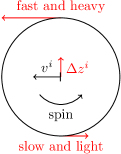
Figure 1: If a spinning spherical symmetric object moves with a velocity $v^{i}$ to the left, then its upper hemisphere moves faster with respect to the observer than its lower hemisphere. Hence, the upper hemisphere possesses a larger relativistic mass than the lower one and the object acquires a mass dipole $S^{i0}=m\Delta z^{i}$. See, e.g., Fleming:1965 .

An interesting, but sometimes problematic, feature of spinning objects in relativity is that their center of mass depends on the observer. This is vividly illustrated in Fig. 1. On the other hand, the definition of the angular momentum of the object, or spin, hinges on the location of the center as the reference point. Hence, both the three-dimensional center and the three-dimensional spin of an object depend on the observer. However, both are combined to form an antisymmetric four-dimensional spin-tensor $S^{\mu\nu}$, where the spatial components $S^{ij}$ contain the usual spin (or flux dipole) and the components $S^{i0}$ give the mass dipole. The latter is non-zero if and only if the observed center of mass differs from the reference point.

Actually, in special relativity, $S^{i0}$ is in one-to-one correspondence with the choice of a reference point. This allows one to represent the choice of center through a condition on $S^{\mu\nu}$, called spin supplementary condition (SSC). For instance, the physical meaning of the Fokker-Tulczyjew condition $S_{\mu\nu}p^{\nu}=0$ Fokker:1929 ; Tulczyjew:1959 is that one observes a vanishing mass dipole $S^{i0}=0$ in the rest-frame of the object, where its momentum $p^{\nu}$ is parallel to the time direction. In other words, the chosen center agrees with the center of mass observed in the rest-frame. Because physically the dynamics of the object must be independent of the reference worldline $z^{\mu}(\sigma)$ we chose to represent its motion, this choice is a gauge choice and the SSC can be understood as a gauge fixing. However, we will see that, in the context of an action formulation for spinning particles, there is a twist in this story. In general relativity, the correspondence between the choice of center and the SSC was rigorously demonstrated only for the special case $S_{\mu\nu}p^{\nu}=0$ Schattner:1979:1 ; Schattner:1979:2 , but intuitively one should expect that it holds more generally, too.

To date, the prototype construction for an action and canonical formalism of classical spinning particles in special relativity is given in a seminal paper of Hanson and Regge Hanson:Regge:1974 . (For earlier work on the action see Goenner:Westpfahl:1967 ; Westpfahl:1969:2 and for the canonical formalism see Kunzle:1972 ). However, this construction essentially covers the choice $S_{\mu\nu}p^{\nu}=0$ only, which has the advantage of being a covariant condition. Then the covariance of the theory is manifest. But following the idea that the choice of a reference worldline can be seen as an arbitrary gauge choice, one would instead expect that the action possesses a corresponding gauge symmetry, so that any SSC can be used equivalently at the level of the action. It is the main purpose of the present paper to work out a recipe for the construction of such a gauge-invariant action in special relativity, and in this sense completes the work in Hanson:Regge:1974 .

It is important to notice that Ref. Hanson:Regge:1974 is the basis of current methods for the computation of general relativistic spin effects in compact binaries Porto:2006 ; Porto:Rothstein:2006 ; Porto:Rothstein:2008:2 ; Levi:2008 ; Steinhoff:Schafer:2009:2 ; Steinhoff:2011 ; Levi:2010 ; Buonanno:Faye:Hinderer:2013 ; Blanchet:Buonanno:LeTiec:2013 ; Marsat:2014 ; Blanchet:2014 . Predictions for these spin effects are of great importance for future gravitational wave astronomy. For instance, some black holes are known to spin rapidly Reynolds:2013 ; McClintock:Narayan:Steiner:2013 and certain spin orientations lead to an increased gravitational wave luminosity Reisswig:Husa:Rezzolla:Dorband:Pollney:Seiler:2009 . This makes it likely that spin effects are relevant for the first detectable sources. If spinning compact objects are modeled through an effective field theory approach (EFT) Porto:2006 ; Levi:2010 ; Goldberger:Rothstein:2006 , then it is vital to implement all expected symmetries in the effective action. However, the gauge symmetry related to the choice of a representative worldline was not considered so far.

It is noteworthy that classical spinning particles are based on a spin-1 representation in the present paper, while Fermions transform under fractional spin representations. But still, an action for classical spinning particles can also be seen as an effective theory for fermion fields in certain limits. The clearest way to understand the classical limit is through a Foldy-Wouthuysen transformation Foldy:Wouthuysen:1950 ; Silenko:2003 . This is a unitary transformation of the spinors, which removes the Zitterbewegung. This unitary representation corresponds to the choice of the Pryce-Newton-Wigner center Pryce:1935 ; Pryce:1948 ; Newton:Wigner:1949 for the representative point in the classical theory. Then the commutators, or Poisson brackets, of the three-dimensional spin and position are the (rather simple) standard canonical ones.

We adopt the conventions from Hanson:Regge:1974 .

II Spinning particles

Before we discuss classical spinning particles, it is useful to recapitulate the definition of particles in quantum theory. One-particle states are defined by the property of transforming under an irreducible representation of the Poincaré group Weinberg:1995 . That is, a particle is still the same one if it is transformed to a different position, orientation, or speed by the Poincaré group and the irreducibility guarantees that it can not be separated into parts, so it is indeed just one particle. The linear momentum of the particle $p_{\mu}$ follows as the eigenvalue of the translation operator. Since $p_{\mu}$ transforms as a vector under Lorentz transformations, it can not label the irreducible representations, but the scalar $p_{\mu}p^{\mu}=\mathcal{M}^{2}$ can. Now, all vectors on such a mass shell are connected by Lorentz transformations, so one can define a standard Lorentz transformation $L(p)$ which brings $p_{\mu}$ to some standard form. A generic Lorentz transformation of the particle state can then be decomposed into the standard Lorentz transformation $L(p)$ and an element of the so called little group. The latter leaves the standard form of $p_{\mu}$ invariant. For instance, for massive particles ($\mathcal{M}^{2}>0$) one usually chooses the standard form of $p_{\mu}$ to point to the time direction ($p_{\mu}$ is boosted to the rest frame) and the little group is the rotation group SO(3) (Wigner rotation), since it leaves the time direction invariant. Finally, this simple group-theoretical definition of particles implies that particles are characterized by a mass shell and an irreducible representation of the little group, which carries a spin quantum number. An analogous group-theoretical approach can be used in the classical context Bel:Martin:1980 .

For classical particles, we follow Hanson:Regge:1974 and represent the configuration space of the particle by a position $z^{\mu}$ and a Lorentz matrix $\Lambda_{A}{}^{\mu}$, with obvious transformation properties under the Poincaré group. Here the index $A$ labels the basis of the body-fixed frame. Though this is borrowing terminology from a rigid body, we insist that the constructed action can serve as an effective description of generic spinning bodies. The generators of the Poincaré group are the linear momentum $p_{\mu}$ and the total angular momentum $J_{\mu\nu}=2z_{[\mu}p_{\nu]}+S_{\mu\nu}$, so the Poisson brackets must read

$$\{z^{\mu},p_{\nu}\} =\delta^{\mu}_{\nu},\quad\{\Lambda_{A}{}^{\alpha},S_{\mu\nu}\}=2\Lambda_{A}{}^{\beta}\eta_{\beta[\mu}\delta^{\alpha}_{\nu]},$$ (1)

$$\{S_{\alpha\beta},S_{\mu\nu}\} =S_{\alpha\mu}\eta_{\nu\beta}-S_{\alpha\nu}\eta_{\mu\beta}+S_{\beta\nu}\eta_{\mu\alpha}-S_{\beta\mu}\eta_{\nu\alpha},$$

all other zero, where $\eta_{\mu\nu}$ is the Minkowski metric.

We consider the case of a massive particle here. Then we can define a standard boost which transforms the time direction of the body-fixed frame $\Lambda_{0}{}^{\mu}$ into the direction of the linear momentum $p_{\mu}$,

$$L^{\mu}{}_{\nu}=\delta^{\mu}{}_{\nu}+2\frac{p^{\mu}\Lambda_{0\nu}}{p}-\frac{p\omega^{\mu}\omega_{\nu}}{p_{\rho}\omega^{\rho}},$$ (2)

where $p:=\sqrt{p_{\mu}p^{\mu}}$ and for later convenience we have introduced the time-like vector $\omega^{\nu}:=p^{\nu}/p+\Lambda_{0}{}^{\nu}$. When applied to the Lorentz matrix, we obtain a new matrix $\tilde{\Lambda}_{A}{}^{\mu}=L^{\mu}{}_{\nu}\Lambda_{A}{}^{\nu}$, or explicitly

$$\tilde{\Lambda}_{0}{}^{\mu}=\frac{p^{\mu}}{p},\quad\tilde{\Lambda}_{i}{}^{\mu}=\Lambda_{i}{}^{\mu}-\Lambda_{i}{}^{\nu}\frac{p_{\nu}\omega^{\mu}}{p_{\rho}\omega^{\rho}}.$$ (3)

We notice that $\tilde{\Lambda}_{0}{}^{\mu}$ is redundant, since it is given by $p_{\mu}$. The independent physical degrees of freedom are contained in $\tilde{\Lambda}_{i}{}^{\mu}$, which carries an SO(3) index and hence transforms under the vector (spin-1) representation of the little group. This is intuitively clear, since the state of motion is already characterized by the linear momentum and the temporal component of the body-fixed frame must be redundant. The physical information of the body-fixed frame is the orientation of the object, which should be associated with three-dimensional rotations.

Because $\Lambda_{A}{}^{\mu}$ contains irrelevant, or gauge, degrees of freedom, its conjugate $S_{\mu\nu}$ must be subject to a constraint. This constraint is usually also the generator of the gauge symmetry Pons:2005 , which must leave the physical degrees of freedom $\tilde{\Lambda}_{i}{}^{\mu}$ invariant. From the projector-like structure of Eq. (3) and the fact that the spin generates Lorentz transformations of $\Lambda_{i}{}^{\mu}$, we may guess that the generator is given by $S_{\mu\nu}\omega^{\nu}$. Indeed, we find

$$\{S_{\mu\nu}\omega^{\nu},\tilde{\Lambda}_{i}{}^{\rho}\}=0,$$ (4)

where we made use of $\omega^{\mu}p_{\mu}/p=\omega_{\mu}\Lambda_{0}{}^{\mu}=\frac{1}{2}\omega_{\mu}\omega^{\mu}$ and $\tilde{\Lambda}_{i}{}^{\mu}w_{\mu}=\tilde{\Lambda}_{i}{}^{\mu}p_{\mu}$. We have discovered the spin gauge constraint

$$0\approx\mathcal{C}_{\mu}:=S_{\mu\nu}\left(\frac{p^{\nu}}{p}+\Lambda_{0}{}^{\nu}\right)\equiv S_{\mu\nu}\omega^{\nu},$$ (5)

where weak equality Dirac:1964 (restriction to the constraint surface) is denoted by $\approx$. It is further illustrated below that this constraint physically makes sense. This spin gauge constraint is not an SSC (in the usual sense) and does not correspond to a choice for the worldline, but it parametrizes the possible SSCs through a gauge field $\Lambda_{0}{}^{\nu}$, see below for discussion.

We notice that Ref. Hanson:Regge:1974 was missing the $\Lambda_{0}{}^{\nu}$ in this constraint. One might object that the appearance of $\Lambda_{0}{}^{\nu}$ is breaking the SO(1,3) Lorentz invariance in its first index. However, this index belongs to the body-fixed frame, whose time-like component is not an observable. Indeed, we already argued that $\Lambda_{0}{}^{\nu}$ is a physically irrelevant gauge degree of freedom. Furthermore, also from an EFT point of view, only SO(3) rotation invariance is a symmetry that must be respected for the body-fixed frame Goldberger:2007 ; Goldberger:Rothstein:2006 , instead of SO(1,3) Lorentz invariance.

We must have another constraint related to a gauge symmetry here, namely that of reparametrization invariance of the worldline parameter $\sigma$. The associated constraint is the mass shell one Hanson:Regge:1974

$$0\approx\mathcal{H}:=p_{\mu}p^{\mu}-\mathcal{M}^{2},$$ (6)

which together with (5) forms the basis for an action principle.

III Action for spinning particles

We are going to construct an action principle based on a Hamiltonian. The Dirac Hamiltonian $H_{D}$ Rosenfeld:1930 ; Dirac:1964 ; Pons:2005 is the canonical Hamiltonian plus the (primary) constraints, which are added with the help of Lagrange multipliers. However, due to reparametrization invariance, the canonical Hamiltonian vanishes, so that $H_{D}$ is just composed of the constraints,

$$H_{D}=\frac{\lambda}{2}\mathcal{H}+\chi^{\mu}\mathcal{C}_{\mu},$$ (7)

where $\lambda$ and $\chi^{\mu}$ are the Lagrange multipliers.

An action principle for spinning point-particles (PP) must reproduce the equations of motion of $H_{D}$ with Poisson brackets from Eq. (1). The relation between action and Poisson brackets is discussed in Appendix A. The appropriate action reads Hanson:Regge:1974

$$S_{\text{PP}}=\int d\sigma\left[-p_{\mu}u^{\mu}-\frac{1}{2}S_{\mu\nu}\Omega^{\mu\nu}-H_{D}\right],$$ (8)

where the variables with independent variations are $z^{\mu}$, $p_{\mu}$, $\Lambda^{A\mu}$, and $S_{\mu\nu}$ and we introduced the abbreviations $u^{\mu}=\dot{z}^{\mu}$, $\Omega^{\mu\nu}=\Lambda_{A}{}^{\nu}\dot{\Lambda}^{A\mu}$, and $\dot{~{}}=d/d\sigma$. Since $\Lambda^{A\mu}$ is a Lorentz matrix, it can only be varied by an infinitesimal Lorentz transformation $\delta\theta^{\mu\nu}=-\delta\theta^{\nu\mu}$, i.e., $\delta\Lambda^{A\mu}=\Lambda^{A\nu}\delta\theta_{\nu}{}^{\mu}$.

Notice that the dynamical mass $\mathcal{M}$ can be a general function of the dynamical variables. Then the mass $\mathcal{M}$ contains all the interaction energies. It must be adapted such that the point-particle provides an effective description for some extended body on macroscopic scale (reducing the almost innumerable internal degrees of freedom of the body to the relevant ones). The dynamics is then encoded through $\mathcal{M}$ and the action principle. This makes the dynamical mass $\mathcal{M}$ analogous to a thermodynamic potential, like the internal energy. It should be noted that EFTs are of comparable importance for both particle and statistical physics. The analogy of $\mathcal{M}$ to a thermodynamic potential suggests to apply a construction of $\mathcal{M}$ using symmetries and power counting arguments, as usual in an EFT. For black holes, $\mathcal{M}$ as a function of the dynamical variables is related to the famous laws of black hole dynamics Misner:Thorne:Wheeler:1973 , see also Steinhoff:2014:2 for discussion.

We require here that the constraints in $H_{D}$ are related to gauge symmetries. Then the Lagrange multipliers are not fixed by requiring that the constraints are preserved in time and represent the gauge freedom. This implies that the Poisson brackets between all pairs of constraints vanish weakly here. Constraints with this property are called first class Dirac:1964 . See Ref. Pons:2005 for further discussion of gauge symmetry in constrained Hamiltonian dynamics. In contrast to our requirement that all three independent components of the spin constraints are first class, only one component of the spin constraint used in Hanson:Regge:1974 is first class. This renders the completion of the set of constraints in Hanson:Regge:1974 rather unsatisfactory, because only first class constraints require a completion through gauge fixing constraints.

IV Spin gauge constraint

The first main objective of the present paper is to establish $\mathcal{C}_{\mu}$ as the proposed spin gauge constraint. We just argued that it should be a first class constraint. Furthermore, it should be the generator of a spin gauge transformation, i.e., a shift of the representative worldline $\Delta z^{\mu}(\sigma)$ together with the appropriate change in the spin,

$$\Delta S_{\mu\nu}\approx 2p_{[\mu}\Delta z_{\nu]},$$ (9)

This is in agreement with the physical picture in Fig. 1, which refers to the rest-frame where $p^{\mu}=(m,0)$. These are the physical requirements we have on $\mathcal{C}_{\mu}$.

These requirements are indeed met for Eq. (5). It is easy to see that $\mathcal{C}_{\mu}$ is first-class among itself,

$$\{\mathcal{C}_{\mu},\mathcal{C}_{\nu}\}=\frac{2}{p}p_{[\mu}\mathcal{C}_{\nu]}\approx 0,$$ (10)

so it qualifies for a gauge constraint. Then the generator of an infinitesimal spin gauge transformation is $\epsilon^{\mu}\mathcal{C}_{\mu}$ and the transformations of the fundamental variables read

$$\Delta z^{\mu} :=\{\epsilon^{\alpha}\mathcal{C}_{\alpha},z^{\mu}\}=\frac{1}{p}P^{\mu\nu}S_{\nu\alpha}\epsilon^{\alpha},$$ (11)

$$\Delta p^{\mu} :=\{\epsilon^{\alpha}\mathcal{C}_{\alpha},p^{\mu}\}=0,$$ (12)

$$\Delta\Lambda_{A}{}^{\mu} :=\{\epsilon^{\alpha}\mathcal{C}_{\alpha},\Lambda_{A}{}^{\mu}\}=2\epsilon^{[\mu}\omega^{\nu]}\Lambda_{A\nu},$$ (13)

$$\Delta S_{\mu\nu} :=\{\epsilon^{\alpha}\mathcal{C}_{\alpha},S_{\mu\nu}\}=2p_{[\mu}\Delta z_{\nu]}-2\epsilon_{[\mu}\mathcal{C}_{\nu]},$$ (14)

where $P^{\mu\nu}$ is the projector onto the spatial hypersurface of the rest-frame,

$$P^{\mu\nu}:=\eta^{\mu\nu}-\frac{p^{\mu}p^{\nu}}{p^{2}}.$$ (15)

Notice that $\Delta z^{\mu}$ is a spatial vector in the rest-frame of the particle, $p_{\mu}\Delta z^{\mu}=0$. This makes it obvious that the symmetry group is three-dimensional.

Now, on the constraint surface, Eq. (14) is identical to our second and final requirement in Eq. (9). That is, it is precisely the amount that an angular momentum changes if the reference point is moved by $\Delta z^{\mu}$. This shows that $\epsilon^{\mu}\mathcal{C}_{\mu}$ indeed generates a shift of the reference worldline within the object and that $\mathcal{C}_{\mu}$ is the corresponding gauge constraint.

While the physical meaning of $\Delta S_{\mu\nu}$ is immediately clear, an interpretation of $\Delta\Lambda_{A}{}^{\mu}$ deserves a more detailed illustration. We recall that the physically relevant components of $\Lambda_{A}{}^{\mu}$ are obtained by a finite boost to the rest frame, see Eq. (2). Therefore, $\Delta\Lambda_{A}{}^{\mu}$ should be given by a standard boost to the rest-frame followed by another standard boost to a frame infinitesimally close to $\Lambda^{A\mu}$. It is straightforward to check using the standard boost, Eq. (2), that this is the case.

V Spin gauge fixing

As usual, a gauge fixing now requires a gauge condition, that is, a condition on the gauge field $\Lambda_{0}{}^{\mu}$. Notice that the spin gauge constraint (5) does not correspond to a choice for a representative worldline, because it contains the unspecified gauge field $\Lambda_{0}{}^{\mu}$. The following choices turn the spin gauge constraint (5) into familiar choices for the SSC:

$$\Lambda_{0}{}^{\mu} \approx\frac{p^{\mu}}{p}\quad\Rightarrow\quad\mathcal{C}_{\mu}=S_{\mu\nu}p^{\nu}\approx 0,$$ (16)

$$\Lambda_{0}{}^{\mu} \approx\delta_{0}^{\mu}\quad\Rightarrow\quad\mathcal{C}_{\mu}=S_{\mu\nu}(p^{\nu}+p\delta_{0}^{\nu})\approx 0,$$ (17)

$$\Lambda_{0}{}^{\mu} \approx\frac{2p^{0}\delta_{0}^{\mu}-p^{\mu}}{p}\quad\Rightarrow\quad\mathcal{C}_{\mu}=S_{\mu 0}\approx 0.$$ (18)

The first one is due to Fokker Fokker:1929 , the second due to Pryce, Newton, and Wigner Pryce:1935 ; Pryce:1948 ; Newton:Wigner:1949 , and the last one due to Pryce and Møller Pryce:1948 ; Moller:1949 . In general relativity, the first condition was first considered by W. M. Tulczyjew Tulczyjew:1959 , the third one by Corinaldesi and Papapetrou Corinaldesi:Papapetrou:1951 , and the second one was applied more recently only Porto:Rothstein:2006 ; Levi:2008 ; Steinhoff:Schafer:Hergt:2008 ; Barausse:Racine:Buonanno:2009 in slightly different forms and contexts. The differences arise in the way the (normalized) time vector $\delta_{0}^{\mu}$ is generalized to curved spacetime. However, it should be noted that Porto:Rothstein:2006 ; Levi:2008 ; Barausse:Racine:Buonanno:2009 suggest to complete the set of constraints by $\Lambda_{0}{}^{\mu}\propto p^{\mu}$, while here in the context of spin gauge symmetry this would lead to the first SSC, but not to the second one. The SSC and the condition on $\Lambda_{0}{}^{\mu}$ can not be chosen independently here.

Any of the above conditions can be added to the set of constraints, e.g., $0\approx\Lambda_{0}{}^{\mu}-\delta_{0}^{\mu}$. This constraint then turns the spin gauge constraint into a second class constraint, which means that the set of constraints can be eliminated using the Dirac bracket Dirac:1964 (and one can solve for the Lagrange multipliers). This is the usual manner in which gauge fixing is handled in the context of constrained Hamiltonian dynamics.

However, one can alternatively insert the solution to the set of constraints into the action in a classical context. For the case of the Pryce-Newton-Wigner spin gauge, it holds $\Lambda_{0}{}^{\mu}=\delta_{0}^{\mu}$ and $\Lambda_{A}{}^{0}=\delta_{A}^{0}$, so the temporal components drop out of the spin kinematic term in the action,

$$\frac{1}{2}S_{\mu\nu}\Omega^{\mu\nu}=\frac{1}{2}S_{ij}\Omega^{ij},\quad\Omega^{ij}=-\Lambda^{ki}\dot{\Lambda}^{kj}.$$ (19)

The kinematic term still has the same form as in Eq. (8), but the indices are 3-dimensional now and the SO(1,3) Lorentz matrix was reduced to a SO(3) rotation matrix. Therefore, the standard so(1,3) Lie algebra Poisson bracket for the spin, Eq. (1), must be replaced by a standard so(3) algebra for the spatial components of the spin. However, for other gauge choices, the kinematic term will not simplify this drastically and the reduced Poisson bracket algebra will in general be more complicated. This makes the Pryce-Newton-Wigner gauge probably the most useful one if one aims at a reduction of variables, while the Fokker-Tulczyjew one leads to manifestly covariant equations of motion. It should be emphasized that all gauges lead to equivalent equations of motion by construction here, if the mass shell constraint $\mathcal{H}$ is spin gauge invariant.

Note that we obtain the same set of constraints as Hanson:Regge:1974 if we choose the first gauge. However, adding a gauge symmetry to the theory should not be seen as adding unnecessary complications. On the contrary, different gauges are useful for different applications. For instance, in Ref. Hanson:Regge:1974 a transformation from Fokker-Tulczyjew to Pryce-Newton-Wigner variables is considered because it simplifies the reduced Poisson brackets. Here one can directly use the second gauge fixing condition instead and the simplification of brackets is explained by Eq. (19). This is an important consequence of our construction: Different SSCs are manifestly equivalent, in particular the covariant SSC is equivalent to noncovariant ones by construction.

VI Gauge invariant variables

Now we turn to the second main objective of the present paper, which is the construction of the mass shell constraint $\mathcal{H}$ such that it is invariant under spin gauge transformations. This is equivalent to

$$\{\mathcal{C}_{\mu},\mathcal{H}\}\approx 0.$$ (20)

The usual way to construct invariant quantities is by combining objects with are invariant. That is, we aim to find a position, spin, and Lorentz matrix which have weakly vanishing Poisson bracket with $\mathcal{C}_{\mu}$. We already encountered the invariant Lorentz matrix $\tilde{\Lambda}_{i}{}^{\mu}$ given by Eq. (3). Recalling that $\tilde{\Lambda}_{i}{}^{\mu}$ was obtained by a boost to the rest frame, we may guess that the following projections to the rest-frame variables,

$$\tilde{z}^{\mu}:=z^{\mu}+S^{\mu\nu}\frac{p_{\nu}}{p^{2}},\quad\tilde{S}_{\mu\nu}:=P_{\mu}{}^{\alpha}P_{\nu}{}^{\beta}S_{\alpha\beta}$$ (21)

have the desired properties. It is indeed straightforward to show that these variables with a tilde have weakly vanishing Poisson brackets with $\mathcal{C}_{\mu}$,

$$\{\mathcal{C}_{\alpha},\tilde{z}^{\mu}\} =-\frac{1}{p^{2}}[\delta^{\mu}_{\alpha}p_{\nu}-\delta^{\mu}_{\nu}p_{\alpha}]\mathcal{C}^{\nu}\approx 0,$$ (22)

$$\{\mathcal{C}_{\alpha},\tilde{S}_{\mu\nu}\} =-2P_{\alpha[\mu}P_{\nu]}{}^{\beta}\mathcal{C}_{\beta}\approx 0,$$ (23)

and the linear momentum is already invariant, see Eq. (12). Therefore, if the mass shell constraint depends on these variables only, then it is invariant under spin gauge transformation,

$$\mathcal{M}=\mathcal{M}(\tilde{z}^{\mu},p^{\mu},\tilde{\Lambda}_{i}{}^{\mu},\tilde{S}_{\mu\nu})\quad\Rightarrow\quad\{\mathcal{C}_{\mu},\mathcal{H}\}\approx 0.$$ (24)

The most simple model is given by

$$\mathcal{M}^{2}=f(\tilde{S}^{2})\quad\text{in}\quad\mathcal{H}=p_{\mu}p^{\mu}-\mathcal{M}^{2},$$ (25)

and $\tilde{S}^{2}=\frac{1}{2}\tilde{S}_{\mu\nu}\tilde{S}^{\mu\nu}$. Here $f$ is an almost arbitrary function, commonly referred to as a Regge trajectory Hanson:Regge:1974 . We require it to be analytic and nonconstant (for $f=\text{const}$ it follows $\Omega^{\mu\nu}=0$ for any spin). This function encodes the rotational kinetic energy and the moment of inertia of the body. For black holes, it is related to the laws of black hole mechanics.

VII Simplified invariant action

The construction of the last section has a problematic aspect. All fields interactions, entering through the dynamical mass $\mathcal{M}$, must be taken at the position $\tilde{z}^{\mu}$, which in general is different from the worldline coordinate $z^{\mu}$. This is particularly a problem for coupling to the gravitational field, because first of all the tangent spaces at $\tilde{z}^{\mu}$ and $z^{\mu}$ are different and second the difference between the positions is not a tangent vector. Therefore, it is not straightforward to generalize the current construction to the general relativistic case, where the dynamical mass must be coordinate invariant.

However, because the mass shell constraint must be written entirely in terms of the position $\tilde{z}^{\mu}$, it is suggestive to shift the worldine of the action to this position. It should be noted that one can not switch to the invariant spin and Lorentz matrix as fundamental variables, because the transformation involves projections (notice $\tilde{\Lambda}_{i}{}^{\mu}p_{\mu}=0$). This leads to an action containing a time derivative of the momentum,

$$S_{\text{PP}}=\int d\sigma\left[-p_{\mu}\tilde{u}^{\mu}-S^{\mu\nu}\frac{\dot{p}_{\mu}p_{\nu}}{p^{2}}-\frac{1}{2}S_{\mu\nu}\Omega^{\mu\nu}-H_{D}\right].$$ (26)

The Poisson brackets involving $\tilde{z}^{\mu}$ will not be standard canonical, but they can be readily obtained from Eq. (21) and the old Poisson brackets. Note that one can associate Poisson brackets to an action if it contains at most first order time derivatives (and no pathologies arise). See the Appendix A. The equations of motion are still first order, which is important because otherwise more initial values would be needed.

Now it is now straightforward to couple the spinning particle to the gravitational field, namely by replacing ordinary derivatives with respect to $\sigma$ in Eq. (26) by covariant ones (minimal coupling). Additionally, nonminimal couplings can be added in the sense of an effective theory via the dynamical mass $\mathcal{M}$, as long as these are evaluated at the position of the new worldline $\tilde{z}^{\mu}$ and constructed using the matter variables $\tilde{\Lambda}_{i}{}^{\mu}$, $\tilde{S}_{\mu\nu}$, and $p_{\mu}$. Further development of the general relativistic case and an application to the post-Newtonian approximation is given in Levi:Steinhoff:2014:3 . In the following section, we illustrate that this construction is also convenient for coupling to other fields, like the electromagnetic one, and see that nonminimal couplings represent the multipoles of the body Bailey:Israel:1975 ; Porto:Rothstein:2008:2 ; Levi:Steinhoff:2014:2 .

The time derivative of the momentum in our action is similar to the acceleration term introduced in Yee:Bander:1993 . (It also appeared in a similar time+space decomposed form in Hergt:Steinhoff:Schafer:2011 ; Levi:Steinhoff:2014:1 .) After a coupling to gravity (or the electromagnetic field), one can approximately remove this term, if this is desired, using a manifestly covariant shift of the worldline as introduced in Bailey:Israel:1980 . This approximately corresponds to inserting the equation of motion for $\dot{p}_{\mu}$ into the action Damour:Schafer:1991 . This transformation leads to the nonminimal coupling proportional to the Fokker-Tulczyjew SSC used in Porto:Rothstein:2008:2 . However, in both Refs. Yee:Bander:1993 ; Porto:Rothstein:2008:2 this term was introduced in order to preserve the covariant SSC, while here it arises from the requirement of spin gauge symmetry. This distinction is significant in the context of an EFT.

VIII Electromagnetic interaction

A minimal coupling to the electromagnetic field with charge $q$ can be introduced as usual by adding $-q\tilde{A}_{\mu}\tilde{u}^{\mu}$ to the Lagrangian, see, e.g., Eq. (6.1) in Arnowitt:Deser:Misner:1962 ; Arnowitt:Deser:Misner:2008 ,

$$S_{\text{PP}} =\int d\sigma\bigg{[}-p_{\mu}\tilde{u}^{\mu}-q\tilde{A}_{\mu}\tilde{u}^{\mu}$$

$$\quad-S^{\mu\nu}\frac{\dot{p}_{\mu}p_{\nu}}{p^{2}}-\frac{1}{2}S_{\mu\nu}\Omega^{\mu\nu}-H_{D}\bigg{]},$$ (27)

where $\tilde{A}_{\mu}=A_{\mu}(\tilde{z}^{\nu})$. This new term turns into a total time derivative under electromagnetic gauge transformations. The added term is also manifestly invariant under spin gauge transformations, because it only involves invariant quantities. Here it is convenient that we shifted the worldline to the spin-gauge-invariant position $\tilde{z}^{\mu}$.

We are going to derive the equations of motion belonging to the action (VIII) and explicitly construct the Poisson brackets associated to it. The $\delta p_{\mu}$-variation leads to the velocity-momentum relation

$$\begin{split}\tilde{u}^{\mu}&=2\tilde{S}^{\mu\nu}\frac{\dot{p}_{\nu}}{p^{2}}+\dot{S}^{\mu\nu}\frac{p_{\nu}}{p^{2}}-\frac{\partial H_{D}}{\partial p_{\mu}},\end{split}$$ (28)

and from the $\delta S_{\mu\nu}$-variation it follows

$$\begin{split}\Omega^{\mu\nu}&=\frac{2p^{[\mu}\dot{p}^{\nu]}}{p^{2}}-2\frac{\partial H_{D}}{\partial S_{\mu\nu}}.\end{split}$$ (29)

Finally, the $\delta\tilde{z}^{\mu}$-variation leads to

$$\begin{split}\dot{p}_{\mu}=-q\tilde{F}_{\mu\nu}\tilde{u}^{\nu}+\frac{\partial H_{D}}{\partial\hat{z}^{\mu}},\end{split}$$ (30)

with the Faraday tensor $\tilde{F}_{\mu\nu}:=\tilde{A}_{\mu,\nu}-\tilde{A}_{\nu,\mu}$, and the $\delta\Lambda^{A\mu}$-variation gives

$$\begin{split}\dot{S}_{\mu\nu}=-2\Omega^{\rho}{}_{[\mu}S_{\nu]\rho}+2\Lambda_{A[\mu}\frac{\partial H_{D}}{\partial\Lambda_{A}{}^{\nu]}},\end{split}$$ (31)

We eliminate the time derivatives on the right hand side of Eq. (28),

$$\tilde{u}^{\mu} =-\frac{q}{p^{2}}\tilde{S}^{\mu\nu}\tilde{F}_{\nu\alpha}\tilde{u}^{\alpha}+U^{\mu},$$ (32)

$$\begin{split}U^{\mu}&:=-\frac{\partial H_{D}}{\partial p_{\mu}}-4\delta_{\alpha}^{[\mu}S^{\nu]}{}_{\beta}\frac{p_{\nu}}{p^{2}}\frac{\partial H_{D}}{\partial S_{\alpha\beta}}\\ &\quad+\frac{\tilde{S}^{\mu\nu}}{p^{2}}\frac{\partial H_{D}}{\partial\hat{z}^{\nu}}+2\frac{\eta^{\mu[\alpha}p^{\nu]}}{p^{2}}\Lambda_{A\alpha}\frac{\partial H_{D}}{\partial\Lambda_{A}{}^{\nu}},\end{split}$$ (33)

which can be solved for $\tilde{u}^{\mu}$ using Eq. (A.4) and (A.7) in Ref. Hanson:Regge:1974 ,

$$\tilde{u}^{\mu}=\left[\delta_{\alpha}^{\mu}-\frac{q\tilde{S}^{\mu\nu}\tilde{F}_{\nu\alpha}}{p^{2}-\frac{1}{2}q\tilde{S}^{\rho\delta}\tilde{F}_{\rho\delta}}\right]U^{\alpha},$$ (34)

where we used $\tilde{S}_{\mu\nu}*\!\tilde{S}^{\mu\nu}=0$ ($*$ denotes the Hodge dual). Using this relation, all time derivatives can be removed from the right hand sides of the equations of motion. The equation of motion of a dynamical variable is then expressed in terms of derivatives of $H_{D}$ with respect to other dynamical variables only, and the prefactor is the mutual Poisson bracket. Explicit expressions for all Poisson brackets are given in Appendix A. These Poisson brackets are similar to Eq. (5.29) in Hanson:Regge:1974 . However, for most applications it should be sufficient to have an action principle and the equations of motion in the form given above. But it is good to know that the equations of motion follow a symplectic flow and that the Poisson brackets can be obtained explicitly if needed. An analogous calculation should be possible for the gravitational interaction.

The finite-size and internal structure of the particle is modelled by nonminimal couplings in the dynamical mass $\mathcal{M}$. These are composed of the (electromagnetic gauge invariant) Faraday tensor $F_{\mu\nu}$ and its derivatives, where an increasing number of derivatives corresponds to smaller length scales or higher multipoles. As an illustration for the treatment of electromagnetic multipoles, we consider the simplest case of a dipole, which corresponds to a nonminimal coupling to the Faraday tensor $F_{\mu\nu}$ in the dynamical mass. For a spin-induced dipole, this reads

$$\mathcal{M}^{2}=f(\tilde{S}^{2})+\frac{gq}{2}\tilde{F}_{\mu\nu}\tilde{S}^{\mu\nu},$$ (35)

where $g$ is the gyromagnetic ratio. For this model, our equations of motion are in agreement with Hanson:Regge:1974 . Making the gauge choice $\Lambda_{0}{}^{\mu}=p^{\mu}/p$ and requiring that it is preserved in time by above equations of motions, we find that $\chi^{\mu}=0$ for the Lagrange multiplier of the spin gauge constraint in this case. A contraction of (28) with $p_{\mu}$ then leads to $\lambda=\tilde{u}^{\mu}p_{\mu}/p^{2}$ for the Lagrange multiplier of the mass shell constraint, which is related to the parametrization of the worldline. Then we find structural agreement with (4.29), (4.33), and (4.34) in Hanson:Regge:1974 and therefore also with the Bargmann-Michel-Telegdi equations Bargmann:Michel:Telegdi:1959 . The normalization of the dipole interaction differs compared to Hanson:Regge:1974 , which is due to the fact that in Hanson:Regge:1974 the dipole is proportional to the angular velocity, while here it is proportional to the spin. In Bargmann:Michel:Telegdi:1959 the SSC $S^{\mu\nu}u_{\mu}=0$ Frenkel:1926 ; Mathisson:1937 ; Mathisson:2010 is used, which fails to uniquely define a worldline and in general leads to helical motion Mathisson:1937 ; Mathisson:2010 ; Costa:etal:2011 . Finally, we notice that a dipole linearly induced by an external field is modelled by couplings of the form shown in Eq. (1) of Ref. Goldberger:Rothstein:2006:2 , which can be added to the dynamical mass here.

If desired, one can shift the $\dot{p}_{\mu}$-term in the action (VIII) to higher orders in the derivative of the electromagnetic field through redefinitions of the variables Damour:Schafer:1991 . That is, through successive redefinitions, one can turn the $\dot{p}_{\mu}$-term into nonminimal interaction terms of increasing derivative order. Consistent with neglecting finite-size effects of a certain multipolar order in $\mathcal{M}$, one can terminate this process at the desired order and the $\dot{p}_{\mu}$-term is effectively removed. The physical reason for the additional nonminimal interactions is that a shift of position of a monopole $q$ generates an infinite series of higher multipoles Bailey:Israel:1980 .

IX Conclusions

The spin gauge symmetry formulated in the present paper is an important ingredient to extend the EFT for charged particles to spinning charged particles (see, e.g., Galley:Leibovich:Rothstein:2010 ). This should serve as a classical EFT for massive fermions. Massless particles have a different little group, so our approach need several adjustments for this case. We identified spin gauge invariant variables in the present paper, which should be useful for a matching of the EFT.

The general relativistic case is analogous to the electromagnetic one and is invaluable for modelling the motion of black holes and neutron stars. This will lead to better gravitational wave forms needed for the data analysis requirements of future gravitational wave astronomy.

Appendix A Poisson brackets from the action

Consider an action containing at most first order derivatives in time. We can write it in the form

$$S=\int dt\left[B_{a}(q^{b})\,\dot{q}^{a}-H(q^{b})\right],$$ (36)

where $a$, $b$ label the dynamical variables $q_{a}$. The equations of motion read

$$M_{ab}\dot{q}^{b}=\partial_{a}H,\quad M_{ab}:=\partial_{a}B_{b}-\partial_{b}B_{a}.$$ (37)

where $\partial_{a}=\partial/\partial q^{a}$, or

$$\dot{q}^{a}=M^{ab}\partial_{b}H,\quad M^{ab}:=M_{ab}^{-1}$$ (38)

This can be written using Poisson brackets

$$\dot{q}^{a}=\{H,q^{a}\},$$ (39)

if we set

$$\{X,Y\}=M^{ba}\partial_{a}X\partial_{b}Y.$$ (40)

Instead of computing $M_{ab}$ and its inverse directly from the action, it is often easier to obtain the equations of motion and transform them to the form of Eq. (38). Then one can directly read off $M_{ab}^{-1}$. For the case of electromagnetically interacting spinning particles (VIII), we have $\tilde{u}^{\mu}=G^{\mu}{}_{\nu}U^{\nu}$ where

$$G^{\mu}{}_{\nu}=\delta_{\nu}^{\mu}-\frac{q}{P^{2}}\tilde{S}^{\mu\alpha}\tilde{F}_{\alpha\nu},\quad P^{2}=p^{2}-\frac{1}{2}q\tilde{S}^{\mu\nu}\tilde{F}_{\mu\nu}.$$ (41)

This leads to the Poisson brackets involving $\tilde{z}^{\mu}$

$$\{\hat{z}^{\mu},\tilde{z}^{\nu}\} =G^{\nu}{}_{\alpha}\frac{\tilde{S}^{\alpha\mu}}{p^{2}}=-\frac{\tilde{S}^{\mu\nu}}{P^{2}},$$ (42)

$$\{p_{\mu},\tilde{z}^{\nu}\} =-G^{\nu}{}_{\mu},$$ (43)

$$\{\Lambda_{A}{}^{\mu},\tilde{z}^{\nu}\} =\frac{2}{p^{2}}G^{\nu[\alpha}p^{\mu]}\Lambda_{A\alpha},$$ (44)

$$\{S_{\mu\nu},\tilde{z}^{\alpha}\} =-\frac{4}{p^{2}}G^{\alpha}{}_{\beta}\delta^{[\beta}_{[\mu}S^{\rho]}{}_{\nu]}p_{\rho},$$ (45)

where we used Eq. (A.5) in Hanson:Regge:1974 ,

$$G^{\nu}{}_{\alpha}\frac{\tilde{S}^{\alpha\mu}}{p^{2}}=-\frac{\tilde{S}^{\mu\nu}}{P^{2}}=-G^{\mu}{}_{\alpha}\frac{\tilde{S}^{\alpha\nu}}{p^{2}}.$$ (46)

Similarly, from considering the equation of motion for $p_{\mu}$,

$$\{p_{\mu},p_{\nu}\} =q\tilde{F}_{\nu\alpha}G^{\alpha}{}_{\mu},$$ (47)

$$\{\Lambda_{A}{}^{\mu},p_{\nu}\} =-\frac{2q}{p^{2}}\tilde{F}_{\nu\beta}G^{\beta[\alpha}p^{\mu]}\Lambda_{A\alpha},$$ (48)

$$\{S_{\mu\nu},p_{\alpha}\} =\frac{4q}{p^{2}}\tilde{F}_{\alpha\delta}G^{\delta}{}_{\beta}\delta^{[\beta}_{[\mu}S^{\rho]}{}_{\nu]}p_{\rho},$$ (49)

and from the remaining equations

$$\{\Lambda_{A}{}^{\mu},\Lambda_{B}{}^{\nu}\} =-\frac{4q}{p^{4}}\Lambda_{B\rho}p^{[\rho}\tilde{F}^{\nu]}{}_{\beta}G^{\beta[\alpha}p^{\mu]}\Lambda_{A\alpha},$$ (50)

$$\begin{split}\{S_{\mu\nu},\Lambda_{A}{}^{\alpha}\}&=-2\Lambda_{A}{}^{\beta}\eta_{\beta[\mu}\delta^{\alpha}_{\nu]}\\ &\quad+\frac{8q}{p^{4}}\Lambda_{A\delta}p^{[\delta}\tilde{F}^{\alpha]}{}_{\sigma}G^{\sigma}{}_{\beta}\delta^{[\beta}_{[\mu}S^{\rho]}{}_{\nu]}p_{\rho},\end{split}$$ (51)

$$\begin{split}\{S_{\mu\nu},S_{\alpha\beta}\}&=-4S_{\alpha][\mu}\eta_{\nu][\beta}\\ &\quad+\frac{16q}{p^{4}}S^{\gamma}{}_{[\alpha}\delta_{\beta]}^{\delta}p_{[\delta}\tilde{F}_{\gamma]\sigma}G^{\sigma}{}_{\chi}\delta^{[\chi}_{[\mu}S^{\rho]}{}_{\nu]}p_{\rho}.\end{split}$$ (52)

The Poisson brackets are rather complicated. For most applications, it is therefore better to work directly with the action (VIII) if possible.

Appendix B Another check against Ref. Hanson:Regge:1974

The term involving $\dot{p}_{\mu}$ in Eq. (VIII) can be removed by variable redefinitions, which will then be canonical variables because the action assumes a canonical form. Here we only intend to make a connection to the results in Hanson:Regge:1974 . Therefore we apply the gauge fixing $\Lambda_{0}{}^{\mu}=p^{\mu}/p$, or the SSC $S_{\mu\nu}p^{\mu}=0$. The term containing $\dot{p}_{\mu}$ can be cancelled from the action by shifting back to the position $z^{\mu}$. Now new contributions arise from the minimal coupling term. However, at the level of the action, we can neglect terms of quadratic or higher order in the SSC $S_{\mu\nu}p^{\mu}$. Then one can absorb all additional terms by defining the canonical momentum

$$p_{\mu}^{\text{can}}=p_{\mu}+qA_{\mu}+qF_{\mu\nu}S^{\nu\rho}\frac{p_{\rho}}{p^{2}}.$$ (53)

This can be solved for $p_{\mu}$ using the identities in Appendix A of Hanson:Regge:1974 and one finds agreement of (25) with (5.18) in Hanson:Regge:1974 (therein it holds $\pi_{\mu}=p_{\mu}^{\text{can}}-qA_{\mu}$).

References

- (1) G. N. Fleming, “Covariant position operators, spin, and locality,” Phys. Rev. 137 (1965) B188–B197.
- (2) A. J. Hanson and T. Regge, “The relativistic spherical top,” Ann. Phys. (N.Y.) 87 (1974) 498–566.
- (3) A. D. Fokker, Relativiteitstheorie. P. Noordhoff, Groningen, 1929.
- (4) W. M. Tulczyjew, “Motion of multipole particles in general relativity theory,” Acta Phys. Pol. 18 (1959) 393–409.
- (5) R. Schattner, “The center of mass in general relativity,” Gen. Relativ. Gravit. 10 (1979) 377–393.
- (6) R. Schattner, “The uniqueness of the center of mass in general relativity,” Gen. Relativ. Gravit. 10 (1979) 395–399.
- (7) H. Goenner and K. Westpfahl, “Relativistische Bewegungsprobleme. II. Der starre Rotator,” Ann. Phys. (Berlin) 475 (1967) 230–240.
- (8) K. Westpfahl, “Relativistische Bewegungsprobleme. VI. Rotator-Spinteilchen und allgemeine Relativitätstheorie,” Ann. Phys. (Berlin) 477 (1969) 361–371.
- (9) H. P. Künzle, “Canonical dynamics of spinning particles in gravitational and electromagnetic fields,” J. Math. Phys. 13 (1972) 739–744.
- (10) R. A. Porto, “Post-Newtonian corrections to the motion of spinning bodies in nonrelativistic general relativity,” Phys. Rev. D 73 (2006) 104031, arXiv:gr-qc/0511061.
- (11) R. A. Porto and I. Z. Rothstein, “Calculation of the first nonlinear contribution to the general-relativistic spin-spin interaction for binary systems,” Phys. Rev. Lett. 97 (2006) 021101, arXiv:gr-qc/0604099.
- (12) R. A. Porto and I. Z. Rothstein, “Next to leading order spin(1)spin(1) effects in the motion of inspiralling compact binaries,” Phys. Rev. D 78 (2008) 044013, arXiv:0804.0260 [gr-qc].
- (13) M. Levi, “Next-to-leading order gravitational spin1-spin2 coupling with Kaluza-Klein reduction,” Phys. Rev. D 82 (2010) 064029, arXiv:0802.1508 [gr-qc].
- (14) J. Steinhoff and G. Schäfer, “Canonical formulation of self-gravitating spinning-object systems,” Europhys. Lett. 87 (2009) 50004, arXiv:0907.1967 [gr-qc].
- (15) J. Steinhoff, “Canonical formulation of spin in general relativity,” Ann. Phys. (Berlin) 523 (2011) 296–353, arXiv:1106.4203 [gr-qc].
- (16) M. Levi, “Next-to-leading order gravitational spin-orbit coupling in an effective field theory approach,” Phys. Rev. D 82 (2010) 104004, arXiv:1006.4139 [gr-qc].
- (17) A. Buonanno, G. Faye, and T. Hinderer, “Spin effects on gravitational waves from inspiraling compact binaries at second post-Newtonian order,” Phys. Rev. D 87 (2013) no. 4, 044009, arXiv:1209.6349 [gr-qc].
- (18) L. Blanchet, A. Buonanno, and A. Le Tiec, “First Law of Mechanics for Black Hole Binaries with Spins,” Phys.Rev. D87 (2013) 024030, arXiv:1211.1060 [gr-qc].
- (19) S. Marsat, “Cubic order spin effects in the dynamics and gravitational wave energy flux of compact object binaries,” arXiv:1411.4118 [gr-qc].
- (20) L. Blanchet, “Gravitational Radiation from Post-Newtonian Sources and Inspiralling Compact Binaries,” Living Rev. Rel. 17 (2014) 2, arXiv:1310.1528 [gr-qc].
- (21) C. S. Reynolds, “Measuring Black Hole Spin using X-ray Reflection Spectroscopy,” Space Sci. Rev. 183 (2014) no. 1–4, 277–294, arXiv:1302.3260 [astro-ph.HE].
- (22) J. E. McClintock, R. Narayan, and J. F. Steiner, “Black Hole Spin via Continuum Fitting and the Role of Spin in Powering Transient Jets,” Space Sci.Rev. 183 (2014) no. 1–4, 295–322, arXiv:1303.1583 [astro-ph.HE].
- (23) C. Reisswig, S. Husa, L. Rezzolla, E. N. Dorband, D. Pollney, and J. Seiler, “Gravitational-wave detectability of equal-mass black-hole binaries with aligned spins,” Phys. Rev. D 80 (2009) 124026, arXiv:0907.0462 [gr-qc].
- (24) W. D. Goldberger and I. Z. Rothstein, “An effective field theory of gravity for extended objects,” Phys. Rev. D 73 (2006) 104029, arXiv:hep-th/0409156.
- (25) L. L. Foldy and S. A. Wouthuysen, “On the Dirac theory of spin 1/2 particle and its nonrelativistic limit,” Phys. Rev. 78 (1950) 29–36.
- (26) A. J. Silenko, “Foldy-Wouthuysen transformation for relativistic particles in external fields,” J. Math. Phys. 44 (2003) 2952–2966, arXiv:math-ph/0404067 [math-ph].
- (27) M. H. L. Pryce, “Commuting co-ordinates in the new field theory,” Proc. R. Soc. A 150 (1935) 166–172.
- (28) M. H. L. Pryce, “The mass center in the restricted theory of relativity and its connection with the quantum theory of elementary particles,” Proc. R. Soc. A 195 (1948) 62–81.
- (29) T. D. Newton and E. P. Wigner, “Localized states for elementary systems,” Rev. Mod. Phys. 21 (1949) 400–406.
- (30) S. Weinberg, The Quantum Theory of Fields. Vol. I: Foundations. Cambridge University Press, Cambridge, 1995.
- (31) L. Bel and J. Martin, “Predictive relativistic mechanics of systems of N particles with spin,” Ann. Inst. H. Poincaré A 33 (1980) 409–442. http://www.numdam.org/item?id=AIHPA_1980__33_4_409_0.
- (32) J. M. Pons, “On Dirac’s incomplete analysis of gauge transformations,” Stud. Hist. Philos. Mod. Phys. 36 (2005) 491–518, arXiv:physics/0409076.
- (33) P. A. M. Dirac, Lectures on Quantum Mechanics. Yeshiva University Press, New York, 1964.
- (34) W. D. Goldberger, “Les Houches lectures on effective field theories and gravitational radiation,” arXiv:hep-ph/0701129.
- (35) L. Rosenfeld, “Zur Quantelung der Wellenfelder,” Ann. Phys. (Berlin) 397 (1930) 113–152.
- (36) C. W. Misner, K. S. Thorne, and J. A. Wheeler, Gravitation. W. H. FREEMAN AND COMPANY, 41 Madison Avenue, New York, 21 ed., 1973.
- (37) J. Steinhoff, “Spin and quadrupole contributions to the motion of astrophysical binaries,” in Proceedings of the 524. WE-Heraeus-Seminar “Equations of Motion in Relativistic Gravity”. 2014. (to be published).
- (38) C. Møller, “Sur la dynamique des systèmes ayant un moment angulaire interne,” Ann. Inst. H. Poincaré 11 (1949) 251–278. http://www.numdam.org/item?id=AIHP_1949__11_5_251_0.
- (39) E. Corinaldesi and A. Papapetrou, “Spinning test-particles in general relativity. II,” Proc. R. Soc. A 209 (1951) 259–268.
- (40) J. Steinhoff, G. Schäfer, and S. Hergt, “ADM canonical formalism for gravitating spinning objects,” Phys. Rev. D 77 (2008) 104018, arXiv:0805.3136 [gr-qc].
- (41) E. Barausse, É. Racine, and A. Buonanno, “Hamiltonian of a spinning test-particle in curved spacetime,” Phys. Rev. D 80 (2009) 104025, arXiv:0907.4745 [gr-qc].
- (42) M. Levi and J. Steinhoff, “An effective field theory for gravitating spinning objects in the post-newtonian scheme,” (2014) . (on the arXiv today).
- (43) I. Bailey and W. Israel, “Lagrangian dynamics of spinning particles and polarized media in general relativity,” Commun. math. Phys. 42 (1975) 65–82.
- (44) M. Levi and J. Steinhoff, “Leading order finite size effects with spins for inspiralling compact binaries,” arXiv:1410.2601 [gr-qc].
- (45) K. Yee and M. Bander, “Equations of motion for spinning particles in external electromagnetic and gravitational fields,” Phys. Rev. D 48 (1993) 2797–2799, arXiv:hep-th/9302117.
- (46) S. Hergt, J. Steinhoff, and G. Schäfer, “Elimination of the spin supplementary condition in the effective field theory approach to the post-Newtonian approximation,” Ann. Phys. (N.Y.) 327 (2012) 1494–1537, arXiv:1110.2094 [gr-qc].
- (47) M. Levi and J. Steinhoff, “Equivalence of ADM Hamiltonian and Effective Field Theory approaches at fourth post-Newtonian order for binary inspirals with spins,” arXiv:1408.5762 [gr-qc].
- (48) I. Bailey and W. Israel, “Relativistic dynamics of extended bodies and polarized media: An eccentric approach,” Ann. Phys. (N.Y.) 130 (1980) 188–214.
- (49) T. Damour and G. Schäfer, “Redefinition of position variables and the reduction of higher order Lagrangians,” J. Math. Phys. 32 (1991) 127–134.
- (50) R. L. Arnowitt, S. Deser, and C. W. Misner, “The dynamics of general relativity,” in Gravitation: An Introduction to Current Research, L. Witten, ed., pp. 227–265. John Wiley, New York, 1962.
- (51) R. L. Arnowitt, S. Deser, and C. W. Misner, “Republication of: The dynamics of general relativity,” Gen. Relativ. Gravit. 40 (2008) 1997–2027, arXiv:gr-qc/0405109.
- (52) V. Bargmann, L. Michel, and V. L. Telegdi, “Precession of the polarization of particles moving in a homogeneous electromagnetic field,” Phys. Rev. Lett. 2 (1959) 435–436.
- (53) J. Frenkel, “Die Elektrodynamik des rotierenden Elektrons,” Z. Phys. 37 (1926) 243–262.
- (54) M. Mathisson, “Neue Mechanik materieller Systeme,” Acta Phys. Pol. 6 (1937) 163–200.
- (55) M. Mathisson, “Republication of: New mechanics of material systems,” Gen. Relativ. Gravit. 42 (2010) 1011–1048.
- (56) L. F. O. Costa, C. A. Herdeiro, J. Natario, and M. Zilhao, “Mathisson’s helical motions for a spinning particle: Are they unphysical?,” Phys. Rev. D 85 (2012) 024001, arXiv:1109.1019 [gr-qc].
- (57) W. D. Goldberger and I. Z. Rothstein, “Dissipative effects in the worldline approach to black hole dynamics,” Phys. Rev. D 73 (2006) 104030, arXiv:hep-th/0511133.
- (58) C. R. Galley, A. K. Leibovich, and I. Z. Rothstein, “Finite size corrections to the radiation reaction force in classical electrodynamics,” Phys.Rev.Lett. 105 (2010) 094802, arXiv:1005.2617 [gr-qc].