A better conditioned Domain Wall Operator

Abstract

A variation of the Domain Wall operator with an additional parameter $\alpha$ will be introduced. The conditioning of the new Domain Wall operator depends on $\alpha$, whereas the corresponding 4D propagator does not. The new and the conventional Domain Wall operator agree for $\alpha=1$. By tuning $\alpha$, speed ups of the linear system solvers of around 20$\%$ could be achieved.

1 Introduction

A variation of the Domain Wall operator is suggested here. It introduces a parameter $\alpha$ that appears only as a global factor in the 4D matrix elements. Therefore, this generalization is simple in structure and the Domain Wall formalism and the reduction to the 4D Overlap formalism can be used almost unchanged. Details about the Domain Wall and the Overlap formalism and how they can be translated into each other can be found here [1, 2, 3, 4, 5, 6, 7, 8, 9, 10, 11, 12, 13, 14, 15, 16, 17]. As a reference for notation and for the sake of completeness the standard 5D to 4D reduction will be rederived in appendix A and B.

2 The better conditioned Domain Wall operator

The new Domain Wall operator introduces an additional parameter $\alpha$,

$$D_{\alpha}(m)=$$

$$\hskip-11.38092pt\left[\hskip-5.69046pt\begin{array}[]{ccccc}D_{1+}(P_{-}+\alpha P_{+})&\alpha D_{1-}P_{-}&0&\cdots&-mD_{1-}P_{+}\\ \alpha D_{2-}P_{+}&\alpha D_{2+}&\alpha D_{2-}P_{-}&\cdots&0\\ 0&\alpha D_{3-}P_{+}&\alpha D_{3+}&\cdots&\cdots\\ \cdots&\cdots&\cdots&\cdots&\alpha D_{(L_{s}-1)-}P_{-}\\ -mD_{L_{s}-}P_{-}&0&\cdots&\alpha D_{L_{s}-}P_{+}&D_{L_{s}+}(P_{+}+\alpha P_{-})\\ \end{array}\hskip-5.69046pt\right]$$ (6)

with

$$D_{i+}=b_{i}D_{w}+1,\;\;\;D_{i-}=c_{i}D_{w}-1,$$ (7)

$$P_{+}=\frac{1}{2}(1+\gamma_{5}),\;\;\;P_{-}=\frac{1}{2}(1-\gamma_{5}).$$ (8)

$D_{w}$ denotes the Wilson Dirac matrix

$$D_{w}(M_{5})\hskip-1.42271pt=\hskip-1.42271pt(4+M_{5})\delta_{x,y}-\hskip-2.84544pt\frac{1}{2}\bigl{[}(1\hskip-1.42271pt-\hskip-1.42271pt\gamma_{\mu})U_{\mu}(x)\delta_{x+\mu,y}\hskip-1.42271pt+\hskip-1.42271pt(1\hskip-1.42271pt+\hskip-1.42271pt\gamma_{\mu})U_{\mu}^{\dagger}(y)\delta_{x,y+\mu}\bigr{]}.$$ (9)

Multiplying eq.(2) from the right with $P$, (see eq.(51)), leads to

$$D_{\alpha}P=D_{\alpha}\left[\begin{array}[]{ccccc}P_{-}&P_{+}&0&\cdots&0\\ 0&P_{-}&P_{+}&\cdots&0\\ 0&0&P_{-}&\cdots&\cdots\\ \cdots&\cdots&\cdots&\cdots&P_{+}\\ P_{+}&0&\cdots&0&P_{-}\\ \end{array}\right]$$ (15)

$$=\gamma_{5}\left[\begin{array}[]{ccccc}Q_{1-}c_{-}&\alpha Q_{1+}&0&\cdots&0\\ 0&\alpha Q_{2-}&\alpha Q_{2+}&\cdots&0\\ 0&0&\alpha Q_{3-}&\cdots&\cdots\\ \cdots&\cdots&\cdots&\cdots&\alpha Q_{L_{s-1}+}\\ Q_{L_{s}+}c_{+}&0&\cdots&0&\alpha Q_{L_{s}-}\\ \end{array}\right]$$ (21)

$$=D_{1}P\left[\begin{array}[]{ccccc}1&0&0&\cdots&0\\ 0&\alpha&0&\cdots&0\\ 0&0&\alpha&\cdots&\cdots\\ \cdots&\cdots&\cdots&\cdots&0\\ 0&0&\cdots&0&\alpha\\ \end{array}\right]\equiv D_{1}PA\;.$$ (27)

To find the 4D propagator, eq.(128) has to be solved,

$$D_{1}(m)P\vec{y}=D_{1}(1)P\vec{b},$$ (28)

with source $\vec{b}$ and 4D propagator $y_{1}$. The independence of the 4D propagator from $\alpha$ follows directly,

$$D_{1}(1)P\vec{b}=D_{1}(m)P\vec{y}=D_{\alpha}(m)PA^{-1}\vec{y}=D_{\alpha}(m)P\vec{z}\;,$$ (29)

with $A\vec{z}=\vec{y}$ and therefore $z_{1}=y_{1}$.

3 Results

In this section, the $\alpha$ dependence of the conditioning of $D_{\alpha}$ will be presented. The computations were done on 3 MILC gauge fields of size $16^{3}\times 32$, downloaded at NERSC. The conjugate gradient method on the normal equation was used to solve eq.(29).

The red black preconditioned version of $D_{\alpha}$ was used in the form,

$$D_{bb}=1_{bb}-I^{-1}_{bb}D_{br}I^{-1}_{rr}D_{rb}\;.$$ (30)

This version of red black preconditioning allows for an efficient use of the Zolotarev approximation to the sign function. This is contrary to what has been said in [17], where we used the matrix,

$$D_{bb}=I_{bb}-D_{br}I^{-1}_{rr}D_{rb}\;,$$ (31)

instead. This is due to the fact that the rows of eq.(31) with large Zolotarev coefficients cause the convergence to slow down. This behaviour can be improved by scaling all rows that contain a Zolotarev coefficient larger than one with a factor equal to the inverse of the Zolotarev coefficient. This can be seen as a preconditioning from the left. But the even better method is to take eq.(30) where the preconditioning from the left cancels out and where the weighting of the rows is done automatically.

The same behaviour can be observed for Möbius coefficients $b_{i}$ and $c_{i}$ larger than one.

The convergence of the linear system solver depends on the order of the Zolotarev coefficients. The best performance was found, with an ordering in a concave fashion, i.e. the smallest coefficients at $i_{5}=1$ and $i_{5}=L_{s}$ and the largest in the centre at $i_{5}=L_{s}/2$. Only then the parameter alpha improved the rate of convergence. Zolotarev together with the parameter alpha should result in a 2 to 3 times faster performance.

Let $n_{i}(\alpha)$ be the number of iterations for the residual to be of the order of $O(-8)$, where $i$ runs over the color and Dirac source indices and over the three gauge fields. The graphs in this section show the relative count $n_{i}(\alpha)/n_{i}(\alpha=1)$, together with the standard deviation, for a series of $\alpha$ values.

For the remaining parameters, the quark mass, the $5^{th}$ dimension $L_{s}$ and the Möbius coefficients $b_{i}$ and $c_{i}$, the optimal alpha values and speed ups are summarised in the following table.

Mass	$L_{s}$	$b_{i}$, $c_{i}$	Best $\alpha$	Speed Up
0.06	4	1, 1	0.55	25%
0.06	6	1, 1	0.55	24%
0.06	8	1, 1	0.55	22%
0.06	10	1, 1	0.6	19%
0.06	12	1, 1	0.6	17%
0.01	8	1, 1	0.55	23%
0.06	8	1.7, 0.7	0.6	20%
0.06	10	Zolotarev	0.4	17%

Acknowledgment:

I thank Richard Brower and Kostas Orginos for discussions and Tony Kennedy for discussions and the code to compute Zolotarev coefficients.

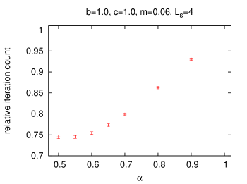
Figure 1: Relative iteration count $n_{i}(\alpha)/n_{i}(\alpha=1)$ for 3 gauge fields of size $16^{3}\times 32$.

Figure 2: Relative iteration count $n_{i}(\alpha)/n_{i}(\alpha=1)$ for 3 gauge fields of size $16^{3}\times 32$.

Figure 3: Relative iteration count $n_{i}(\alpha)/n_{i}(\alpha=1)$ for 3 gauge fields of size $16^{3}\times 32$.

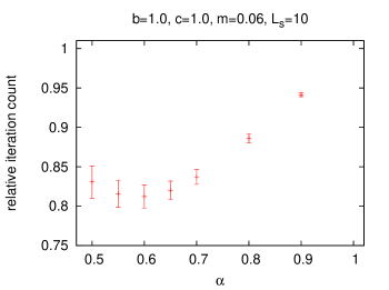
Figure 4: Relative iteration count $n_{i}(\alpha)/n_{i}(\alpha=1)$ for 3 gauge fields of size $16^{3}\times 32$.

Figure 5: Relative iteration count $n_{i}(\alpha)/n_{i}(\alpha=1)$ for 3 gauge fields of size $16^{3}\times 32$.

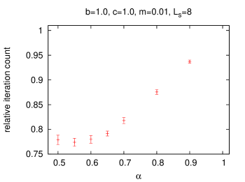
Figure 6: Relative iteration count $n_{i}(\alpha)/n_{i}(\alpha=1)$ for 3 gauge fields of size $16^{3}\times 32$.

Figure 7: Relative iteration count $n_{i}(\alpha)/n_{i}(\alpha=1)$ for 3 gauge fields of size $16^{3}\times 32$.

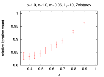
Figure 8: Relative iteration count $n_{i}(\alpha)/n_{i}(\alpha=1)$ for 3 gauge fields of size $16^{3}\times 32$, with $b_{i}=c_{i}$.

Appendix A Domain Wall to Overlap transformation

To keep notation simple, we perform the transformation with $L_{s}=4$ sites in the 5th dimension. A generalisation to arbitrary $L_{s}$ is straightforward.

The Domain Wall to Overlap transformation reads,

$$LD_{DW}(m)R=FD^{5}_{OV}(m).$$ (32)

The transformation matrices take the form (for $L_{s}$ sites in the 5th dimension),

$$F=LD_{DW}(1)R,$$ (33)

and

$$L\hskip-1.42271pt=\hskip-1.42271ptL_{1}L_{2}\hskip-1.42271pt=\hskip-1.42271pt\left[\begin{array}[]{cccc}1&S_{1}&S_{1}S_{2}&S_{1}S_{2}S_{3}\\ 0&1&S_{2}&S_{2}S_{3}\\ 0&0&1&S_{3}\\ 0&0&0&1\end{array}\right]\hskip-2.84544pt\left[\begin{array}[]{cccc}Q_{1-}^{-1}&0&0&0\\ 0&Q_{2-}^{-1}&0&0\\ 0&0&Q_{3-}^{-1}&0\\ 0&0&0&Q_{4-}^{-1}\\ \end{array}\right]\gamma_{5},$$ (42)

$$R=PR_{1}=\left[\begin{array}[]{cccc}P_{-}&P_{+}&0&0\\ 0&P_{-}&P_{+}&0\\ 0&0&P_{-}&P_{+}\\ P_{+}&0&0&P_{-}\\ \end{array}\right]\left[\begin{array}[]{cccc}-1&0&0&0\\ -S_{2}S_{3}S_{4}\,c_{+}&1&0&0\\ -S_{3}S_{4}\,c_{+}&0&1&0\\ -S_{4}\,c_{+}&0&0&1\\ \end{array}\right],$$ (51)

$$D^{5}_{OV}(m)=\left[\begin{array}[]{cccc}D^{4}_{OV}(m)&0&0&0\\ 0&1&0&0\\ 0&0&1&0\\ 0&0&0&1\\ \end{array}\right].$$ (56)

The matrix entries are defined as follows,

$$Q_{i+}=\gamma_{5}D_{w}(b_{i}P_{+}+c_{i}P_{-})+1,\;\;\;Q_{i-}=\gamma_{5}D_{w}(b_{i}P_{-}+c_{i}P_{+})-1,$$

$$S_{i}=T_{i}^{-1}=-Q_{i-}^{-1}Q_{i+},$$

$$c_{+}=P_{+}-mP_{-},\;\;\;c_{-}=P_{-}-mP_{+}.$$ (57)

$T_{i}^{-1}$ is called the transfer matrix.

The matrix multiplications will be performed in the following order,

$$L_{1}L_{2}D_{DW}(m)PR_{1}=L_{1}L_{2}M_{1}R_{1}=L_{1}M_{2}R_{1}=L_{1}M_{3}=M_{4}.$$ (58)

Step 1:

$$M_{1}=D_{DW}(m)P=\gamma_{5}\left[\begin{array}[]{cccc}Q_{1-}c_{-}&Q_{1+}&0&0\\ 0&Q_{2-}&Q_{2+}&0\\ 0&0&Q_{3-}&Q_{3+}\\ Q_{4+}c_{+}&0&0&Q_{4-}\\ \end{array}\right],$$ (63)

with

$$Q_{i-} = \gamma_{5}(D_{i+}P_{-}+D_{i-}P_{+})$$ (64)

$$= \gamma_{5}(D_{w}(b_{i}P_{-}+c_{i}P_{+})+P_{-}-P_{+})$$

$$= \gamma_{5}D_{w}(b_{i}P_{-}+c_{i}P_{+})-1,$$

$$Q_{i+} = \gamma_{5}(D_{i+}P_{+}+D_{i-}P_{-})$$ (65)

$$= \gamma_{5}(D_{w}(b_{i}P_{+}+c_{i}P_{-})+P_{+}-P_{-})$$

$$= \gamma_{5}D_{w}(b_{i}P_{+}+c_{i}P_{-})+1.$$

Step 2:

$$M_{2}=L_{2}M_{1}=\left[\begin{array}[]{cccc}c_{-}&-S_{1}&0&0\\ 0&1&-S_{2}&0\\ 0&0&1&-S_{3}\\ -S_{4}c_{+}&0&0&1\\ \end{array}\right].$$ (70)

Step 3:

$$M_{3}=M_{2}R_{1}=\left[\begin{array}[]{cccc}-c_{-}+S_{1}S_{2}S_{3}S_{4}c_{+}&-S_{1}&0&0\\ 0&1&-S_{2}&0\\ 0&0&1&-S_{3}\\ 0&0&0&1\\ \end{array}\right].$$ (75)

Step 4:

$$LD_{DW}(m)R=M_{4}=L_{1}M_{3}=\left[\begin{array}[]{cccc}-c_{-}+S_{1}S_{2}S_{3}S_{4}c_{+}&0&0&0\\ 0&1&0&0\\ 0&0&1&0\\ 0&0&0&1\\ \end{array}\right].$$ (80)

This leads to,

$$F=LD_{DW}(1)R=\left[\begin{array}[]{cccc}(1+S_{1}S_{2}S_{3}S_{4})\gamma_{5}&0&0&0\\ 0&1&0&0\\ 0&0&1&0\\ 0&0&0&1\\ \end{array}\right].$$ (85)

To make notation simpler, we define $S=S_{1}S_{2}S_{3}S_{4}$. The 5D Overlap Operator takes the form,

$$D^{5}_{OV}(m)=F^{-1}M_{4}=\left[\begin{array}[]{cccc}\gamma_{5}(1+S)^{-1}(-c_{-}+Sc_{+})&0&0&0\\ 0&1&0&0\\ 0&0&1&0\\ 0&0&0&1\\ \end{array}\right].$$ (90)

It follows for the $(11)$ element,

$$D^{5}_{OV}(m)_{11} = \frac{1}{2}\gamma_{5}(1+S)^{-1}\left(m+m\gamma_{5}-1+\gamma_{5}+S(1+\gamma_{5}-m+m\gamma_{5})\right)$$ (91)

$$= \frac{1}{2}\gamma_{5}(1+S)^{-1}\left((1+m)(S+1)\gamma_{5}+(1-m)(S-1)\right)$$

$$= \frac{1}{2}\left((1+m)+(1-m)\gamma_{5}\frac{(S-1)}{(S+1)}\right).$$

Hence eq.(90) takes the form,

$$D^{5}_{OV}(m)=\left[\begin{array}[]{cccc}\frac{1}{2}\left((1+m)+(1-m)\gamma_{5}\frac{(S-1)}{(S+1)}\right)&0&0&0\\ 0&1&0&0\\ 0&0&1&0\\ 0&0&0&1\\ \end{array}\right].$$ (96)

The matrix that acts as the variable for the polar decomposition can be found by setting,

$$\frac{(S-1)}{(S+1)}=\frac{(1-1/S)}{(1+1/S)}=\frac{\Pi_{i=1}^{4}(1+a_{i}X_{i})-\Pi_{i=1}^{4}(1-a_{i}X_{i})}{\Pi_{i=1}^{4}(1+a_{i}X_{i})+\Pi_{i=1}^{4}(1-a_{i}X_{i})},$$ (97)

and therefore

$$\frac{1}{S}=\frac{1}{S_{1}S_{2}S_{3}S_{4}}=\frac{(1-a_{1}X_{1}(1-a_{2}X_{2})(1-a_{3}X_{3})(1-a_{4}X_{4})}{(1+a_{1}X_{1})(1+a_{2}X_{2})(1+a_{3}X_{3})(1+a_{4}X_{4})}.$$ (98)

For each $i$, we determine $X_{i}$,

$$S_{i}^{-1}=(1-a_{i}X_{i})(1+a_{i}X_{i})^{-1}$$

$$Q_{i-}^{-1}Q_{i+}=(a_{i}X_{i}+1)(a_{i}X_{i}-1)^{-1}$$

$$Q_{i+}(a_{i}X_{i}-1)=Q_{i-}(a_{i}X_{i}+1)$$

$$a(Q_{i+}-Q_{i-})X_{i}=Q_{i+}+Q_{i-}$$

$$a_{i}\gamma_{5}((b_{i}-c_{i})D_{w}+2)\gamma_{5}X_{i}=(b_{i}+c_{i})\gamma_{5}D_{w}.$$ (99)

This results in,

$$a_{i}X_{i}=(b_{i}+c_{i})\gamma_{5}D_{w}\frac{1}{2+(b_{i}-c_{i})D}.$$ (100)

We can therefore write,

$$D^{5}_{OV}(m)=\left[\begin{array}[]{cccc}D^{4}_{OV}(m)&0&0&0\\ 0&1&0&0\\ 0&0&1&0\\ 0&0&0&1\\ \end{array}\right].$$ (105)

Appendix B Computation of the 4D propagator

It follows directly from,

$$\left[\begin{array}[]{cccc}D_{OV}^{4}&0&0&0\\ 0&1&0&0\\ 0&0&1&0\\ 0&0&0&1\\ \end{array}\right]\left(\begin{array}[]{c}x_{1}\\ x_{2}\\ x_{3}\\ x_{4}\end{array}\right)=\left(\begin{array}[]{c}b_{1}\\ b_{2}\\ b_{3}\\ b_{4}\end{array}\right),$$ (118)

or

$$D_{OV}^{4}x_{1}=b_{1},$$ (119)

that the 4D propagator is equal to $x_{1}$. We use eq.(32) and find

$$F^{-1}LD_{DW}(m)R\vec{x}=\vec{b},$$ (120)

or

$$R_{1}^{-1}(1)P^{-1}D_{DW}^{-1}(1)D_{DW}(m)PR_{1}\vec{x}=\vec{b}.$$ (121)

It follows from

$$R_{1}(1)D^{5}_{OV}R_{1}^{-1}\vec{y}=\left[\begin{array}[]{cccc}D^{4}_{OV}&0&0&0\\ S_{2}S_{3}S_{4}(\gamma_{5}D^{4}_{OV}-c_{+})&1&0&0\\ S_{3}S_{4}(\gamma_{5}D^{4}_{OV}-c_{+})&0&1&0\\ S_{4}(\gamma_{5}D^{4}_{OV}-c_{+})&0&0&1\\ \end{array}\right]\vec{y}=\vec{b},$$ (126)

that $y_{1}=x_{1}$, i.e. that the 4D propagator is not affected by the transformation with $R_{1}$. Hence we can use

$$P^{-1}D_{DW}^{-1}(1)D_{DW}(m)P\vec{y}=\vec{b},$$ (127)

or

$$D_{DW}(m)P\vec{y}=D_{DW}(1)P\vec{b},$$ (128)

to determine the 4D propagator $y_{1}$.