Drag of ballistic electrons by an ion beam

Abstract

Drag of electrons of 1D ballistic nanowire by a nearby 1D beam of ions is considered. We assume that the ion beam is represented by an ensemble of heavy ions of the same velocity $\bf V$. The ratio of the drag current to primary current carried by the ion beam is calculated.

The drag current appears to be a nonmonotonic function of velocity $V$, it has maxima for $V$ near $v_{nF}/2$ where $n$ is the number of electron miniband (channel) and $v_{nF}$ is the corresponding Fermi velocity. This means that the ion beam drag can be applied for ballistic nanostructure spectroscopy.

I Formulation of the problem

Drag as a physical phenomenon in solids can be described as follows. Consider a solid with two types of quasiparticles (type 1 and type 2). One creates a flux of the quasiparticles of type 2, the so-called driving current. As a result of the interaction between particles a current of quasiparticles of type 1, the so-called drag current is excited. An example of such phenomenon is the Coulomb drag where a current in conductor creates a current in adjacent conductor — see papers by Pogrebinski Pog and Price Price .

The purpose of the present paper is to consider a somewhat different situation where the driving current is created by real particles outside the conductor (rather than by quasiparticles within it). This would provide a contactless method to generate a drag current (or voltage) in a nanostructure.

Two formulations of the problem are feasible.

1. The dragging flux consists of heavy ions of almost the same velocity $\bf V$.

2. One considers a flux of weakly ionized gas that is in thermal equilibrium having some temperature $T$ and hydrodynamical velocity $\bf V$.

In the present paper we treat the first possibility. In other words, we consider an ion beam, i. e. a flux of ions having the same velocity $\bf V$. For the simplest situation the value of velocity $\bf V$ is determined by the accelerating voltage $\mathfrak{V}$ and the ion mass $M$ as

$$\frac{MV^{2}}{2}=e_{I}\mathfrak{V}.$$ (1)

Here $e_{I}$ is the charge of an ion.

For the drag system we will treat a ballistic (collisionless) electron transport in a quantum wire. Such nanoscale systems may have rather low electron densities that can be varied by means of the gate voltage. The collisionless quantum wires act as waveguides for the electron de Broglie waves. For a strong Fermi degeneracy

$$T\ll\mu$$ (2)

where $T$ is the temperature (we will use the energy units for it) while $\mu$ is the Fermi energy, each miniband of transverse quantisation (channel) gives the following contribution to the conductance

$$G_{0}=\frac{e^{2}}{\pi\hbar},$$ (3)

($e$ being the electron charge) so that the total conductance is

$$G={\cal N}G_{0}.$$

Here ${\cal N}$ is the number of such active channels, i. e. the minibands with bottoms $\epsilon_{n}(0)$ below the Fermi level $\mu$.

Our purpose is to investigate the main features of this drag phenomenon. We assume that the distance $d$ between the ion beam and the wire is much larger than the width of the wire, so that on the scale of this width the Coulomb interaction of ions and electrons is a smooth function. Then the selection rules for the corresponding matrix elements require that electrons involved in the transitions change their quasimomenta but remain within the initial transverse quantized channel $n$. One can vary the velocity $\bf V$ of the ions with the accelerating voltage $\mathfrak{V}$ and measure the resulting variation of the drag current (or drag voltage). We will denote by ${\cal V}_{\bf r}$ the volume occupied by the nanowire while ${\cal V}_{\bf R}$ will be the volume where the flux of ions propagates and interacts with the electrons of the nanowire. We assume both ${\cal V}_{\bf r}$ and ${\cal V}_{\bf R}$ to have a 1D shape of length $L$ parallel to $z$-axis.

One can give the following qualitative considerations concerning the drag by an ion beam. Due to the conservation of such quantities as the energy, the transverse quantized channel number $n$ and the (quasi)momentum in the electron-ion collisions one has to consider in the Born approximation the transition of electron from $|n,p\rangle$ to $|n,p+q_{z}\rangle$ state (where $p$ is the $z$-component of electron quasimomentum) and that of the ion from $|{\bf P}\rangle$ to $|{\bf P}-{\bf q}\rangle$ state according to relation

$$\frac{p^{2}}{2m}+\frac{{\bf P}^{2}}{2M}=\frac{(p+q_{z})^{2}}{2m}+\frac{({\bf P}-{\bf q})^{2}}{2M}.$$ (4)

The $\delta$-function describing the energy conservation can be therefore written as

$$\delta\left[\frac{q_{z}^{2}}{2m}(1+m/M)+\frac{q_{z}}{m}(p-mV)+\frac{q_{\perp}^{2}}{2M}\right]\simeq\,\frac{2m}{|q_{z}|}\delta\left[q_{z}-2(mV-p)\right],$$ (5)

where $P_{z}\equiv P=MV$. Further on we will take into account that $m/M\,\ll\,1$ and neglect $m/M$ as compared to 1 and $(m/M)q_{\perp}^{2}$ as compared to $q_{z}^{2}$. Therefore the transferred (quasi)momentum is $q_{z}=2(mV-p)$ and the probability of such a transition includes the factor

$$f_{np}(1-f_{n,p+q_{z}})-f_{n,p+q_{z}}(1-f_{np})=f_{np}-f_{n,2mV-p}$$ (6)

as well as the electron-ion Coulomb interaction matrix element squared. For the 1D situation under consideration it has a factor proportional to

$$\left.K_{0}^{2}(|q_{z}|d/\hbar)\right|_{q_{z}=2(mV-p)}$$ (7)

where $d$ is the distance between the ion beam and the wire and $K_{0}$ is the McDonald function [see below Eq. (17)]. One can use for it the following approximate equations

$$K_{0}(s)\approx\ln\frac{2}{\gamma s}\quad\mbox{for}\quad s\ll 1,$$ (8)

$$K_{0}(s)\approx\sqrt{\frac{\pi}{2s}}e^{-s}\quad\mbox{for}\quad s\gg 1$$ (9)

where $\ln{\gamma}=0.5772$. The drag current is proportional to the sum over electron momenta $p$ of the products in Eqs. (5) — (7). We consider $p<0$ and require the state $p$ to be occupied, this condition leads to $-p_{F}<p<0$. The requirement that the final state with momentum $2mV-p$ should be empty gives $2mV-p>p_{F}$ provided $V<v_{F}/2$ (see Fig. 1). If $V>v_{F}/2$ there is no additional restriction except $-p_{F}<p<0$, i.e. all occupied states are involved in transitions.

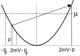
Figure 1: Momenta from $-p_{F}$ to $2mV-p_{F}$ are involved in transitions. If $V>v_{F}/2$ all negative momenta $p$ contribute to the drag current.

Therefore, if $V<v_{F}/2$ we get for the drag current

$$J_{d}\propto\,\int_{-p_{F}}^{-p_{F}+2mV}dp\frac{K_{0}^{2}[2(mV-p)d/\hbar]}{mV-p}=\int_{p_{F}-mV}^{p_{F}+mV}dp\frac{K_{0}^{2}(2pd/\hbar)}{p}$$ (10)

and we see that increase in $V$ decreases the minimal transferred momentum and increases the effective Coulomb interaction $K_{0}(2pd/\hbar)$. If $V>v_{F}/2$ we have

$$J_{d}\propto\,\int_{-p_{F}}^{0}dp\frac{K_{0}^{2}\left[2(mV-p)d/\hbar\right]}{mV-p}=\int_{mV}^{p_{F}+mV}dp\frac{K_{0}^{2}(2pd/\hbar)}{p}$$ (11)

and increase of $V$ results in a decrease of the drag current. These equations provide an adequate description of the drag current dependence on the ion beam velocity as can be readily seen in our quantitative approach below.

II Interaction of ion beam with electrons of nanostructure

For simplicity, we assume the width of the beam to be constant (actually it may slightly vary in the course of beam propagation). Then one can write the distribution of the ions within the beam as

$$F_{\bf P}=N(2\pi\hbar)^{3}\delta(P_{x})\delta(P_{y})\delta(P_{z}-P),$$ (12)

$N$ being the ion concentration.

The collision term of the Boltzmann equation for 1D electrons and 3D ions is in the Born approximation

$$\left[\frac{{\partial f}_{pn}}{\partial t}\right]_{\rm coll}\equiv I\{f,F\}=\int\frac{{\cal V}_{\bf R}d^{3}P}{(2\pi\hbar)^{3}}\int\frac{{\cal V}_{\bf R}d^{3}q}{(2\pi\hbar)^{3}}\frac{2\pi}{\hbar}\left|\langle{p,n},{\bf P}|U|{{p+q_{z},n},{\bf P-q}}\rangle\right|^{2}$$

$$\times\delta(\epsilon_{n{p}}+E_{\bf P}-\epsilon_{n,{p+q_{z}}}-E_{\bf P-q})\left[f_{n{p}}(1-f_{n,{p+q_{z}}})F_{\bf P}-f_{np+q_{z}}(1-f_{np})F_{{\bf P}-{\bf q}}\right]$$ (13)

where

$$\epsilon_{n}(p)=\epsilon_{n}(0)+p^{2}/2m$$ (14)

Here $n$ is the number of the channel, i.e. of the mini-band of 1D transverse quantization (according to the assumption made above this number does not change in the course of electron transitions), $\bf q$ is the transferred (quasi)momentum, $M$ is the mass of an ion, $m$ is the effective mass of conduction electron and

$$U=\frac{2}{1+\kappa}\frac{ee_{I}}{|{\bf R-r}|}$$ (15)

describes the Coulomb interaction of the ion with charge $e_{I}$ and electron in the wire, $\kappa$ being the dielectric susceptibility of the wire. For the matrix element in Eq.(13) we have

$$\langle{p,n,{\bf P}}|U|p+q_{z},n,{\bf P}-{\bf q}\rangle=\int_{\cal V_{\bf r}}d^{3}r\int_{\cal V_{\bf R}}d^{3}R\psi^{\ast}_{n}({\bf r}_{\perp})\Psi^{*}_{\bf P}\frac{2ee_{I}}{L(1+\kappa)|{\bf r-R}|}\psi_{n}({\bf r}_{\perp})\Psi_{{\bf P-q}}e^{iq_{z}z/\hbar}.$$ (16)

Since

$$\int\frac{dZdz}{L|{\bf r-R}|}e^{iq_{z}(z-Z)/\hbar}=2K_{0}(|q_{z}||{\Delta{\bf r_{\perp}}}|/\hbar)$$ (17)

where

$$|\Delta{\bf r_{\perp}}|\equiv\sqrt{(x-X)^{2}+(y-Y)^{2}}$$

we can write

$$\langle{p,n,{\bf P}}|U|p+q_{z},n,{\bf P}-{\bf q}\rangle=$$

$$\frac{4ee_{I}}{(1+\kappa){\cal V}_{\bf R}}\int d{\bf R}_{\perp}\int d{\bf r}_{\perp}|\psi_{n}({\bf r}_{\perp})|^{2}{e^{-i{\bf q}_{\perp}{\bf R}_{\perp}/\hbar}}K_{0}(|q_{z}||\Delta{\bf r}_{\perp}|/\hbar).$$ (18)

The Boltzmann equation for electrons is

$$v\frac{\partial f_{np}}{\partial z}=-\left[\frac{{\partial f}_{np}}{\partial t}\right]_{\rm coll},$$ (19)

where

$$v=\frac{d\epsilon_{pn}}{dp}=\frac{p}{m}$$

is the electron velocity.

To calculate the current in the wire, we iterate the Boltzmann equation for the electrons of the wire in the term describing collisions between electrons of the wire and ions. In the zeroth approximation one can choose the electron distribution function in the collision term to be equilibrium one. In what follows $f_{np}\equiv\,f_{F}(\epsilon_{np}-\mu)$ will be implied, where $f_{F}$ is the Fermi distribution function while $\mu$ is the Fermi level. The first iteration of Eq.(19) gives for the nonequilibrium part of the distribution function

$$\Delta f_{n{p}}=-\left(z\pm\frac{L}{2}\right)\frac{1}{v_{np}}I\{f,F\}$$ (20)

for $p>0$ and $p<0$, respectively. Here $I\{f,F\}$ is a shorthand notation for the collision term. Using the particle conservation property of the scattering integral

$$\sum_{n}\int dpI\{f,F\}=0$$ (21)

we get for the drag current $J_{d}$ (cf. with Ref. GM1, )

$$J_{d}=-2eL\sum_{n}\int_{0}^{\infty}\frac{dp}{2\pi\hbar}I\{f,F\}.$$ (22)

With the distribution function given by Eq.(12) we have

$$J_{d}=-2eN{\cal V}_{\bf R}^{2}L\sum_{n}\int_{0}^{\infty}\frac{dp}{2\pi\hbar}\int\frac{d^{3}q}{(2\pi\hbar)^{3}}\frac{2\pi}{\hbar}\left\{\left|\langle{p,n},P{\bf e}_{z}|U|{{p+q_{z},n},P{\bf e}_{z}-{\bf q}}\rangle\right|^{2}\right.$$ (23)

$$\times\delta(\epsilon_{n{p}}+E_{P{\bf e}_{z}}-\epsilon_{n,{p+q_{z}}}-E_{P{\bf e}_{z}-{\bf q}})f_{n{p}}(1-f_{n,{p+q_{z}}})-$$

$$-\left|\langle{p,n},P{\bf e}_{z}+{\bf q}|U|{{p+q_{z},n},P{\bf e}_{z}}\rangle\right|^{2}\left.\delta(\epsilon_{n{p}}+E_{P{\bf e}_{z}+{\bf q}}-\epsilon_{n,{p+q_{z}}}-E_{P{\bf e}_{z}})f_{n{p+q_{z}}}(1-f_{n,{p}})\right\}$$

where ${\bf e}_{z}$ is the unit vector along the $z$ axis. In the first term under the integral we change ${\bf q}\rightarrow\,-{\bf q}$ and shift the integration variable $p$ by $q_{z}$, then

$$J_{d}=-2eN{\cal V}_{\bf R}^{2}L\sum_{n}\int\frac{d^{3}q}{(2\pi\hbar)^{3}}\int_{0}^{q_{z}}\frac{dp}{2\pi\hbar}\frac{2\pi}{\hbar}\left|\langle{p,n,P{\bf e}_{z}+{\bf q}}|U|p+q_{z},n,P{\bf e}_{z}\rangle\right|^{2}$$ (24)

$$\times\delta(\epsilon_{n{p}}+E_{P{\bf e}_{z}+{\bf q}}-\epsilon_{n,{p-q_{z}}}-E_{P{\bf e}_{z}})f_{n{p-q_{z}}}(1-f_{n,{p}}),$$

so that the drag current is

$$J_{d}=-J_{0}\frac{2MS_{\bf R}}{m\pi^{2}\hbar^{2}}\sum_{n}\int dq_{z}\int_{0}^{q_{z}}dpf_{n{p-q_{z}}}(1-f_{n,{p}})\int d{\bf q}_{\perp}g({\bf q}_{\perp},|q_{z}|)$$

$$\times\delta\left[q_{\perp}^{2}-q_{z}^{2}(M/m-1)+2q_{z}(Mp/m+P)\right].$$

Here we introduced

$$J_{0}=\frac{e(2ee_{I})^{2}LNmS_{\bf R}}{(1+\kappa)^{2}\pi\hbar^{3}}$$

and a dimensionless quantity $g({\bf q}_{\perp},|q_{z}|)$ according to

$$S_{\bf R}^{2}g({\bf q}_{\perp},|q_{z}|)=\left|\int d{\bf R}_{\perp}d{\bf r}_{\perp}{e^{-i{\bf q}_{\perp}{\bf R}_{\perp}/\hbar}}|\psi_{n}({\bf r}_{\perp})|^{2}K_{0}(|q_{z}||\Delta{\bf r}_{\perp}|/\hbar)\right|^{2}$$ (25)

where $S_{\bf R}$ is the cross section area of the ion beam.

We get

$$J_{d}=J_{0}\frac{2MS_{\bf R}}{m\pi^{2}\hbar^{2}}\sum_{n}\int_{0}^{\infty}dq_{z}\int_{0}^{q_{z}}dpf_{n{p-q_{z}}}(1-f_{n,{p}})\int d{\bf q}_{\perp}g({\bf q}_{\perp},q_{z})$$

$$\times\left\{\delta\left[q_{\perp}^{2}-q_{z}^{2}(M/m-1)+2q_{z}(Mp/m-P)\right]\right.$$

$$\left.-\delta\left[q_{\perp}^{2}-q_{z}^{2}(M/m-1)+2q_{z}(Mp/m+P)\right]\right\}.$$ (26)

II.1 Linear response

In the linear response regime

$$V\,\ll\,T/p_{nF}\quad\mbox{where}\quad p_{nF}=\sqrt{2m[\mu-\epsilon_{n}(0)]}$$ (27)

the difference of $\delta$-functions in Eq.(26) can be expanded as (we again take into account that $M/m\,\gg\,1$)

$$\delta\left[q_{\perp}^{2}-q_{z}^{2}M/m+2q_{z}(Mp/m+P)\right]-\delta\left[q_{\perp}^{2}-q_{z}^{2}M/m+2q_{z}(Mp/m-P)\right]$$

$$=\frac{m}{2M|q_{z}|}\left\{\delta\left[mq_{\perp}^{2}/2Mq_{z}-q_{z}/2+p+mV\right]-\delta\left[mq_{\perp}^{2}/2Mq_{z}-q_{z}/2+p-mV\right]\right\}$$

$$=mV\frac{m}{M|q_{z}|}\frac{\partial}{\partial p}\delta\left[mq_{\perp}^{2}/2Mq_{z}-q_{z}/2+p\right].$$

Then integration by parts gives

$$J_{d}=J_{0}\frac{2S_{\bf R}}{\pi^{2}\hbar^{2}}mV\sum_{n}\int_{0}^{\infty}\frac{dq_{z}}{q_{z}}\int_{0}^{q_{z}}dp\int d{\bf q}_{\perp}g({\bf q}_{\perp},q_{z})$$

$$\times\delta\left[mq_{\perp}^{2}/2Mq_{z}-q_{z}/2+p\right]\frac{\partial}{\partial p}f_{n{p-q_{z}}}(1-f_{n,{p}}).$$ (28)

Using

$$\frac{\partial}{\partial p}f_{n{p-q_{z}}}(1-f_{n,{p}})=(1-f_{n,{p}})\delta(q_{z}-p-p_{nF})+f_{n{p-q_{z}}}\delta(p-p_{nF})$$ (29)

we have

$$J_{d}=J_{0}\frac{4S_{\bf R}}{\pi^{2}\hbar^{2}}mV\sum_{n}\int_{p_{nF}}^{\infty}dq_{z}\int d{\bf q}_{\perp}g({\bf q}_{\perp},q_{z})$$

$$\times\left\{\delta\left[q^{2}_{z}-2p_{nF}q_{z}+mq_{\perp}^{2}/M\right](1-f_{n,q_{z}-p_{nF}})+\delta\left[q^{2}_{z}-2p_{nF}q_{z}-mq_{\perp}^{2}/M\right]f_{n,p_{nF}-q_{z}}\right\}.$$ (30)

Eliminating the $\delta$-functions we get

$$J_{d}=J_{0}\frac{2S_{\bf R}}{\pi^{2}\hbar^{2}}mV\sum_{n}\int d{\bf q}_{\perp}\left\{g({\bf q}_{\perp},p_{nF}+p_{1})\frac{(1-f_{n,p_{1}})}{p_{1}}+g({\bf q}_{\perp},p_{nF}+p_{2})\frac{f_{n,p_{2}}}{p_{2}}\right\},$$

where $p_{1}=\sqrt{p_{nF}^{2}-mq_{\perp}^{2}/M}$ and $p_{2}=\sqrt{p_{nF}^{2}+mq_{\perp}^{2}/M}$. The expression for $J_{d}$ can be simplified as follows

$$J_{d}=J_{0}\frac{4S_{\bf R}}{\pi^{2}\hbar^{2}}mV\sum_{n}\frac{1}{p_{nF}}\int d{\bf q}_{\perp}\frac{g({\bf q}_{\perp},2p_{nF})}{e^{q_{\perp}^{2}/2MT}+1}.$$ (31)

If the ion beam cross section is of a circular form with radius $a$ we have

$$g({\bf q}_{\perp},2p_{nF})=\left(\frac{2\hbar J_{1}(aq_{\perp}/\hbar)}{aq_{\perp}}\right)^{2}K_{0}^{2}(2p_{nF}d/\hbar),$$ (32)

where $J_{1}(x)$ is the Bessel function of the first order and $d$ is the distance between the ion flux and the wire.

Below we will discuss in more detail a special case where $g({\bf q}_{\perp},2p_{nF})$ does not depend on ${\bf q}_{\perp}$. For instance, this is the case provided

$$\sqrt{MT}\,\ll\,\hbar/a.$$ (33)

Then for ${\cal N}=1$ we get

$$J_{d}=J_{0}\frac{4\ln{(4)}a^{2}}{\hbar^{2}}(MT)\frac{V}{v_{F}}K_{0}^{2}(2p_{F}d/\hbar),$$ (34)

where $v_{F}=p_{F}/m$ is the Fermi velocity and

$$J_{0}=\frac{e(2ee_{I})^{2}LNma^{2}}{(1+\kappa)^{2}\hbar^{3}}.$$ (35)

For the opposite case where

$$\sqrt{MT}\,\gg\,\hbar/a$$ (36)

the drag does not depend on temperature. For the values $M=10^{-22}$g (Ga), $T=4$K, $a=10^{-5}$cm this inequality can be easily satisfied. Then we have

$$J_{d}=J_{0}\frac{8V}{v_{F}}K_{0}^{2}\left(\frac{2p_{F}d}{\hbar}\right).$$ (37)

It is interesting to calculate the ratio $J_{d}/J_{I}$ for this case

$$\frac{J_{d}}{J_{I}}=\frac{e}{e_{I}}\frac{32(ee_{I})^{2}Lm}{(1+\kappa)^{2}\pi\hbar^{3}v_{F}}K_{0}^{2}\left(\frac{2p_{F}d}{\hbar}\right).$$ (38)

Here one can use for $K_{0}(s)$ equations (8) and (9).

For an estimate we assume the following values $L=10^{-4}$cm, $m=7\cdot 10^{-29}$g, $v_{F}=2\cdot 10^{7}$cm/s, $\kappa=10$, $p_{F}d/\hbar=2$, so that $K_{0}^{2}(2p_{F}d/\hbar)=1.3\cdot 10^{-4}$. Then for $J_{I}=10^{-8}$A one gets $J_{d}=2\cdot 10^{-9}$A and the corresponding drag voltage ${\cal V}_{d}$ is about

$${\cal V}_{d}=20\,\,\mu\mbox{V}.$$ (39)

Naturally, if $J_{I}$ goes up ${\cal V}_{d}$ also goes up in proportion to $J_{I}$.

II.2 Nonlinear case

We consider the simplest case of low temperatures assuming that

$$V\,\gg\,T/p_{F}.$$ (40)

In our further calculation we will assume $T=0$, then the integration due to the Fermi functions in Eq.(26) is restricted and we get (the first or the second $\delta$-function contributes for $V>0$ and $V<0$ respectively, so that the drag current changes its sign with $V$ as it should)

$$J_{d}=J_{0}\frac{a^{2}}{\pi\hbar^{2}}\sum_{n}\left(\int_{p_{nF}}^{2p_{nF}}\frac{dq_{z}}{q_{z}}\int_{p_{nF}}^{q_{z}}dp+\int_{2p_{nF}}^{\infty}\frac{dq_{z}}{q_{z}}\int_{q_{z}-p_{nF}}^{q_{z}}dp\right)$$

$$\times\int d{\bf q}_{\perp}g({\bf q}_{\perp},q_{z})\delta\left[p-mV-q_{z}(1-m/M)/2+mq_{\perp}^{2}/2q_{z}M\right].$$

The result valid for

$$V<v_{F}/2$$ (41)

is

$$J_{d}=J_{0}\frac{a^{2}}{\pi\hbar^{2}}\sum_{n}\int d{\bf q}_{\perp}\Theta[4Pp_{nF}-q_{\perp}^{2}]\int_{p_{-}}^{p_{+}}\,\frac{dq_{z}}{q_{z}}g({\bf q}_{\perp},q_{z})$$ (42)

where $\Theta$ is the step function and

$$p_{\pm}=p_{nF}\pm mV+\sqrt{(p_{nF}\pm mV)^{2}\mp mq_{\perp}^{2}/M}$$

(other cases are considered in Appendix A).

For $V\ll\,v_{nF}$ the integration variable $q_{z}$ is in the vicinity of $2p_{nF}$ and we have

$$J_{d}=J_{0}\frac{a^{2}}{2\pi\hbar^{2}}\sum_{n}\int d{\bf q}_{\perp}\Theta[4Pp_{nF}-q_{\perp}^{2}]\left(4\frac{mV}{p_{nF}}-\frac{m}{M}\frac{q_{\perp}^{2}}{p_{nF}^{2}}\right)g({\bf q}_{\perp},2p_{nF}).$$ (43)

Eq.(43) substantially simplifies provided $g({\bf q}_{\perp},2p_{nF})$ does not depend on ${\bf q}_{\perp}$; this is the case provided the ion flux cross section characteristic width $a$ obeys the inequality

$$\sqrt{Pp_{nF}}a/\hbar\,\ll\,1.$$ (44)

Then

$$J_{d}=J_{1}\sum_{n}g(2p_{nF}),$$ (45)

where

$$J_{1}=J_{0}\frac{(2mV)^{2}a^{2}}{2\hbar^{2}}\frac{M}{m}.$$ (46)

This expression is valid for $V\,>\,0$, i.e. when the ion flux is directed ”to the right”. Then the momentum transferred to the electron system in the wire is also directed to the right and the current (since $e\,<\,0$) flows in the opposite direction regardless of the sign of dragging ion charge.

Assuming that the distance $d$ between the ion flux and the wire is much bigger than the characteristic cross section length of the wire and the flux we can write

$$g({\bf q}_{\perp},2p_{nF})\simeq\,K_{0}^{2}(2p_{nF}d/\hbar),$$ (47)

and

$$J_{d}=J_{1}\sum_{n}K_{0}^{2}(2p_{nF}d/\hbar).$$ (48)

Using for the function $K_{0}$ the approximate equation (9) we get

$$J_{d}=J_{1}\sum_{n}\frac{1}{k_{nF}d}e^{-4k_{nF}d},$$ (49)

where $k_{nF}=p_{nF}/\hbar$.

In the case $a\sqrt{Pp_{nF}}/\hbar\,\gg\,1$ the drag current is linear in $V$

$$J_{d}=4J_{0}MV\sum_{n}\frac{1}{p_{nF}}K_{0}^{2}(2p_{nF}d/\hbar).$$ (50)

Figure 2: Drag current dependence on the velocity of the ion beam. We take $v_{F}^{(2)}=kv_{F}^{(1)}$ and $k=3/2$. The first peak corresponds to $V/v_{F}^{(2)}=1/2k$ (i.e. $V/v_{F}^{(1)}=1/2$) and the second peak corresponds to $V/v_{F}^{(2)}=1/2$. Here $J_{0}=e(2ee_{I})^{2}LNma^{2}/(1+\kappa)^{2}\hbar^{3}$.

III Conclusive remarks

We have developed a theory of Coulomb drag of electrons in 1D ballistic nanostructure by an ion beam. This provides an example of drag of quasiparticles of the nanostructure by particles of the beam. It is worthwhile to mention that such a beam may consist not only of heavy ions but also of electrons. The free electron mass is usually bigger than the effective mass of conduction electrons, so that the adopted approximations of our calculation, $M\gg m$, may remain valid in this case too.

The experimental setup should permit one to vary the velocity $V$ within rather wide limits. We see however that to achieve a large drag effect one should choose the value of $V$ near to $v_{Fn}/2$ (see Fig. 2). This means in particular that the ion beam drag may be a useful instrument for nanostructure spectroscopy: it may make it possible to measure with appropriate accuracy the Fermi velocities $v_{Fn}$ in each channel $n$.

Appendix A Evaluation of the drag current for various ratios of $\alpha=V/v_{F}$

We introduce dimensionless parameters

$$\alpha=mV/p_{nF}=V/v_{nF}$$

and

$$b=mq_{\perp}^{2}/p_{nF}^{2}M$$

and write $q$ instead of $q(1-m/M)$ in the argument of the $\delta$-function

$$J_{d}=J_{0}\sum_{n}\left(\frac{p_{nF}a}{\hbar}\right)^{2}\frac{1}{\pi}\left(\int_{1}^{2}dq\int_{1}^{q}dp+\int_{2}^{\infty}dq\int_{q-1}^{q}dp\right)$$ (51)

$$\times\frac{1}{q}\int d{\bf q}_{\perp}g(p_{nF}{\bf q}_{\perp},p_{nF}q)\delta\left[p-\alpha-q/2+b/2q\right]$$

where

$$J_{0}=e(2ee_{I})^{2}LNma^{2}/(1+\kappa)^{2}\hbar^{3}.$$

For $\alpha<1/2$ we get

$$J_{d}=J_{0}\sum_{n}\left(\frac{p_{nF}a}{\hbar}\right)^{2}\frac{1}{\pi}\int d{\bf q}_{\perp}\Theta[4\alpha-b]\int_{A_{+}(-\alpha,-b)}^{A_{+}(\alpha,b)}dq\frac{g(p_{nF}{\bf q}_{\perp},p_{nF}q)}{q}$$ (52)

where $A_{\pm}(\alpha,b)=1+\alpha\pm\,\sqrt{(1+\alpha)^{2}-b}$.

If $1/2<\alpha<1$ we get

$$J_{d}=J_{0}\sum_{n}\left(\frac{p_{nF}a}{\hbar}\right)^{2}\frac{1}{\pi}\int d{\bf q}_{\perp}\left\{\Theta[2\alpha-1-b]\int_{A_{+}(\alpha-1,b)}^{A_{+}(\alpha,b)}dq\right.$$ (53)

$$\left.+\Theta[b-2\alpha+1]\Theta[4\alpha-b]\int_{A_{+}(-\alpha,-b)}^{A_{+}(\alpha,b)}dq\right\}\frac{g(p_{nF}{\bf q}_{\perp},p_{nF}q)}{q}.$$

We will not give here explicit expressions for larger values of $V/v_{F}$ but rather present the simple expression for the drag current valid for $\hbar/a\,\ll\,mV\sqrt{M/m}$

$$J_{d}=4J_{0}\int_{\alpha}^{\infty}\,dz\frac{K_{0}^{2}(2p_{F}zd/\hbar)}{z}\left(\frac{1}{e^{([z-\alpha]^{2}-1)p_{F}^{2}/2mT}+1}-\frac{1}{e^{([z+\alpha]^{2}-1)p_{F}^{2}/2mT}+1}\right).$$ (54)

This expression is reduced to Eq.(37) and Eq.(50) in the corresponding limiting cases. For $mV\,\gg\,T/v_{F}$ the difference of the Fermi functions restricts the integration region so that for $\alpha<1/2$ we have

$$J_{d}=4J_{0}\int_{1-\alpha}^{1+\alpha}\,dz\frac{K_{0}^{2}(2p_{F}zd/\hbar)}{z}$$ (55)

and

$$J_{d}=4J_{0}\int_{\alpha}^{1+\alpha}\,dz\frac{K_{0}^{2}(2p_{F}zd/\hbar)}{z}$$ (56)

for $\alpha>1/2$. The drag current calculated according to these simple formulas practically coincides with that calculated from the exact expressions and presented in Fig. 2 for the case ${\cal N}=2$.

Appendix B Preferred velocity of the beam

Let us differentiate Eq.(26) with respect to $mV$ and determine the sign of derivative. We get under the sign of integral the following sum of $\delta$-functions

$$-\frac{d}{dp}\left\{\delta\left[q_{\perp}^{2}m/M-q_{z}^{2}+2q_{z}(p-mV)\right]+\delta\left[q_{\perp}^{2}m/M-q_{z}^{2}+2q_{z}(p+mV)\right]\right\}.$$ (57)

We integrate over $p$ by parts and get (we denote the ratio $J_{d}\pi^{2}\hbar^{2}/(2J_{0}S_{\bf R}m)$ by $j$)

$$\frac{dj}{dV}=\int_{0}^{\infty}dq_{z}\int\,d{\bf q}_{\perp}g({\bf q}_{\perp},q_{z})\int_{0}^{q_{z}}dp\left\{\delta\left[q_{\perp}^{2}m/M-q_{z}^{2}+2q_{z}(p-mV)\right]\right.$$ (58)

$$+\left.\delta\left[q_{\perp}^{2}m/M-q_{z}^{2}+2q_{z}(p+mV)\right]\right\}\frac{d}{dp}\left[f_{n{p-q_{z}}}(1-f_{n,{p}})\right]$$

$$-\int_{0}^{\infty}dq_{z}\int\,d{\bf q}_{\perp}g({\bf q}_{\perp},q_{z})(1-f_{q_{z}})\left\{\delta\left[q_{\perp}^{2}m/M+q_{z}^{2}-2q_{z}mV\right]\right.$$

$$+\left.\delta\left[q_{\perp}^{2}m/M+q_{z}^{2}+2q_{z}mV\right]\right\}$$

We take into account the strong Fermi degeneracy of the electron system so that $1-f_{0}=0,\,f_{0}=1$. Using Eq.(29) we get

$$\frac{dj}{dV}=\int_{2p_{nF}}^{\infty}dq_{z}\int\,d{\bf q}_{\perp}g({\bf q}_{\perp},q_{z})\left\{\delta\left[q_{\perp}^{2}m/M+q_{z}^{2}-2q_{z}(p_{nF}+mV)\right]+\right.$$

$$\left.\delta\left[q_{\perp}^{2}m/M+q_{z}^{2}-2q_{z}(p_{nF}-mV)\right]\right\}$$

$$-\int_{p_{nF}}^{\infty}dq_{z}\int\,d{\bf q}_{\perp}g({\bf q}_{\perp},q_{z})\delta\left[q_{\perp}^{2}m/M+q_{z}^{2}-2q_{z}mV\right]$$ (59)

We again use $f_{q_{z}-p_{nF}}=1$ for $q_{z}>p_{nF}$ and take into account that $V>0$ so that the last $\delta$-function in Eq.(58) does not contribute. The second $\delta$-function in the first integral in the previous expression does not contribute as well and we arrive at

$$\frac{dj}{dV}=I_{+}-I_{-},$$

where we introduce notations for the positive and negative integrals

$$I_{+}=\int d{\bf q}_{\perp}\int_{2p_{nF}}^{\infty}dq_{z}g({\bf q}_{\perp},q_{z})\delta\left[q_{\perp}^{2}m/M+q_{z}^{2}-2q_{z}(p_{nF}+mV)\right]$$ (60)

$$I_{-}=\int d{\bf q}_{\perp}\int_{p_{nF}}^{\infty}dq_{z}g({\bf q}_{\perp},q_{z})\delta\left[q_{\perp}^{2}m/M+q_{z}^{2}-2q_{z}mV\right]$$ (61)

If $V/v_{nF}<1/2$ we get

$$I_{+}=\int_{q_{\perp}^{2}<4Mp_{nF}V}d{\bf q}_{\perp}\frac{g({\bf q}_{\perp},q_{1})}{2\sqrt{(p_{nF}+mV)^{2}-mq_{\perp}^{2}/M}}$$ (62)

where $q_{1}=p_{nF}+mV+\sqrt{(p_{nF}+mV)^{2}-mq_{\perp}^{2}/M}$ and $I_{-}=0$ and the drag current is an increasing function of the beam velocity $V$.

The integral $I_{-}$ has nonzero values only if $V/v_{nF}>1/2$. If $V/v_{nF}<1$ we have for this integral

$$I_{-}=\int_{q_{\perp}^{2}<Mp_{nF}(2mV-p_{nF})/m}d{\bf q}_{\perp}\frac{g({\bf q}_{\perp},q_{2})}{2\sqrt{(mV)^{2}-mq_{\perp}^{2}/M}}$$ (63)

where $q_{2}=mV+\sqrt{(mV)^{2}-mq_{\perp}^{2}/M}$. $I_{-}$ in this region becomes larger than $I_{+}$ (the latter being practically zero due to exponential dependence on $q_{1}$) and the drag current turns into decreasing function of the velocity $V$.

If $V/v_{nF}>1$

$$I_{-}=\int_{q_{\perp}^{2}<Mp_{nF}V}d{\bf q}_{\perp}\frac{g({\bf q}_{\perp},q_{2})}{2\sqrt{(mV)^{2}-mq_{\perp}^{2}/M}}$$ (64)

$$-\int_{q_{\perp}^{2}>Mp_{nF}(mV-p_{nF})/m}d{\bf q}_{\perp}\frac{g({\bf q}_{\perp},q_{3})}{2\sqrt{(mV)^{2}-mq_{\perp}^{2}/M}}$$ (65)

where $q_{3}=mV-\sqrt{(mV)^{2}-mq_{\perp}^{2}/M}$.

Therefore we see that the drag current has a maximum as a function of the beam velocity in the vicinity of $V=v_{nF}/2$.

References

(1)Pogrebinski M B 1977 Fiz. Tekh. Poluprov.11 637
(Engl. Transl. 1977 Sov. Phys.-Semicond. 11 372)
(2)Price P J 1983 Physica B 117 750
(3)Gurevich V L and Muradov M I 2000 Zh. Eksp. Teor. Fiz.
Pis’ma Red. 71, 164
Gurevich V L and Muradov M I 2000
JETP Lett. 71, 111.