On the role of the history force for inertial particles in turbulence

Abstract

The history force is one of the hydrodynamic forces which act on a particle moving through a fluid. It is an integral over the full time history of the particle’s motion and significantly complicates the equations of motion (accordingly it is often neglected). We present here a study of the influence of this force on particles moving in a turbulent flow, for a wide range of particle parameters. It is shown that the magnitude of history force can be significant and that it can have a considerable effect on the particles’ slip velocity, acceleration, preferential concentration and collision rate. We also investigate the parameter dependence of the strength of these effects.

1 Introduction

The advection of finite-size particles by a fluid flow plays an important role in a large number of natural and industrial situations, a few examples are: cloud microphysics, combustion processes and formation of marine aggregates or planets. The underlying flow is turbulent in many cases. When the inertia of the particles is small enough they can be accurately modelled as tracers, i.e. particles which follow the fluid flow exactly. When this is not the case the particles can deviate from the flow due to their inertia and one then speaks of inertial particles. A fundamental difference between these two types of particles is that the dynamics of tracers preserves phase space volume (when the flow is incompressible) whereas the dynamics of inertial particles is dissipative, thus allowing for the existence of attractors. As a direct consequence, inertial particles can accumulate in certain regions of the flow – an effect termed preferential concentration – while tracers stay homogeneously distributed for all times.

The equations of motion for a particle in a fluid flow can (under certain assumptions) be systematically derived from the Navier-Stokes equation, as has been done by Maxey & Riley (1983); Gatignol (1983) (see the references therein for a historical overview of the literature before 1983). These equations of motion are comprised of different terms which makes it possible to decompose the total hydrodynamical force on the particle into different contributions like the Stokes drag, the added mass effect and the history force. The latter is an integral over the whole history of the particle’s motion – a memory effect. Boussinesq (1885) and Basset (1888) were the first to point out the existence of the history force, which is therefore often called the Boussinesq-Basset force.

Before we proceed to the full equation, let us present an intuitive argument for the existence of the history force and try to guess its form. Consider a spherical particle moving through a still fluid with a constant velocity. If the Reynolds number is small, we can use the linearised Navier-Stokes equation and the flow is then given by the Stokes flow around a sphere. Now imagine a sudden change $\mathrm{d}\boldsymbol{v}_{0}$ in the velocity of the particle at time $t=0$. This disturbance will lead to the generation of vorticity at the particle’s surface, which will decay diffusively and thus as $1/\sqrt{t}$ in the vicinity of the particle. We might expect that the force on the particle due to this decaying part of the flow will be proportional to $\mathrm{d}\boldsymbol{v}_{0}/\sqrt{t}$. This is already a memory effect because the particle “remembers” the disturbance at $t=0$ in all following instants. The particle obviously does not have a memory itself but rather the information is stored in the flow around it. Now imagine a general motion of the particle as a series of velocity jumps $\mathrm{d}\boldsymbol{v}(\tau)$. Then the superposition of the flows due to these disturbances will produce a force proportional to

$$\int_{0}^{t}\frac{1}{\sqrt{t-\tau}}\mathrm{d}\boldsymbol{v}(\tau)=\int_{0}^{t}\frac{1}{\sqrt{t-\tau}}\frac{\mathrm{d}\boldsymbol{v}}{\mathrm{d}\tau}\mathrm{d}\tau$$ (1)

(a superposition is admissible because of the small Reynolds number and thus the approximate linearity of the Navier-Stokes equation). Up to a constant prefactor (1) is the history force on a particle moving in a still fluid. It describes the effect of the decaying parts of the flow which were generated by the acceleration of the particle at previous instants (on the particle at the present instant).

In the case of a general fluid flow the motion of a spherical particle is described by the following equation

$$\frac{\mathrm{d}\boldsymbol{v}}{\mathrm{d}t}=\beta\frac{\mathrm{D}\boldsymbol{u}}{\mathrm{D}t}-\frac{1}{\tau_{p}}\left(\boldsymbol{v}-\boldsymbol{u}\right)-\sqrt{\frac{3\beta}{\tau_{p}}}\frac{1}{\sqrt{\pi}}\frac{\mathrm{d}}{\mathrm{d}t}\int_{0}^{t}\frac{\boldsymbol{v}-\boldsymbol{u}}{\sqrt{t-\tau}}\mathrm{d}\tau.$$ (2)

This is the version derived by Maxey & Riley (1983); Gatignol (1983) with the slightly different (and widely used) form of the added mass term by Auton et al. (1988). Here $\boldsymbol{v}\equiv\mathrm{d}\boldsymbol{x}/\mathrm{d}t$, $\boldsymbol{u}=\boldsymbol{u}(\boldsymbol{x},t)$ and $\frac{\mathrm{D}\boldsymbol{u}}{\mathrm{D}t}=\partial_{t}\boldsymbol{u}+\boldsymbol{u}\cdot\nabla\boldsymbol{u}$ denote the particle velocity, the fluid velocity and the fluid acceleration at the position of the particle; $\boldsymbol{u}$ is the undisturbed flow, without the particle’s presence. There are two parameters in (2), the first is the density parameter

$$\beta=\frac{3}{2\varrho+1},$$ (3)

where $\varrho=\varrho_{p}/\varrho_{f}$ is the particle’s density $\varrho_{p}$ normalized by that of the fluid $\varrho_{f}$. When $\varrho>1$ the particle is heavier than the fluid and $0<\beta<1$; when $\varrho<1$ it is lighter than the fluid and $1<\beta<3$. The second parameter is the particle response time

$$\tau_{p}=\frac{1}{3\beta}\frac{r^{2}}{\nu},$$ (4)

where $r$ is the radius of the particle and $\nu$ the kinematic viscosity of the fluid. We have omitted here the so-called Faxén corrections and the influence of gravity. The terms appearing on the right-hand side of (2) are the pressure gradient (which contains a contribution from the added mass term), the Stokes drag and the history force. The latter is an integral over the whole history of the particle and describes the effect of the decaying disturbance flow generated by the particle at earlier times on the particle at the present time, in harmony with the intuitive argument described above. The history force is a viscous effect and is sometimes referred to as the unsteady drag.

In turbulence the relevant time scale to which the particle response time $\tau_{p}$ should be compared is the Kolmogorov-time $\tau_{\eta}=\sqrt{\nu/\epsilon}$, where $\epsilon$ is the mean energy dissipation. The Stokes number

$$St=\frac{\tau_{p}}{\tau_{\eta}}$$ (5)

is the ratio of these two characteristic time scales and is a measure for the importance of the particle’s inertia. Throughout the paper we will use the Kolmogorov scales of turbulence $\eta=\left(\nu^{3}/\epsilon\right)^{1/4}$ (length), $\tau_{\eta}$ (time), $u_{\eta}=\eta/\tau_{\eta}$ (velocity) and $a_{\eta}=u_{\eta}/\tau_{\eta}$ (acceleration) to normalize dimensional quantities. These scales are the smallest scales of the turbulent motion and thus relevant for small particles, which “live” on the smallest scales, e.g. for the particles considered here $\tau_{p}/\tau_{\eta}$ and $r/\eta$ are at most on the order of a few times unity.

Note that in (2) the form of the history force is non-standard: the derivative is outside the integral. This form is actually more general as it is valid for initial conditions with $\boldsymbol{v}(0)\neq\boldsymbol{u}(0)$. The following relation (derived via partial integration) shows the connection between the generalized form and the standard form

$$\frac{\mathrm{d}}{\mathrm{d}t}\int_{0}^{t}\frac{\boldsymbol{v}-\boldsymbol{u}}{\sqrt{t-\tau}}\mathrm{d}\tau=\int_{0}^{t}\frac{\frac{\mathrm{d}}{\mathrm{d}\tau}\left(\boldsymbol{v}-\boldsymbol{u}\right)}{\sqrt{t-\tau}}\,\mathrm{d}\tau+\frac{\boldsymbol{v}(0)-\boldsymbol{u}(0)}{\sqrt{t}}=\sqrt{\pi}\left(\frac{\mathrm{d}}{\mathrm{d}t}\right)^{1/2}\left(\boldsymbol{v}-\boldsymbol{u}\right).$$ (6)

The term $\left(\boldsymbol{v}(0)-\boldsymbol{u}(0)\right)/\sqrt{t}$ should be added in (2) when $\boldsymbol{v}(0)\neq\boldsymbol{u}(0)$ as pointed out by Michaelides (1992); Maxey (1993). Thus the left-hand side in (6) is a form of the history force which is valid for any type of initial condition. This generalized form is also exactly the definition of the fractional derivative of Riemann-Liouville type of order $1/2$ (see, e.g. Podlubny (1998)). This connection to fractional derivatives and relation (6) was first pointed out by Tatom (1988). We will use the fractional derivative notation to abbreviate the history force in the following.

The history force has been frequently neglected in applications of the equation of motion (2). This is often done to simplify the problem: the history force turns the equation of motion into an integro-differential equation and thus makes it much more difficult to reason about the solutions. For example, the existence, uniqueness, regularity and asympotitics of the solutions of (2) have been only recently studied by Farazmand & Haller (2015); Langlois et al. (2014). Another difficulty is the computation of numerical solutions with the history force: on the one hand there is the singularity of the integrand of the history force which impedes an accurate numerical approximation and on the other hand there is the necessity to recompute the history integral for every new time step which causes high numerical costs. The first problem can be resolved by an appropriate treatment of the history force and, by now, higher-order integration schemes are available (Daitche (2013)). The second problem is inherent to the dynamics with memory and can be attenuated only by an approximation of the history kernel (see e.g. van Hinsberg et al. (2011)).

The effect of the history force in non-chaotic flows has been studied analytically by Druzhinin & Ostrovsky (1994); Coimbra & Rangel (1998); Hill (2005); Candelier et al. (2004, 2014); Lim et al. (2014) and experimentally by Mordant & Pinton (2000); Abbad & Souhar (2004); Coimbra et al. (2004); Toegel et al. (2006); Garbin et al. (2009). It was shown that memory can be quite important, for example the experimental studies showed that the history force is necessary (in these cases) for a match between experiment and theory. Chaotic dynamics of inertial particles have been studied by Yannacopoulos et al. (1997); Daitche & Tél (2011); Guseva et al. (2013); Daitche & Tél (2014) showing that the history force can qualitatively change the dynamics, for example, the history force reduces the tendency for accumulation and can change the nature of attractors from non-chaotic to chaotic and vice versa. Reeks & McKee (1984); Mei et al. (1991); van Aartrijk & Clercx (2010) have shown that memory can affect the dispersion of particles in turbulence. Calzavarini et al. (2012) studied the influence of Faxén corrections, non-linear drag and history force on the statistical properties of large neutrally buoyant particles ($r/\eta\in\left[3,30\right]$) moving in a turbulent flow and found a significant influence of all three terms (especially for particles considerably larger than $\eta$). The importance of different forces acting on a particle in turbulence has been studied by Armenio & Fiorotto (2001); Olivieri et al. (2014) showing that the magnitude of the history force can be significant and that it can also alter the contribution of the other forces. Olivieri et al. (2014) also found that memory can reduce preferential concentration. We will present a detailed comparisons with the results by Olivieri et al. (2014) in section 8, where we find a considerable difference to our results.

One of the conditions for the derivation of (2) is that the particle Reynolds number $Re_{p}=r\left|\boldsymbol{v}-\boldsymbol{u}\right|/\nu$ is small. Lovalenti & Brady (1993) and Mei (1994) have developed extended versions of (2) for finite $Re_{p}$ (up to a few hundreds by Mei (1994)). Both versions contain significantly more complicated forms of the history force; Mei’s version also includes a nonlinear form of the drag. Maxey et al. (1996) found that up to $Re_{p}\approx 17$ the standard form (2) “may be quite adequate in practice even though not justified by theory”. In an experimental study Abbad & Souhar (2004) considered particle Reynolds numbers of up to $0.5$ and found the standard form to remain valid. In our simulations the typical $Re_{p}$ is smaller or on the order of unity (except for $\varrho=0$ and $St>2$, when it becomes larger than $3$). We thus assume that the standard version (2) is applicable in our case. As we want to concentrate on the effects of the history force we do not consider here any further corrections, like e.g. the lift force. In a comparison of the magnitudes of the Faxén corrections and the history force we found that the former are much smaller in most cases considered here, see appendix A. Thus we neglect the Faxén corrections in the following.

The aim of the present paper is to provide a comprehensive study of the role of the history force for the motion of particles in a turbulent flow. To this end we prepared numerical simulations for a wide range of particle parameters, which will be investigated for effects of memory on different statistical particle properties. An important question we want to answer here is for which particle parameters the effects of memory are important.

The paper is structured as follows: The next section will present details on the numerical simulations. The magnitude of the history force will be studied in section 3, followed by investigations of its effect on the slip velocity $\boldsymbol{v}-\boldsymbol{u}$ (section 4), the acceleration (section 5), preferential concentration (section 6) and collision rates (section 7). Section 8 will detail a comparison with the recent work by Olivieri et al. (2014), followed by a summary and discussion in section 9. Appendix A presents a comparison of the history force and the Faxén corrections. A note on the case of neutrally buoyant particles, which is not considered in the main part of text, is given in appendix B. The numerical scheme for the integration of particle trajectories with the history force and the method of forcing the turbulence are described in the appendices C and D, respectively.

2 Numerical simulations

$Re_{\lambda}$	$L_{{\rm box}}/\eta$	$L/\eta$	$\lambda/\eta$	$\Delta x/\eta$	$T_{\mathrm{sim}}/\tau_{\eta}$	$T/\tau_{\eta}$	$\Delta t/\tau_{\eta}$	$u_{\mathrm{rms}}/u_{\eta}$	$N^{3}$
113	632	157	20.9	1.23	997	29.1	0.0199	5.40	$512^{3}$

Table 1: Parameters of the simulated turbulent flow: Taylor Reynolds number $Re_{\lambda}=\lambda u_{\text{rms}}/\nu$, size of the periodic box $L_{{\rm box}}$, integral scale $L=u_{\mathrm{rms}}^{3}/\epsilon$, Taylor microscale $\lambda=u_{\mathrm{rms}}\sqrt{15\nu/\epsilon}$, size of a grid cell $\Delta x$, length of the whole simulation $T_{\mathrm{sim}}$, large-eddy turnover time $T=L/u_{\mathrm{rms}}$, time step $\Delta t$, root-mean-square of the velocity $u_{\mathrm{rms}}=\sqrt{\left\langle\boldsymbol{u}^{2}\right\rangle/3}$, number of grid points $N^{3}$. All dimensional quantities are given in multiples of the corresponding Kolmogorov scales.

The turbulent flow is generated in a triply periodic box by a large scale forcing (as described in appendix D). We solve the vorticity equation, which is equivalent to the incompressible Naiver-Stokes equation, by a standard dealiased Fourier-pseudo-spectral method (Canuto et al. (1987); Hou & Li (2007)) with a third-order Runge-Kutta time-stepping scheme (Shu & Osher (1988)). The particle trajectories are integrated with a specialized scheme which treats the history force appropriately; it is a modified version of the third-order scheme developed by Daitche (2013) and is described in appendix C. The values of Eulerian quantities, which are present on a grid, are obtained at the particle positions through tricubic interpolation. The turbulent flow is statistically homogeneous, isotropic and stationary, with the flow characteristics depicted in table 1.

For this study a number of simulations with different particle parameters have been prepared. For the density $\varrho$ the values $1000$, $100$, $10$, $2$, $0.5$, $0$ were chosen. $\varrho=1000$ corresponds to water droplets moving in air, relevant for, e.g., cloud microphysics. Density ratios $10$ and $2$ are close to those of metals and sand in water. $\varrho=1$ is the case of neutrally buoyant particles, which is not discussed in the main text but in appendix B. $\varrho=0$ corresponds to air bubbles in water. The Stokes number has been varied in the range $\left[0.1,3.0\right]$. It is typically in this range where interesting properties of inertial particles appear. Also, this range is constrained from above by the limitations of (2) (the particle Reynolds number grows with $St$) and from below by the time step of the simulation (it should be significantly smaller than $\tau_{p}$). For every combination of the values of $\varrho$ and $St$ a simulation of particles with and without the history force has been prepared. The number of simulated particles for every parameter combination is $N_{p}=10^{5}$, except for the investigations in sections 6 and 7 where $N_{p}=5\cdot 10^{5}$ (in this case the length of the simulations is $T_{\mathrm{sim}}=700\tau_{\eta}=24T$). The initial particle positions have been chosen randomly and homogeneously distributed in space; the initial particle velocity is that of the fluid at the particle’s position. Statistical quantities (e.g. averages) have been obtained by sampling over the particle ensemble and over time. To assure that the particles have equilibrated with the flow, this sampling is started after an initial period of five large-eddy turnover times.

3 Forces

We start by comparing the magnitudes of the different forces acting on a particle. In the following, the moduli of the particle acceleration and of the three terms on the right-hand side of (2) will be denoted by $a$, $a_{P}$ (pressure gradient), $a_{S}$ (Stokes drag) and $a_{H}$ (history force), respectively.

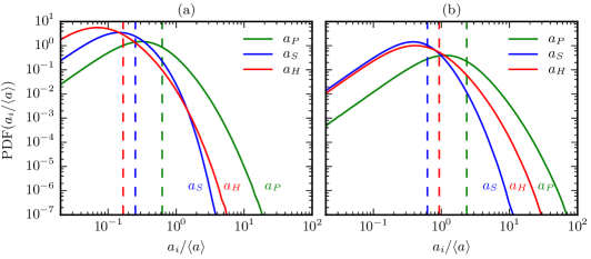
Figure 1: PDFs of the different accelerations $a_{i}$ due to the pressure gradient ($i=P$), the Stokes drag ($i=S$) and the history force ($i=H$). The particle parameters are (a) $\varrho=2$, $St=0.5$ ($r/\eta=0.95$) and (b) $\varrho=0$, $St=0.5$ ($r/\eta=2.1$) . The vertical lines show the positions of the averages: $\left\langle a_{P}\right\rangle/\left\langle a\right\rangle=0.62$, $\left\langle a_{S}\right\rangle/\left\langle a\right\rangle=0.25$, $\left\langle a_{H}\right\rangle/\left\langle a\right\rangle=0.17$ in (a) and $\left\langle a_{P}\right\rangle/\left\langle a\right\rangle=2.4$, $\left\langle a_{S}\right\rangle/\left\langle a\right\rangle=0.62$, $\left\langle a_{H}\right\rangle/\left\langle a\right\rangle=0.93$ in (b).

Figures 1a and 1b show the probability density functions (PDFs) of $a_{P}$, $a_{S}$ and $a_{H}$ for particles heavier ($\varrho=2$) and lighter ($\varrho=0$) than the fluid. In both cases $a_{P}$ is the dominant contribution, followed by $a_{S}$ and $a_{H}$. The Stokes drag and the history force are of similar magnitude showing that the history force is a viscous effect which can be as important as the drag. In these particular cases we find $\left\langle a_{H}\right\rangle/\left\langle a_{S}\right\rangle=66\%$ in figure 1a and $\left\langle a_{H}\right\rangle/\left\langle a_{S}\right\rangle=150\%$ in figure 1b. Additionally the PDF of the history force has longer tails than that of the Stokes drag (see figure 1a and also note that the $x$-axis is logarithmic), i.e. the history force has more extreme events.

Let us now consider the relative importance of the history force and compare it to the Stokes drag by means of the ratio $a_{H}/a_{S}$. Before proceeding to the numerical simulations, let us try to obtain an estimate of this ratio. To this end we apply the approximation

$$\left(\frac{\mathrm{d}}{\mathrm{d}t}\right)^{1/2}\left(\boldsymbol{v}-\boldsymbol{u}\right)\approx\frac{\alpha}{\sqrt{\tau_{\eta}}}\left(\boldsymbol{v}-\boldsymbol{u}\right),$$ (7)

which is motivated by the fact that the history force is a (fractional) time-derivative. The choice of $\tau_{\eta}$ as the characteristic time scale of $\boldsymbol{v}-\boldsymbol{u}$ seems natural as the particle “lives” on the small scales and should follow the flow to some degree (except for very large $St$). The constant $\alpha$ is expected to be on the order of unity. With this approximation and the definition of $a_{H}$ and $a_{S}$ we obtain an estimate for the relative magnitude of the history force (see also Daitche & Tél (2014)):

$$\frac{a_{H}}{a_{S}}\approx\alpha\sqrt{\frac{3\beta\tau_{p}}{\tau_{\eta}}}=\alpha\frac{r}{\eta}.$$ (8)

Thus we expect the importance of the history force to scale solely with the particle size and to be independent of its density.

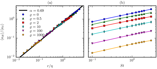
Figure 2: The ratio of the average magnitude of the history force and the Stokes drag as a function of (a) $r/\eta$ and (b) $St$.

Figure 2a shows $\left\langle a_{H}\right\rangle/\left\langle a_{S}\right\rangle$, measured in the turbulence simulations, as a function of $r/\eta$. We see a collapse of the data for different densities, which confirms our expectation that the particle size is the determining parameter for the relative magnitude of the history force. (When looking more closely we actually see a very weak dependence on the density, the collapse is not perfect.) A fit of our prediction (8) to the data yields $\alpha=0.69$ and we see that this simple estimate holds quite well.

Figure 2b shows $\left\langle a_{H}\right\rangle/\left\langle a_{S}\right\rangle$ as a function of the Stokes number. In this case there is no collapse for different densities and the relative magnitude of the history force decays with growing density. This tendency is true for a fixed Stokes number. Because $St$ depends on both the density and the particle size, increasing $\varrho$ and holding $St$ fixed means that we implicitly decrease the particle size. Thus the dependence on $\varrho$ in figure 2b is actually a disguised dependence on $r$. That there is no “real” dependence on $\varrho$ can be concluded from figure 2a.

We are now able to make an informed categorization of the importance of the history force based on its relative magnitude. For $r/\eta$ around $10^{-2}$ or less its contribution is very small (less than 1%) and should be negligible in most cases. For $r/\eta$ around $0.1$ the contribution is around 7%; while not negligible the history force is expected to play a minor role. For $r$ on the order of $\eta$ the contribution of the history force is on the order of the Stokes drag and is thus expected to be important for the particle motion.

4 Slip velocity

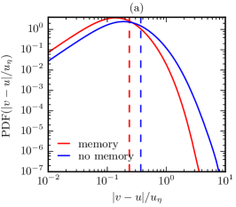
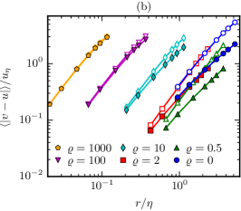
Figure 3: (a) PDFs of the slip velocity for particles with and without memory for $\varrho=2$ and $St=0.5$ ($r/\eta=0.95$). The vertical lines show the position of the averages: $\left\langle\left|\boldsymbol{v}-\boldsymbol{u}\right|/u_{\eta}\right\rangle_{\text{memory}}=0.24$ and $\left\langle\left|\boldsymbol{v}-\boldsymbol{u}\right|/u_{\eta}\right\rangle_{\text{no memory}}=0.37$. (b) The average slip velocity with (filled symbols) and without memory (unfilled symbols) as a function of the particle size and for different particle densities.

Now that we can estimate the magnitude of the history force, let us turn to its effects on the particle dynamics. A basic property of inertial particles is that they can deviate from the fluid flow (in contrast to tracers). It is thus natural to study the effect of the history force on this deviation, namely on the slip velocity $\boldsymbol{v}-\boldsymbol{u}$. Figure 3a shows the PDF of $\left|\boldsymbol{v}-\boldsymbol{u}\right|$ with and without the history force (denoted by “memory” and “no memory” respectively). Memory leads to a reduction of the slip velocity; in this case the mean slip velocity is reduced by 35% in comparison to the case without memory. Also, the tails of the PDF become shorter, i.e., strong detachments from the flow occur less frequently with memory. Figure 3b presents an overview of the full parameter space, showing the average slip velocity with and without memory. The natural parameter for the slip velocity is the Stokes number, however to make the role of the size clearer the data are shown as a function of $r/\eta$. We see that the effect of the history force (the difference between the case with and without memory) increases with $r$.

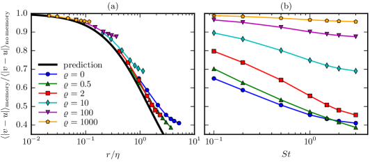
Figure 4: The ratio of the average slip velocity with and without memory as a function of (a) $r/\eta$ and (b) $St$.

To obtain a compact representation of this effect of memory let us use the ratio $\left|\boldsymbol{v}-\boldsymbol{u}\right|_{\mathrm{memory}}/\left|\boldsymbol{v}-\boldsymbol{u}\right|_{\mathrm{no\,memory}}$, i.e. the slip velocity with the history force divided by the one without. Before proceeding to the data from the simulations let us first try to obtain an analytical estimate. Using the equation of motion (2) and the approximation (7) we can estimate the slip velocity as

$$\boldsymbol{v}-\boldsymbol{u}\approx\left(\beta\frac{\mathrm{D}\boldsymbol{u}}{\mathrm{D}t}-\frac{\mathrm{d}\boldsymbol{v}}{\mathrm{d}t}\right)\left(\frac{1}{\tau_{p}}+\alpha\sqrt{\frac{3\beta}{\tau_{p}\tau_{\eta}}}\right)^{-1}=\left(\beta\frac{\mathrm{D}\boldsymbol{u}}{\mathrm{D}t}-\frac{\mathrm{d}\boldsymbol{v}}{\mathrm{d}t}\right)\frac{\tau_{p}}{1+\alpha\frac{r}{\eta}},$$ (9)

where the case without memory is contained for $\alpha=0$. If we assume that the first factor on the right-hand side of (9) is the same for both cases we obtain

$$\frac{\left|\boldsymbol{v}-\boldsymbol{u}\right|_{\mathrm{memory}}}{\left|\boldsymbol{v}-\boldsymbol{u}\right|_{\mathrm{no\,memory}}}\approx\frac{1}{1+\alpha\frac{r}{\eta}}.$$ (10)

Parameter $\alpha$ was introduced in section 3, where its value was determined from the numerical simulations: $\alpha=0.69$. Thus (10) provides a prediction for the slip velocity ratio. Figure 4a shows the ratio $\left\langle\left|\boldsymbol{v}-\boldsymbol{u}\right|\right\rangle_{\mathrm{memory}}/\left\langle\left|\boldsymbol{v}-\boldsymbol{u}\right|\right\rangle_{\mathrm{no\,memory}}$ obtained from the simulations along with this prediction. Although not perfect, this estimate – based on rather simple assumptions – fits reasonably well to the simulations (note that the black line in figure 4a is not a fit of (10) to the data; we used the previously obtained value of $\alpha$). An important observation is that the slip velocity ratio collapses for different densities when considered as a function of $r$. Although this collapse is not perfect (there seems to be a systematic deviation for $St>1$), it is still remarkable that the density plays only a minor role also for the effect of memory on the slip velocity. When the slip velocity ratio is considered as a function of $St$, there is no collapse at all, see figure 4b.

This result suggests again that the natural parameter for the effect of the history force is the particle size. Due to its simplicity, formula (10), as well as (8), can be very useful for estimates of this effect (when $\alpha$ is not known, one might assume $\alpha\approx 1$).

The findings of this section support the categorization of the memory effect for different particle sizes given at the end of the previous section. For $r/\eta\leq 10^{-2}$ the effect is negligible as the relative reduction of the slip velocity ( $1-\left\langle\left|\boldsymbol{v}-\boldsymbol{u}\right|\right\rangle_{\mathrm{memory}}/\left\langle\left|\boldsymbol{v}-\boldsymbol{u}\right|\right\rangle_{\mathrm{no\,memory}}$) is below 1%. For $r/\eta\approx 0.1$ the reduction is around 5%, i.e. not completely negligible but still small. For $r/\eta\approx 1$ it is around 35% and thus considerable.

5 Acceleration

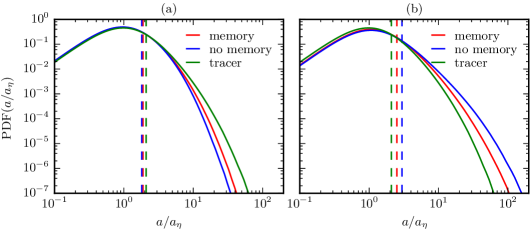
Figure 5: PDFs of the magnitude of the acceleration for particles with and without memory and tracers. The particle parameters are (a) $\varrho=2$, $St=0.5$ ($r/\eta=0.95$) and (b) $\varrho=0$, $St=0.5$ ($r/\eta=2.1$). The vertical lines show the positions of the averages: $\left\langle a/a_{\eta}\right\rangle_{\text{tracer}}=2.1$ and $\left\langle a/a_{\eta}\right\rangle_{\text{memory}}=1.9$, $\left\langle a/a_{\eta}\right\rangle_{\text{no memory}}=1.8$ in (a) and $\left\langle a/a_{\eta}\right\rangle_{\text{memory}}=2.5$, $\left\langle a/a_{\eta}\right\rangle_{\text{no memory}}=3.0$ in (b).

Let us now turn to the influence of the history force on the particle acceleration, a much studied quantity in turbulence research. Figures 5a and 5b show the PDFs of the modulus of the acceleration for particles with and without memory and tracers. For heavy particles (figure 5a) the history force increases the acceleration: the average increases slightly and the tails more notably (note the logarithmic $x$-axis). For light particles (figure 5b) the effect is opposite, the history force decreases the acceleration. The change of the mean acceleration is stronger in this case. We can describe these observations in a unified way: the acceleration PDF with memory comes closer to that of tracers (compare figures 5a and 5b).

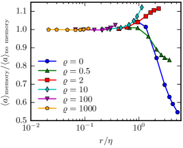
Figure 6: The ratio of the averaged acceleration magnitudes with and without memory.

To obtain an overview of the parameter dependence we again turn to ratios. Figure 6 shows the ratio of the (averaged) magnitudes of acceleration with and without memory. We see that the history force generally increases the acceleration of heavy particles and decreases the acceleration of light particles, as we found in two particular cases above. This effect is noticeable but not very large, except for $\varrho=0$ and large particle sizes. Note that there is no collapse of the ratios shown in figure 6 in contrast to the slip velocity ratio shown in figure 4a and the force ratio shown in figure 2a. Although the influence of memory generally increases with $r$ also for this observable, there is additionally a clear dependence on the density.

6 Preferential concentration

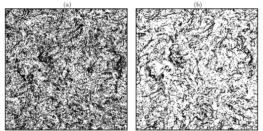
Figure 7: The distribution of light particles (a) with and (b) without memory. Both plots show the positions of $5\cdot 10^{4}$ particles contained in the slab $\left[0,L_{\mathrm{box}}\right]\times\left[0,L_{\mathrm{box}}\right]\times\left[0,L_{\mathrm{box}}/10\right]$ at $t=291\tau_{\eta}$ (this corresponds to 10 large-eddy-turnover times). The particles were homogeneously distributed at the beginning of the simulation and have the parameters $\varrho=0$ and $St=0.5$.

A much studied phenomenon concerning inertial particles is preferential concentration: the tendency of particles to gather in certain regions of the flow. Figure 7 shows the distribution of light particles with and without memory. In both cases we can see an inhomogeneous distribution of particles, i.e. preferential concentration. We also clearly see that the preferential concentration is weaker with the history force (figures 7a and 7b show the same number of particles).

To obtain an overview of the parameter dependence of this effect we need to quantify preferential concentration. There are several possible approaches; we use the correlation dimension $D_{2}$ as introduced by Grassberger & Procaccia (1983). Let $P(R)$ be the probability to find a given particle pair with a distance below $R$, i.e.

$$P(R)=\left\langle\Theta\left(R-\left|\boldsymbol{x}_{1}-\boldsymbol{x}_{2}\right|\right)\right\rangle,$$ (11)

where $\Theta$ is the Heaviside function and $\boldsymbol{x}_{1}$, $\boldsymbol{x}_{2}$ the positions of the two particles. Then the correlation dimension is defined through

$$P(R)\propto R^{D_{2}}\quad R\rightarrow 0.$$ (12)

In studies of preferential concentration the radial distribution function $g(R)$ is frequently used. It is closely related to $P(R)$ and $D_{2}$ ($d$ is the space dimension):

$$g(R)\propto\frac{\partial_{R}P(R)}{R^{d-1}}\propto R^{D_{2}-d},$$ (13)

see e.g. Bec et al. (2005). Thus $D_{2}$ can also be seen as a characterization of the radial distribution function.

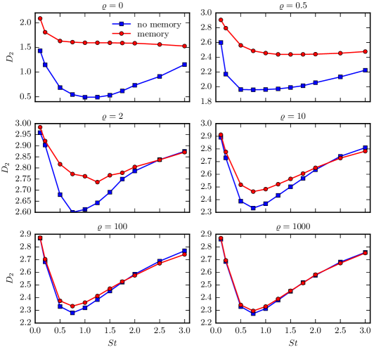
Figure 8: The correlation dimension $D_{2}$ of the particle distribution in space as a function of $St$ for different densities with and without memory.

To determine $D_{2}$ we measured $P(R)$ in our simulations and fitted a power law in the range $R/\eta\in\left[10^{-1},10\right]$. Figure 8 shows the correlation dimension as a function of the Stokes number for different densities. Without memory we see the typical unimodal shape of $D_{2}(St)$ found in previous studies, e.g. Calzavarini et al. (2008). The minimal value of $D_{2}$, corresponding to maximal preferential concentration, is obtained around $St\approx 1$. Concerning the influence of the history force we find: for $\varrho=1000$ there is hardly any effect; for $\varrho=100$ there is a small effect; for $\varrho=2$ and $\varrho=10$ the effect is quite noticeable; for light particles ($\varrho=0$ and $\varrho=0.5$) the effect is strong, e.g. for $\varrho=0$ the smallest value of $D_{2}$ increases by $1.1$ when memory is included – a very considerable change for a fractal dimension. It is interesting to note that the position of the smallest $D_{2}$ is shifted by the history force for $\varrho=2$; for $\varrho=0.5$ and $\varrho=0$ there does not seem to be a clear minimum with memory but rather an extended plateau. Also note that the influence of memory is strongest where $D_{2}$ attains its minimum. To sum up, if we fix the Stokes number and decrease $\varrho$, the effect of the history force on $D_{2}$ and thus on preferential concentration increases and becomes very strong for small densities.

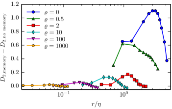
Figure 9: The change in the correlation dimension $D_{2}$ due to memory as a function of the particle size and density.

Note that for a fixed Stokes number we cannot discern the dependencies of this effect on $r$ and $\varrho.$ As $St$ depends on both parameters, varying $\varrho$ implicitly varies $r$; in particular, decreasing $\varrho$ increases $r$, see (3)-(5). Thus the dependence on $\varrho$ in figure 8 might be a disguised dependence on $r$ (as is the case in figure 2b for the relative magnitude of the history force and in figure 4b for the slip velocity ratio). Thus we have to consider this effect as a function of the particle size and density to discern the dependencies. Figure 9 shows the change of the correlation dimension $D_{2,\mathrm{memory}}-D_{2,\mathrm{no\ memory}}$ as a function of these two variables. We see a dependence on both $r$ and $\varrho$. This is in contrast to the behaviour of the relative magnitude of the history force (section 3) and the slip velocity ratio (section 4), where the determining parameter was solely $r$ and similar to the case of the acceleration (previous section). Note also that the dependence on $r$ and $\varrho$ is quite non-trivial, e.g. it is non-monotonic in both variables.

A good way to summarize these findings is as follows: For a fixed Stokes number the influence of the history force increases monotonically when the particle density decreases or (equivalently) when the particle size increases. However, one has to keep in mind that this dependency cannot be attributed to only one of the two parameters.

7 Collision rates

The collision rate of particles in turbulent flows is important for the understanding of, e.g., cloud microphysics or aggregation processes; it is also closely related to preferential concentration. One of the main findings in this area is that turbulence can enhance the collision rate enormously. We will study here the effect of the history force on the collision rate.

Let $N_{c}(t,\Delta\tau)$ be the number of particle collisions during a small time interval $\left[t,t+\Delta\tau\right]$, then the collision rate per unit volume is

$$R(t)=\frac{N_{c}(t,\Delta\tau)}{L_{\mathrm{box}}^{3}\Delta\tau}.$$ (14)

This quantity is independent of $t$ in stationary turbulence, but grows quadratically with the particle number density $n=N_{p}/L_{\mathrm{box}}^{3}$. A quantity where this dependence is factored out is the collision kernel

$$\Gamma=\frac{2R}{n^{2}},$$ (15)

which we will use in the following.

To obtain $N_{c}(t,\Delta\tau)$ we have simulated an ensemble of $N_{p}=5\cdot 10^{5}$ particles for every parameter value and saved snapshots of the particle positions every $\Delta\tau=0.2\tau_{\eta}$ time units. The collisions have been determined using the so-called ghost collision approximation, i.e. in our simulations the particles do not interact on contact but simply slip through each other. A collision is considered to occur when the distance between two particles becomes less then $2r$. To determine the occurrence of such events, the particle trajectories have been interpolated linearly in between the saved snapshots.

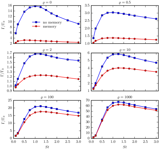
Figure 10: The collision kernel $\Gamma$ as a function of the Stokes number for different densities with and without memory. It is normalized by $\Gamma_{0}=\sqrt{8\pi/15}(2r)^{3}/\tau_{\eta}$ the collision kernel based on the dynamics of tracers, as derived by Saffman & Turner (1956).

Figure 10 shows the collision kernel as a function of the Stokes number for different densities. We see that the inclusion of the history force leads to a decrease in the collision rate. This effect is very strong for small densities and decreases for denser particles (when $St$ is fixed). The general picture is quite similar to that of the previous section where preferential concentration was studied and we see that memory can be important in determining the collision rate of inertial particles.

An interesting difference to the case of preferential concentration is that for large $\varrho$ the influence of memory on collision rates is stronger than on preferential concentration (compare figures 8 and 10). For example at $\varrho=1000$ and $St=1$ there is a very small change in $D_{2}$ due to memory but a more noticeable one in $\Gamma$ (8% relative change). The collision rate in turbulence is generally believed to be influenced by two effects: preferential concentration and caustics (also called sling effect), see e.g. Voßkuhle et al. (2014). Therefore this larger increase in the collision rate, as compared to preferential concentration, might be due to an influence of the history force on caustics; or more specifically, on the relative velocity of colliding particles.

As detailed in the last section, we are not able to discern the roles of $r$ and $\varrho$ when $St$ is fixed, as is the case in figure 10. This can be only done by looking at the change of $\Gamma$ as a function of $r$ and $\varrho$, as has been done for the correlation dimension in figure 9. In the analogous figure for $\Gamma_{\mathrm{memory}}/\Gamma_{\mathrm{no\,memory}}$ (not shown here) one observes a similar picture: the influence of memory depends on both $r$ and $\varrho$. The summary of the findings for collision rates is similar as well: for a fixed Stokes number the influence of memory increases monotonically when the particles density decreases or (equivalently) when the particle size increases.

8 Comparison with the work of Olivieri et al. (2014)

Recently Olivieri et al. (2014) published a study of the history force in turbulence. During the preparation of the present work discrepancies with this publication have been found. The type of flow used by Olivieri et al. (2014) is very similar to ours, therefore we present here a detailed quantitative comparison. We note that there is a difference in the methods of forcing the turbulence, which might be a cause of the discrepancies. Our forcing (which is described in appendix D) varies on a large time scale while the forcing by Olivieri et al. (2014) changes randomly at every time step (L. Brandt, private communication, 2014), i.e. the flow and the particles are forced on small time scales.

Olivieri et al. (2014) analyse the contributions of different forces to the whole acceleration of the particle. In our notation their quantities are

$$\boldsymbol{a}_{\textsc{pg}} =\frac{1}{\varrho}\frac{\mathrm{D}\boldsymbol{u}}{\mathrm{D}t}$$ (16)

$$\boldsymbol{a}_{\textsc{am}} =\frac{1}{2\varrho}\left(\frac{\mathrm{D}\boldsymbol{u}}{\mathrm{D}t}-\frac{\mathrm{d}\boldsymbol{v}}{\mathrm{d}t}\right)$$ (17)

$$\boldsymbol{a}_{\textsc{sd}} =\xi\frac{\boldsymbol{u}-\boldsymbol{v}}{\tau_{p}}$$ (18)

$$\boldsymbol{a}_{\textsc{ba}} =\xi\sqrt{\frac{3\beta}{\tau_{p}}}\left(\frac{\mathrm{d}}{\mathrm{d}t}\right)^{1/2}\left(\boldsymbol{u}-\boldsymbol{v}\right)$$ (19)

representing the pressure gradient, the added mass, the Stokes drag and the (Basset) history force. The factor $\xi=\tau_{p}/\tau_{p}^{\prime}=\left(2\varrho+1\right)/(2\varrho)$ accounts for the slightly different definition of the particle response time by Olivieri et al. (2014): $\tau_{p}^{\prime}=2\varrho r^{2}/(9\nu)$. We will use the corresponding Stokes number $St^{\prime}=\tau_{p}^{\prime}/\tau_{\eta}=St/\xi$ for the particle parameters in this section. Note that $\xi$ and $\beta$ are shorthand notations for certain combinations of $\varrho$ and that these three quantities are equivalent to each other.

To quantify the contributions of the different forces Olivieri et al. (2014) consider the component-wise ratios of the accelerations given above and the full particle acceleration $\boldsymbol{a}\equiv\mathrm{d}\boldsymbol{v}/\mathrm{d}t=\boldsymbol{a}_{\textsc{pg}}+\boldsymbol{a}_{\textsc{am}}+\boldsymbol{a}_{\textsc{sd}}+\boldsymbol{a}_{\textsc{ba}}$:

$$\frac{a_{\textsc{pg},x}}{a_{x}},\,\frac{a_{\textsc{sd},x}}{a_{x}},\,\frac{a_{\textsc{ba},x}}{a_{x}}.$$ (20)

Because of the statistical isotropy of the underlying turbulent flow, it suffices to consider only one component (we choose the $x$-component). We omit here the contribution of the added mass effect as it is fully determined by pressure gradient contribution: $a_{\textsc{am},x}/a_{x}=\frac{1}{2}\left(a_{\textsc{pg},x}/a_{x}+1/\varrho\right)$.

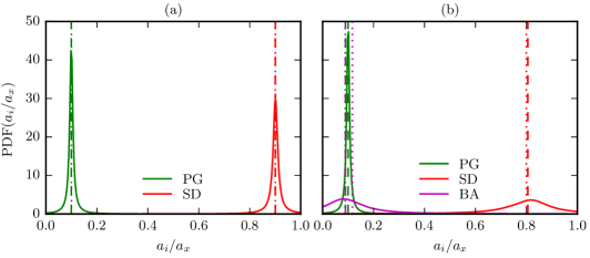
Figure 11: PDFs of the ratios $a_{i,x}/a_{x}$, $i\in\left\{\text{PG, SD, BA}\right\}$ for $\varrho=10$ and $St^{\prime}=0.1$ without (a) and with (b) memory. The vertical dashed lines show the positions of the averages of the PDFs. The average values predicted by the approximate formulas (25)-(27) are shown with vertical dotted lines.

Figure 11 shows the PDFs of the three ratios (20) for $\varrho=10$, $St^{\prime}=0.1$ in our simulations with and without memory. (Note that the choice of colours in the figures of this section is different from rest of the paper; it is the same as in (Olivieri et al. (2014)), to facilitate the comparison). Let us consider the case without memory first. It is shown in figure 11a and corresponds to figure $3a$ in (Olivieri et al. (2014)). When comparing those figures one sees a considerable difference. First, the mean values (represented by dashed lines) are different, e.g. in our simulations we find that the Stokes drag on average contributes to 90% of the particle acceleration while Olivieri et al. (2014) find 75%. Second, the PDFs obtained from our simulations are much sharper and well separated while in (Olivieri et al. (2014)) they are rather broad and overlap considerably. The case with memory is similar, compare our figure 11b and figure $3c$ in (Olivieri et al. (2014)). The mean value of $a_{\textsc{ba},x}/a_{x}$ (representing the contribution of the history force) found by Olivieri et al. (2014) is similar to the Stokes drag’s contribution while we find it to be much smaller. Note that the differences appear also for the case without memory and thus cannot stem solely from the treatment of the history force.

Let us get an independent estimate of the ratios (20). To this end we use the approximation (7) and the weakly inertial estimate for the slip velocity

$$\boldsymbol{u}-\boldsymbol{v}\approx\tau_{p}\left(1-\beta\right)\frac{\mathrm{D}\boldsymbol{u}}{\mathrm{D}t}$$ (21)

(which can be obtained by expanding (2) in powers of $\tau_{p}$ and keeping the linear terms, see e.g. Druzhinin & Ostrovsky (1994)) and obtain estimates for (18), (19) and the total acceleration

$$\boldsymbol{a}_{\textsc{sd}} \approx\xi\left(1-\beta\right)\frac{\mathrm{D}\boldsymbol{u}}{\mathrm{D}t}$$ (22)

$$\boldsymbol{a}_{\textsc{ba}} \approx\xi\alpha\frac{r}{\eta}\left(1-\beta\right)\frac{\mathrm{D}\boldsymbol{u}}{\mathrm{D}t}$$ (23)

$$\boldsymbol{a} \approx\left(1+\alpha\frac{r}{\eta}\left(1-\beta\right)\right)\frac{\mathrm{D}\boldsymbol{u}}{\mathrm{D}t}.$$ (24)

The case without memory is contained for $\alpha=0$. For the ratios (20) we get estimates which depend on the particle parameters and $\alpha$ only:

$$\frac{a_{\textsc{pg},x}}{a_{x}} \approx\frac{2}{3}\frac{\xi\beta}{1+\frac{r}{\eta}\alpha\left(1-\beta\right)}$$ (25)

$$\frac{a_{\textsc{sd},x}}{a_{x}} \approx\frac{\xi\left(1-\beta\right)}{1+\alpha\frac{r}{\eta}\left(1-\beta\right)}$$ (26)

$$\frac{a_{\textsc{ba},x}}{a_{x}} \approx\frac{\xi\alpha\frac{r}{\eta}\left(1-\beta\right)}{1+\alpha\frac{r}{\eta}\left(1-\beta\right)}$$ (27)

These estimates are shown in figure 11 as dotted lines. For the case without memory they coincide perfectly with the mean values obtained from the simulations (the dashed and dotted lines overlap). With memory the agreement between the estimate and the measured values is not perfect but still good. The main source of error here is probably the value of the coefficient $\alpha$. We thus see that the above estimates fit quite well to our simulations but not to the ones by Olivieri et al. (2014).

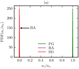
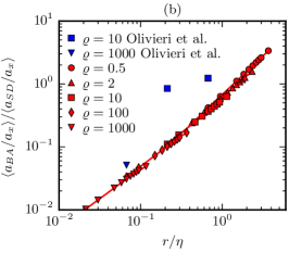
Figure 12: (a) PDFs of the ratios $a_{i,x}/a_{x}$ $i\in\left\{\text{PG, SD, BA}\right\}$ for $\varrho=1$ and $St^{\prime}=0.01$ with memory. (b) The ratio (28) as a function of the particle size from our simulations and those by Olivieri et al. (2014).

Let us come to the case of neutrally buoyant particles. Figure 12a shows the PDFs of the ratios (20) for $\varrho=1$ and $St^{\prime}=0.01$ with memory (without memory the picture is the same). The PDFs are sharp peaks around the values $0$ and $1$. We find that the contribution by the Stokes drag and the history force are negligible and basically the full contribution to the acceleration is from the pressure gradient $\boldsymbol{a}_{\textsc{pg}}$. This is expected for neutrally buoyant particles with very small Stokes numbers ($St^{\prime}=0.01$ here) as they should behave like tracers: with $\boldsymbol{v}=\boldsymbol{u}$ we get $\boldsymbol{a}_{\textsc{sd}}=\boldsymbol{a}_{\textsc{ba}}=0$, $\boldsymbol{a}=\boldsymbol{a}_{\textsc{pg}}=\mathrm{D}\boldsymbol{u}/\mathrm{D}t$ and thus $a_{\textsc{sd},x}/a_{x}=a_{\textsc{ba},x}/a_{x}=0$, $a_{\textsc{pg},x}/a_{x}=1$. This picture is very different in (Olivieri et al. (2014)), see their figure 4. The average contribution of the Stokes drag is far from zero and even larger than the contribution of the pressure gradient. Another strong difference is that the PDFs are rather broad in contrast to the sharp peaks found here.

To obtain an overview of the deviations (for $\varrho\neq 1$) let us consider the ratio

$$\frac{\left\langle a_{\textsc{ba},x}/a_{x}\right\rangle}{\left\langle a_{\textsc{sd},x}/a_{x}\right\rangle}$$ (28)

with the aim to describe the importance of the history force relative to the Stokes drag, akin to $\left\langle a_{H}\right\rangle/\left\langle a_{S}\right\rangle$ studied in section 3. Figure 12b shows the ratio (28) obtained from our simulations (the dependence on $r/\eta$ is similar to that in figure 2a) and compares these with three data points obtained from (Olivieri et al. (2014)). We see that the difference is considerable, the largest deviation is by almost one order of magnitude (for $\varrho=10$, $St^{\prime}=0.1$ and thus $r/\eta=0.21$).

To quantify preferential concentration Olivieri et al. (2014) use the radial distribution function $g(R)$ and find that memory reduces $g(R)$ and thus preferential concentration. Generally this is what we also find, but the amount of reduction is much smaller in our case. For example, at $St^{\prime}=1$ we find the relative reduction

$$1-\frac{g(R=r/\eta)_{\mathrm{memory}}}{g(R=r/\eta)_{\mathrm{no\,memory}}}$$ (29)

to be 25% for $\varrho=10$ and 3.5% for $\varrho=1000$ while Olivieri et al. (2014) find 52% and 23%, respectively.

To conclude, we see that there are strong differences between our results and those by Olivieri et al. (2014). A comparison with analytical estimates of the forces favours our results. From our perspective the simulations by Olivieri et al. (2014) seem to overestimate the importance of the history force. We note however that the conclusions by Olivieri et al. (2014) are similar to ours on a more general, qualitative level.

9 Summary and discussion

In the present paper we we have studied the importance of the the history force – a memory effect – for the motion of inertial particles in a turbulent flow. We have found that it can be quite important (depending on the particle parameters). Its effect is to reduce (i) the slip velocity, (ii) the difference in acceleration between inertial particles and tracers, (iii) the preferential concentration and (iv) the collision rate. We can concisely summarize these finds as follows: the history force causes inertial particles to stay closer to the flow and to behave more like tracers. This is in accordance with previous findings in a smooth flow with chaotic advection (Daitche & Tél (2011, 2014)).

How large the effects of memory are depends on the particle parameters. We have found simple approximative relations for the magnitude of the history force relative to the Stokes drag

$$\frac{a_{\mathrm{history\,force}}}{a_{\mathrm{Stokes\,drag}}}\approx\alpha\frac{r}{\eta}$$ (30)

and for the reduction of the slip velocity by memory

$$\frac{\left|\boldsymbol{v}-\boldsymbol{u}\right|_{\mathrm{memory}}}{\left|\boldsymbol{v}-\boldsymbol{u}\right|_{\mathrm{no\,memory}}}\approx\frac{1}{1+\alpha\frac{r}{\eta}}.$$ (31)

The constant $\alpha$ is expected to be on the order of unity and from numerical simulations we have determined $\alpha=0.69$. These relations make it possible to quickly obtain an estimate of the importance of the history force (when $\alpha$ is not known, setting $\alpha=1$ should still yield a reasonable estimate). The fact that these relations fit well to numerical simulations shows that for the magnitude of the history force and for the reduction of the slip velocity the determining parameter is the particle size and that the density is of minor importance.

This, however, is not true for all effects of memory. We have found the influence of the history force on particle acceleration, preferential concentration and collision rates to depend on both the particle size and density. In these cases we were not able to find simple estimates as above. A general summary of the findings on preferential concentration and collision rates is that for a fixed Stokes number a decreasing density or equivalently an increasing particle size lead to stronger effects of the history force. These effects can become quite strong for small densities/large sizes.

An important field of study for inertial particles is the motion of water droplets in air (e.g. in a cloud), where the density ratio $\varrho\approx 1000$ is very large. In this case we have found the effect of memory to be rather small. This is also true for the relative magnitude of the the history force and the reduction of the slip velocity, which do not depend on the particle’s density (at least approximately). At first this might seem contradictory but becomes clear when we note the following: we considered a fixed range of Stokes numbers ($St\in\left[0.1,3\right]$), the corresponding particle sizes for $\varrho=1000$ are quite small ($r/\eta\in\left[0.02,0.12\right]$) and hence also the effect of memory. It might, however, become more significant for larger $r/\eta$. Even within the investigated range, an interesting finding is that the change of the collision rate caused by the history force at $\varrho=1000$ and $St=1$ is 8%. Although this is still small, it is significantly larger than the effect on all other studied quantities for $\varrho=1000$. It remains to be seen whether this has any practical implications.

Valuable discussions with T. Tél, M. Wilczek, L. Brandt and J. Bec are acknowledged, as well as the support by the Studienstiftung des deutschen Volkes. The Eulerian part of the simulation code has been written by M. Wilczek.

Appendix A Faxén corrections in comparison to the history force

The aim of the present section is to compare the magnitudes of the Faxén corrections and the history force. We will see that the former is much smaller than the latter for most particle parameters considered in this paper.

With the Faxén corrections the evolution equation (2) becomes

$$\frac{\mathrm{d}\boldsymbol{v}}{\mathrm{d}t}=\beta\frac{\mathrm{D}}{\mathrm{D}t}\left(\boldsymbol{u}+\frac{r^{2}}{10}\Delta\boldsymbol{u}\right)-\frac{1}{\tau_{p}}\left(\boldsymbol{v}-\boldsymbol{u}-\frac{r^{2}}{6}\Delta\boldsymbol{u}\right)-\sqrt{\frac{3\beta}{\tau_{p}}}\left(\frac{\mathrm{d}}{\mathrm{d}t}\right)^{1/2}\left(\boldsymbol{v}-\boldsymbol{u}-\frac{r^{2}}{6}\Delta\boldsymbol{u}\right),$$ (32)

see Gatignol (1983); Maxey & Riley (1983). The full Faxén corrections are actually defined in terms of surface and volume integrals of $\boldsymbol{u}$ and $\mathrm{D}\boldsymbol{u}/\mathrm{D}t$. The $\Delta\boldsymbol{u}$ terms in (32), which are the commonly used forms of Faxén corrections, are the first non-vanishing terms of a Taylor expansion of these integrals. We restrict ourself here to these approximations (the full Faxén corrections have been considered by Calzavarini et al. (2012) in the case of neutrally buoyant particles through a special numerical scheme). The second limitation of our comparison is that we do not solve (32) but equation (2) without Faxén corrections and only afterwards evaluate $\Delta\boldsymbol{u}$ along the particle trajectories. Our aim is to obtain a rough comparison of the typical magnitudes of the Faxén corrections and the history force; we expect that our approach, in spite of these limitations, is sufficient for this purpose.

In section 3 we have compared the history force to the drag and found a simple approximate rule for their ratio (8). We proceed in the same way for the Faxén corrections, by considering the ratio to the Stokes drag. The last two terms in (32) yield the ratio $\frac{r^{2}}{6}\left|\Delta\boldsymbol{u}\right|/\left|\boldsymbol{v}-\boldsymbol{u}\right|$. By approximating the slip velocity with

$$\boldsymbol{v}-\boldsymbol{u}\approx\tau_{p}\left(\beta-1\right)\frac{1}{1+\alpha\frac{r}{\eta}}\frac{\mathrm{D}\boldsymbol{u}}{\mathrm{D}t},$$ (33)

which follows from (9) with $\frac{\mathrm{d}\boldsymbol{v}}{\mathrm{d}t}\approx\frac{\mathrm{D}\boldsymbol{u}}{\mathrm{D}t}$, and using (4) we obtain

$$\frac{r^{2}}{6}\frac{\left|\Delta\boldsymbol{u}\right|}{\left|\boldsymbol{v}-\boldsymbol{u}\right|}\approx\frac{1}{2}\frac{\beta}{\left|\beta-1\right|}\left(1+\alpha\frac{r}{\eta}\right)\frac{\left|\nu\Delta\boldsymbol{u}\right|}{\left|\mathrm{D}\boldsymbol{u}/\mathrm{D}t\right|}.$$ (34)

Approximation (33) is similar to (21), but is of the slightly higher order 3/2 in $\tau_{p}$ (as $1/\left(1+\alpha r/\eta\right)\approx 1-\alpha r/\eta$ and $r\propto\sqrt{\tau_{p}}$). By averaging over tracers in our simulation we find

$$\frac{\left\langle\left|\nu\Delta\boldsymbol{u}\right|\right\rangle}{\left\langle\left|\mathrm{D}\boldsymbol{u}/\mathrm{D}t\right|\right\rangle}=0.14.$$ (35)

Because an average over tracers is equivalent to an Eulerian average, this ratio can be considered a property of the underlying flow, independent of the particle picture. Also, this results implies that the main contribution to $\mathrm{D}\boldsymbol{u}/\mathrm{D}t=-\nabla p+\nu\Delta\boldsymbol{u}$ is from $\nabla p$ and thus justifies the commonly used name “pressure gradient” for $\mathrm{D}\boldsymbol{u}/\mathrm{D}t$. Figure 13 shows the ratio $\frac{r^{2}}{6}\left\langle\left|\Delta\boldsymbol{u}\right|\right\rangle/\left\langle\left|\boldsymbol{v}-\boldsymbol{u}\right|\right\rangle$ obtained from simulations together with the approximation (34) for the numerical value (35). It fits quite well for $\varrho<10$. For $\varrho\geq 10$ there is a notable mismatch, nevertheless (34) provides a reasonable order of magnitude estimate.

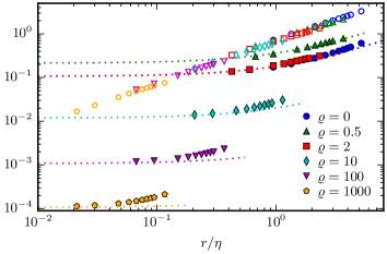
Figure 13: A comparison of the magnitudes of the Faxén corrections and the history force. Shown are the ratio $\frac{r^{2}}{6}\left\langle\left|\Delta\boldsymbol{u}\right|\right\rangle/\left\langle\left|\boldsymbol{v}-\boldsymbol{u}\right|\right\rangle$ (filled symbols), its approximation (34) (dotted lines) and the ratio $\left\langle a_{H}\right\rangle/\left\langle a_{S}\right\rangle$ (unfilled symbols).

Figure 13 also shows the ratio of the history force and the Stokes drag $\left\langle a_{H}\right\rangle/\left\langle a_{S}\right\rangle$, which was studied in section 3. We see that for all studied parameter values the magnitude of the Faxén corrections is smaller than the magnitude of the history force; in most cases it is much smaller. From all the considered densities the relative size of the Faxén corrections are largest at $\varrho=0.5$. This is expected because this value is closest to $\varrho=1$, in which case $\boldsymbol{v}\approx\boldsymbol{u}$ and thus the ratio $\frac{r^{2}}{6}\left|\Delta\boldsymbol{u}\right|/\left|\boldsymbol{v}-\boldsymbol{u}\right|$ becomes very large.

For for $\varrho=1$ we can expect $a_{H}\approx 0$ (see also appendix B) and because the Faxén corrections remain finite, they are expected to be much more important than the history force for neutrally buoyant particles (indeed even more important than the Stokes drag).

If we use the approximation (34) and extrapolate to smaller particles sizes, we see that the Faxén corrections become larger than the history force when $r$ is small enough. Indeed the ratio $\frac{r^{2}}{6}\left|\Delta\boldsymbol{u}\right|/\left|\boldsymbol{v}-\boldsymbol{u}\right|$ tends to a constant for $r\rightarrow 0$ while $a_{H}/a_{S}$ goes to zero, see figure 13. Thus for small $r$ (how small, depends on $\varrho$) the Faxén corrections become more important than the history force. However this is not the case for all of our studied parameter values. Also, when $\varrho$ is not close to $1$ both terms are quite small when the Faxén terms become more important; then both might be neglected.

Let us now come to the Faxén correction from the first term in (32). Using (33) we find the approximation

$$\frac{\beta\frac{\mathrm{D}}{\mathrm{D}t}\frac{r^{2}}{10}\Delta\boldsymbol{u}}{\frac{1}{\tau_{p}}\left|\boldsymbol{v}-\boldsymbol{u}\right|}\approx\frac{1}{10}\frac{\beta}{\left|\beta-1\right|}\left(\frac{r}{\eta}\right)^{2}\left(1+\alpha\frac{r}{\eta}\right)\frac{\left|\tau_{\eta}\frac{\mathrm{D}}{\mathrm{D}t}\nu\Delta\boldsymbol{u}\right|}{\left|\mathrm{D}\boldsymbol{u}/\mathrm{D}t\right|}$$ (36)

and for the unknown ratio

$$\frac{\left\langle\left|\tau_{\eta}\frac{\mathrm{D}}{\mathrm{D}t}\nu\Delta\boldsymbol{u}\right|\right\rangle}{\left\langle\left|\mathrm{D}\boldsymbol{u}/\mathrm{D}t\right|\right\rangle}=0.11$$ (37)

from simulations. Using this value and $\alpha=0.69$ (obtained in section 3) we can estimate that the Faxén correction from the first term in (32) is smaller than that form the second or third term when $r/\eta\leq 2.5$. Furthermore we find that the ratio (36) is smaller than $\left\langle a_{H}\right\rangle/\left\langle a_{S}\right\rangle$ for all the considered parameter values (i.e. those shown in figure 13).

We thus conclude that the magnitude of the Faxén corrections is smaller than the magnitude of the history force for all the investigated particle parameters; in most cases it is much smaller.

Appendix B Note on neutrally buoyant particles

Up to now we did not consider the case of neutrally buoyant particles. This case is special because trajectories of tracers, i.e. $\boldsymbol{v}=\boldsymbol{u}$, are valid solutions of (2) for $\varrho=1$. Indeed we have found in our simulations (for Stokes numbers $0.01$, $0.1$ and $1$) that neutrally buoyant particles behave very similar to tracers: the mean slip velocity is practically zero, the acceleration PDF is the same as for tracers, there is no preferential concentration and collision rates equal that of tracers (with an artificially assigned, corresponding radius). The inclusion of the history force does not change any of these findings and thus seems not to be important for neutrally buoyant particles.

We note that for larger particle sizes (not considered here) neutrally buoyant particles can behave differently from tracers; Calzavarini et al. (2012) have studied the effect of memory in this case (along with the influence of Faxén corrections and non-linear drag).

Concerning the forces acting on a particle, we find $\left\langle a_{S}\right\rangle\approx 0$ and $\left\langle a_{H}\right\rangle\approx 0$ for all studied Stokes numbers (see also figure 12a). Thus, the overwhelming contribution to the particle acceleration comes from the pressure gradient $a_{P}$. This does not mean that the Stokes drag is unimportant, because neglecting it (and the history force) in (2) would allow for solutions of the type $\boldsymbol{v}=\boldsymbol{u}+\boldsymbol{c}$ with an arbitrary constant $\boldsymbol{c}$, which is undesirable. One needs the Stokes drag as a restoring effect which keeps the particle close to a tracer trajectory (even though it has to act rarely). The history force can be also considered as a restoring effect (indeed it is sometimes called the unsteady drag). The fact that we do not find any influence of memory suggests that the Stokes drag is already sufficient to keep the particles very close to the tracer trajectories.

Note that we neglected the Faxén corrections in our simulations. This might be a serious limitation for neutrally buoyant particles as the findings of appendix A suggest. Thus the results of this section should to be treated with some caution.

A fundamental question concerning neutrally buoyant particles is whether the tracer solutions are stable, see e.g. Babiano et al. (2000); Sapsis & Haller (2008). The history force might play a very non-trivial role here. For example it was shown by Daitche & Tél (2011) that the history force can destroy attractors and that the convergence towards attractors becomes very slow ($\sim t^{-1/2}$) with memory. Thus a thorough study of the influence of memory on neutrally buoyant particles would have to include a stability analysis of tracer trajectories; this, however, is beyond the scope of this paper.

Appendix C A time-stepping scheme for particles with memory

Let us start by rewriting the evolution equation (2) for the slip velocity $\boldsymbol{w}=\boldsymbol{v}-\boldsymbol{u}$:

$$\frac{\mathrm{d}\boldsymbol{w}}{\mathrm{d}t} =\left(\beta-1\right)\frac{\mathrm{d}\boldsymbol{u}}{\mathrm{d}t}-\beta\boldsymbol{w}\cdot\nabla\boldsymbol{u}-\frac{1}{\tau_{p}}\boldsymbol{w}-\sqrt{\frac{3\beta}{\pi\tau_{p}}}\frac{\mathrm{d}}{\mathrm{d}t}\int_{0}^{t}\frac{\boldsymbol{w}}{\sqrt{t-\tau}}\,\mathrm{d}\tau$$ (38)

$$\frac{\mathrm{d}\boldsymbol{x}}{\mathrm{d}t} =\boldsymbol{w}+\boldsymbol{u},$$ (39)

where $\mathrm{d}\boldsymbol{u}/\mathrm{d}t=\partial_{t}\boldsymbol{u}+\boldsymbol{v}\cdot\nabla\boldsymbol{u}$. We wish to obtain a numerical solution at the time points $t_{n}=nh$, where $h$ is the time step. Integrating (38) from $t_{n}$ to $t_{n+1}$ we get

$$\boldsymbol{w}_{n+1}=\boldsymbol{w}_{n}+\left(\beta-1\right)\left(\boldsymbol{u}_{n+1}-\boldsymbol{u}_{n}\right)-\beta\int_{t_{n}}^{t_{n+1}}\boldsymbol{w}\cdot\nabla\boldsymbol{u}\,\mathrm{d}\tau-\frac{1}{\tau_{p}}\int_{t_{n}}^{t_{n+1}}\boldsymbol{w}\,\mathrm{d}\tau\\ +\xi\int_{0}^{t_{n+1}}\frac{\boldsymbol{w}}{\sqrt{t_{n+1}-\tau}}\,\mathrm{d}\tau-\xi\int_{0}^{t_{n}}\frac{\boldsymbol{w}}{\sqrt{t_{n}-\tau}}\,\mathrm{d}\tau$$ (40)

where $\xi=-\sqrt{3\beta/(\pi\tau_{p})}$. To obtain a numerical stepping scheme we have to approximate the integrals. We begin with the first two:

$$\int_{t_{n}}^{t_{n+1}}f(\tau)\mathrm{d}\tau\approx h\sum_{i=0}^{m}\lambda_{i}^{(m)}f(\tau_{n+1-i})$$ (41)

The coefficients $\lambda_{i}^{(m)}$ are well known. For an explicit scheme, i.e. $\lambda_{0}=0$, they are the coefficients $\boldsymbol{\lambda}^{B,m}$ of the Adams-Bashforth schemes:

$$\boldsymbol{\lambda}^{B,2} = \left(0,1\right)$$ (42)

$$\boldsymbol{\lambda}^{B,3} = \left(0,\frac{3}{2},-\frac{1}{2}\right)$$ (43)

$$\boldsymbol{\lambda}^{B,4} = \left(0,\frac{23}{12},-\frac{4}{3},\frac{5}{12}\right)$$ (44)

For an implicit scheme they are the coefficients $\boldsymbol{\lambda}^{M,m}$ of the Adams-Moulton schemes:

$$\boldsymbol{\lambda}^{M,2} = \left(\frac{1}{2},\frac{1}{2}\right)$$ (45)

$$\boldsymbol{\lambda}^{M,3} = \left(\frac{5}{12},\frac{8}{12},-\frac{1}{12}\right)$$ (46)

The errors of these approximations are $O(h^{m})$ for $\boldsymbol{\lambda}^{B,m}$ and $O(h^{m+1})$ for $\boldsymbol{\lambda}^{M,m}$. The history integrals in (40) are approximated with

$$\int_{0}^{t_{n}}\frac{\boldsymbol{w}}{\sqrt{t-\tau}}\mathrm{d}\tau\approx\sqrt{h}\sum_{i=0}^{n}\mu_{i}\boldsymbol{w}_{n-i}$$ (47)

where $\boldsymbol{w}_{n}=\boldsymbol{w}(t_{n})$ and the coefficients $\mu_{i}$ are given by Daitche (2013). We thus obtain the following scheme for the slip velocity:

$$\boldsymbol{w}_{n+1}=\boldsymbol{w}_{n}+\left(\beta-1\right)\left(\boldsymbol{u}_{n+1}-\boldsymbol{u}_{n}\right)-\beta h\sum_{i=0}^{m}\lambda_{i}^{B,m}\left[\boldsymbol{w}\cdot\nabla\boldsymbol{u}\right]_{n+1-i}-\frac{h}{\tau_{p}}\sum_{i=0}^{m}\lambda_{i}^{M,m}\boldsymbol{w}_{n+1-i}\\ +\xi\sqrt{h}\left(\sum_{i=0}^{n+1}\mu_{i}\boldsymbol{w}_{n+1-i}-\sum_{i=0}^{n}\mu_{i}\boldsymbol{w}_{n-i}\right)$$ (48)

Note that the right-hand side contains $\boldsymbol{w}_{n+1}$, but only linearly. Bringing it to the left-hand side yields an explicit scheme:

$$\left(1+\frac{h}{\tau_{p}}\lambda_{0}^{M}-\xi\sqrt{h}\mu_{0}\right)\boldsymbol{w}_{n+1} = \boldsymbol{w}_{n}+\left(\beta-1\right)\left(\boldsymbol{u}_{n+1}-\boldsymbol{u}_{n}\right)$$ (49)

$$-\beta h\sum_{i=0}^{m}\lambda_{i}^{B,m}\left[\boldsymbol{w}\cdot\nabla\boldsymbol{u}\right]_{n+1-i}-\frac{h}{\tau_{p}}\sum_{i=1}^{m}\lambda_{i}^{M,m}\boldsymbol{w}_{n+1-i}$$

$$+\xi\sqrt{h}\left(\sum_{i=1}^{n+1}\mu_{i}\boldsymbol{w}_{n+1-i}-\sum_{i=0}^{n}\mu_{i}\boldsymbol{w}_{n-i}\right)$$

$$\boldsymbol{x}_{n+1} = \boldsymbol{x}_{n}+h\sum_{i=0}^{m}\lambda_{i}^{B,m}\left(\boldsymbol{w}_{n+1-i}+\boldsymbol{u}_{n+1-i}\right)$$ (50)

Using $\lambda_{i}^{B,4}$, $\lambda_{i}^{M,3}$ and the third-order coefficients $\mu_{i}$ from (Daitche (2013)) the above scheme has a one-step error of $O(h^{4})$, i.e. it is a third-order scheme.

As this scheme relies on previous values of $\boldsymbol{x}$ and $\boldsymbol{w}$, one needs to start the integration with lower order schemes: the first step with $\lambda_{i}^{B,2}$, $\lambda_{i}^{M,1}$ and the first-order $\mu_{i}$; the second step with $\lambda_{i}^{B,3}$, $\lambda_{i}^{M,2}$ and the second-order $\mu_{i}$.

To further improve the accuracy of the scheme, corrector steps have been applied. A corrector step is performed by predicting $\boldsymbol{x}_{n+1}$, $\boldsymbol{w}_{n+1}$ with the explicit scheme (49)-(50), replacing the $\lambda_{i}^{B}$ in this scheme with $\lambda_{i}^{M}$ (thus making it implicit), inserting the predicted $\boldsymbol{x}_{n+1}$, $\boldsymbol{w}_{n+1}$ in the right-hand side and calculating a corrected estimate for $\boldsymbol{x}_{n+1}$, $\boldsymbol{w}_{n+1}$. (The corrector steps are not essential for the numerical scheme.)

That the one-step error of this scheme scales indeed with $h^{4}$, has been verified in a case where an analytical solution of (2) is available: a particle moving in a two dimensional vortex (Candelier et al. (2004)), see also (Daitche (2013)).

Appendix D Forcing the turbulence

We solve the vorticity equation in a triply periodic box of length $L_{\mathrm{box}}=2\pi$. In Fourier space the equation becomes

$$\partial_{t}\boldsymbol{\omega}_{\boldsymbol{k}}=i\boldsymbol{k}\times\mathcal{F}[\boldsymbol{u}\times\boldsymbol{\omega}]_{\boldsymbol{k}}-\nu\boldsymbol{k}^{2}\boldsymbol{\omega}_{\boldsymbol{k}}+\boldsymbol{F}_{\boldsymbol{k}}.$$ (51)

Here $\boldsymbol{\omega}=\nabla\times\boldsymbol{u}$ is the vorticity, $\boldsymbol{k}\in\mathbb{Z}^{3}$ the wave vector, $\mathcal{F}$ the Fourier transform and $\boldsymbol{F}$ the forcing. The latter is implicitly defined as described in the following. We force by inserting the energy lost during one time step back into large scale modes $\boldsymbol{\omega}_{\boldsymbol{k}}$ with $\boldsymbol{k}$ in the forcing band

$$B=\left\{\boldsymbol{k}\left|3\leq\boldsymbol{k}^{2}\leq 9\right.\right\}.$$ (52)

Let $\boldsymbol{\omega}_{\boldsymbol{k}}^{n}$ be the current vorticity and $\tilde{\boldsymbol{\omega}}_{\boldsymbol{k}}^{n+1}$ the vorticity after one time step without forcing (more precisely, when using a scheme consisting of multiple stages, like a Runge-Kutta method, $\tilde{\boldsymbol{\omega}}_{\boldsymbol{k}}^{n+1}$ is the vorticity after one stage). The forcing is applied by rescaling the modes in the forcing band:

$$\boldsymbol{\omega}_{\boldsymbol{k}}^{n+1}=\begin{cases}f\tilde{\boldsymbol{\omega}}_{\boldsymbol{k}}^{n+1}&\boldsymbol{k}\in B\\ \tilde{\boldsymbol{\omega}}_{\boldsymbol{k}}^{n+1}&\boldsymbol{k}\notin B\end{cases}$$ (53)

The factor $f$ is chosen such that the energy of the flow

$$E\left[\boldsymbol{\omega}_{\boldsymbol{k}}\right]=\frac{1}{2}\sum_{\boldsymbol{k}}\frac{\left|\boldsymbol{\omega}_{\boldsymbol{k}}\right|^{2}}{\boldsymbol{k}^{2}}$$ (54)

remains constant, i.e.

$$E\left[\boldsymbol{\omega}_{\boldsymbol{k}}^{n+1}\right]=E\left[\boldsymbol{\omega}_{\boldsymbol{k}}^{n}\right].$$ (55)

The modes$\left\{\left.\boldsymbol{\omega}_{\boldsymbol{k}}\right|\boldsymbol{k}\notin B\right\}$ evolve freely and the energy is kept constant by inserting energy into the modes $\left\{\left.\boldsymbol{\omega}_{\boldsymbol{k}}\right|\boldsymbol{k}\in B\right\}$. Note also that only the modulus of the modes is modified, their direction can evolve freely, which improves the statistical isotropy of the flow.

References

- van Aartrijk & Clercx (2010) van Aartrijk, M. & Clercx, H. J. H. 2010 Vertical dispersion of light inertial particles in stably stratified turbulence: The influence of the Basset force. Phys. Fluids 22 (1), 013301.
- Abbad & Souhar (2004) Abbad, M. & Souhar, M. 2004 Experimental investigation on the history force acting on oscillating fluid spheres at low Reynolds number. Phys. Fluids 16 (10), 3808.
- Armenio & Fiorotto (2001) Armenio, V. & Fiorotto, V. 2001 The importance of forces acting on particles in turbulent flows. Phys. Fluids 13, 24372440.
- Auton et al. (1988) Auton, T. R., Hunt, J. C. R. & Prud’Homme, M. 1988 The force exerted on a body in inviscid unsteady non-uniform rotational flow. J. Fluid Mech. 197, 241–257.
- Babiano et al. (2000) Babiano, A., Cartwright, J. H. E., Piro, O. & Provenzale, A. 2000 Dynamics of a small neutrally buoyant sphere in a fluid and targeting in hamiltonian systems. Phys. Rev. Lett. 84, 5764–5767.
- Basset (1888) Basset, A. B. 1888 A treatise on hydrodynamics: with numerous examples. Deighton, Bell and Co.
- Bec et al. (2005) Bec, J., Celani, a., Cencini, M. & Musacchio, S. 2005 Clustering and collisions of heavy particles in random smooth flows. Phys. Fluids 17 (7), 073301.
- Boussinesq (1885) Boussinesq, V. J. 1885 Sur la résistance qu’oppose un liquide indéfini en repos. CR Acad. Sci. Paris 100, 935–937.
- Calzavarini et al. (2008) Calzavarini, E., Kerscher, M., Lohse, D. & Toschi, F. 2008 Dimensionality and morphology of particle and bubble clusters in turbulent flow. J. Fluid Mech. 607, 13–24.
- Calzavarini et al. (2012) Calzavarini, E., Volk, R., Lévêque, E., Pinton, J. F. & Toschi, F. 2012 Impact of trailing wake drag on the statistical properties and dynamics of finite-sized particle in turbulence. Physica D 241 (3), 237–244.
- Candelier et al. (2004) Candelier, F., Angilella, J. R. & Souhar, M. 2004 On the effect of the Boussinesq–Basset force on the radial migration of a Stokes particle in a vortex. Phys. Fluids 16 (5), 1765–1776.
- Candelier et al. (2014) Candelier, F., Mehaddi, R. & Vauquelin, O. 2014 The history force on a small particle in a linearly stratified fluid. J. Fluid Mech. 749, 184–200.
- Canuto et al. (1987) Canuto, C., Hussaini, M., Quarteroni, A. & Zang, T. 1987 Spectral Methods in Fluid Dynamics. Berlin: Springer-Verlag.
- Coimbra et al. (2004) Coimbra, C. F. M., L’Esperance, D., Lambert, R. A., Trolinger, J. D. & Rangel, R. H. 2004 An experimental study on stationary history effects in high-frequency stokes flows. J. Fluid Mech. 504, 353–363.
- Coimbra & Rangel (1998) Coimbra, C. F. M. & Rangel, R. H. 1998 General solution of the particle momentum equation in unsteady stokes flows. J. Fluid Mech. 370, 53–72.
- Daitche (2013) Daitche, A. 2013 Advection of inertial particles in the presence of the history force: Higher order numerical schemes. J. Comp. Phys. 254 (0), 93–106.
- Daitche & Tél (2011) Daitche, A. & Tél, T. 2011 Memory effects are relevant for chaotic advection of inertial particles. Phys. Rev. Lett. 107, 244501.
- Daitche & Tél (2014) Daitche, A. & Tél, T. 2014 Memory effects in chaotic advection of inertial particles. New Journal of Physics 16 (7), 073008.
- Druzhinin & Ostrovsky (1994) Druzhinin, O. A. & Ostrovsky, L. A. 1994 The influence of basset force on particle dynamics in two-dimensional flows. Physica D 76, 34–43.
- Farazmand & Haller (2015) Farazmand, M. & Haller, G. 2015 The Maxey–Riley equation: Existence, uniqueness and regularity of solutions. Nonlinear Analysis: Real World Applications 22 (0), 98–106.
- Garbin et al. (2009) Garbin, V., Dollet, B., Overvelde, M., Cojoc, D., Di Fabrizio, E., van Wijngaarden, L., Prosperetti, A., de Jong, N., Lohse, D. & Versluis, M. 2009 History force on coated microbubbles propelled by ultrasound. Phys. Fluids 21 (9).
- Gatignol (1983) Gatignol, R. 1983 The Faxén formulae for a rigid particle in an unsteady non-uniform Stokes flow. J. Mec. Theor. Appl 1 (2), 143–160.
- Grassberger & Procaccia (1983) Grassberger, P. & Procaccia, I. 1983 Characterization of strange attractors. Phys. Rev. Lett. 50 (5), 346.
- Guseva et al. (2013) Guseva, K., Feudel, U. & Tél, T. 2013 Influence of the history force on inertial particle advection: Gravitational effects and horizontal diffusion. Phys. Rev. E 88, 042909.
- Hill (2005) Hill, R. J. 2005 Geometric collision rates and trajectories of cloud droplets falling into a Burgers vortex. Phys. Fluids 17 (3), 037103.
- van Hinsberg et al. (2011) van Hinsberg, M. A. T., ten Thije Boonkkamp, J. H. M. & Clercx, H. J. H. 2011 An efficient, second order method for the approximation of the Basset history force. J. Comp. Phys. 230 (4), 1465–1478.
- Hou & Li (2007) Hou, T. Y. & Li, R. 2007 Computing nearly singular solutions using pseudo-spectral methods. J. Comp. Phys 226, 379–397.
- Langlois et al. (2014) Langlois, G. P., Farazmand, M. & Haller, G. 2014 Asymptotic dynamics of inertial particles with memory. arXiv preprint arXiv:1409.0634 .
- Lim et al. (2014) Lim, E. A., Kobayashi, M. H. & Coimbra, C. F. M. 2014 Fractional dynamics of tethered particles in oscillatory stokes flows. J. Fluid Mech. 746, 606–625.
- Lovalenti & Brady (1993) Lovalenti, P. M. & Brady, J. F. 1993 The hydrodynamic force on a rigid particle undergoing arbitrary time-dependent motion at small reynolds number. J. Fluid Mech. 256, 561–605.
- Maxey (1993) Maxey, M. R. 1993 The equation of motion for a small rigid sphere in a nonuniform or unsteady flow. ASME FED 166, 57–57.
- Maxey et al. (1996) Maxey, M. R., Chang, E. J. & Wang, L. P. 1996 Interactions of particles and microbubbles with turbulence. Experimental Thermal and Fluid Science 12 (4), 417–425.
- Maxey & Riley (1983) Maxey, M. R. & Riley, J. J. 1983 Equation of motion for a small rigid sphere in a nonuniform flow. Phys. Fluids 26 (4), 883–889.
- Mei (1994) Mei, R. 1994 Flow due to an oscillating sphere and an expression for unsteady drag on the sphere at finite Reynolds number. J. Fluid Mech. 270, 133–174.
- Mei et al. (1991) Mei, R., Adrian, R. J. & Hanratty, T. J. 1991 Particle dispersion in isotropic turbulence under Stokes drag and Basset force with gravitational settling. J. Fluid Mech. 225, 481–495.
- Michaelides (1992) Michaelides, E. E. 1992 A novel way of computing the Basset term in unsteady multiphase flow computations. Phys. Fluids A 4, 1579–1582.
- Mordant & Pinton (2000) Mordant, N. & Pinton, J. F. 2000 Velocity measurement of a settling sphere. Eur. Phys. J. B 18 (2), 343–352.
- Olivieri et al. (2014) Olivieri, S., Picano, F., Sardina, G., Iudicone, D. & Brandt, L. 2014 The effect of the Basset history force on particle clustering in homogeneous and isotropic turbulence. Phys. Fluids 26 (4), 041704.
- Podlubny (1998) Podlubny, I. 1998 Fractional differential equations, Mathematics in Science and Engineering, vol. 198. Academic Press.
- Reeks & McKee (1984) Reeks, M. W. & McKee, S. 1984 The dispersive effects of Basset history forces on particle motion in a turbulent flow. Phys. Fluids 27 (7), 1573.
- Saffman & Turner (1956) Saffman, P. G. & Turner, J. S. 1956 On the collision of drops in turbulent clouds. J. Fluid Mech. 1 (01), 16–30.
- Sapsis & Haller (2008) Sapsis, T. & Haller, G. 2008 Instabilities in the dynamics of neutrally buoyant particles. Phys. Fluids 20 (1), 017102.
- Shu & Osher (1988) Shu, C. W. & Osher, S. 1988 Efficient implementation of essentially non-oscillatory shock-capturing schemes. J. Comp. Phys. 77 (2), 439–471.
- Tatom (1988) Tatom, F. B. 1988 The Basset term as a semiderivative. Applied Scientific Research 45 (3), 283–285.
- Toegel et al. (2006) Toegel, R., Luther, S. & Lohse, D. 2006 Viscosity destabilizes sonoluminescing bubbles. Phys. Rev. Lett. 96, 114301.
- Voßkuhle et al. (2014) Voßkuhle, M., Pumir, A., Lévêque, E. & Wilkinson, M. 2014 Prevalence of the sling effect for enhancing collision rates in turbulent suspensions. J. Fluid Mech. 749, 841–852.
- Yannacopoulos et al. (1997) Yannacopoulos, A. N., Rowlands, G. & King, G. P. 1997 Influence of particle inertia and Basset force on tracer dynamics: Analytic results in the small-inertia limit. Phys. Rev. E 55 (4), 4148.