Computationally Efficient Sparse Bayesian Learning via Generalized Approximate Message Passing

Abstract

The sparse Beyesian learning (also referred to as Bayesian compressed sensing) algorithm is one of the most popular approaches for sparse signal recovery, and has demonstrated superior performance in a series of experiments. Nevertheless, the sparse Bayesian learning algorithm has computational complexity that grows exponentially with the dimension of the signal, which hinders its application to many practical problems even with moderately large data sets. To address this issue, in this paper, we propose a computationally efficient sparse Bayesian learning method via the generalized approximate message passing (GAMP) technique. Specifically, the algorithm is developed within an expectation-maximization (EM) framework, using GAMP to efficiently compute an approximation of the posterior distribution of hidden variables. The hyperparameters associated with the hierarchical Gaussian prior are learned by iteratively maximizing the Q-function which is calculated based on the posterior approximation obtained from the GAMP. Numerical results are provided to illustrate the computational efficacy and the effectiveness of the proposed algorithm.

I Introduction

Compressed sensing is a recently emerged technique for signal sampling and data acquisition which enables to recover sparse signals from much fewer linear measurements

$$\boldsymbol{y}=\boldsymbol{Ax}+\boldsymbol{w}$$ (1)

where $\boldsymbol{A}\in\mathbb{R}^{M\times N}$ is the sampling matrix with $M\ll N$, $\boldsymbol{x}$ denotes an $N$-dimensional sparse signal, and $\boldsymbol{w}$ denotes the additive noise. Such a problem has been extensively studied and a variety of algorithms, e.g. the orthogonal matching pursuit (OMP) algorithm [1], the basis pursuit (BP) method [2], and the iterative reweighted $\ell_{1}$ and $\ell_{2}$ algorithms [3], were proposed. Besides these methods, another important class of compressed sensing techniques that have received significant attention are Bayesian methods, among which sparse Bayesian learning (also referred to as Bayesian compressed sensing) is considered as one of the most popular compressed sensing methods. Sparse Bayesian learning (SBL) was originally proposed by Tipping in his pioneering work [4] to address the regression and classification problems. Later on in [5, 6], sparse Bayesian learning was adapted for sparse signal recovery, and demonstrated superiority over the greedy methods and the basis pursuit method in a series of experiments. Despite its superior performance, a major drawback of the sparse Bayesian learning method is that it requires to compute an inverse of an $N\times N$ matrix at each iteration, and thus has computational complexity that grows exponentially with the dimension of the signal. This high computational cost prohibits its application to many practical problems with even moderately large data sets.

In this paper, we develop a computationally efficient generalized approximate message passing (GAMP) algorithm for sparse Bayesian learning. GAMP, introduced by Donoho et. al. [7, 8] and generalized by Rangan [9], is a newly emerged Bayesian iterative technique developed in a message passing-based framework for efficiently computing an approximation of the posterior distribution of $\boldsymbol{x}$, given a pre-specified prior distribution for $\boldsymbol{x}$ and a distribution for $\boldsymbol{w}$. In many expectation-maximization (EM)-based Bayesian methods (including SBL), the major computational task is to compute the posterior distribution of the hidden variable $\boldsymbol{x}$. GAMP can therefore be embedded in the EM framework to provide an approximation of the true posterior distribution of $\boldsymbol{x}$, thus resulting in a computationally efficient algorithm. For example, in [10, 11], GAMP was used to derive efficient sparse signal recovery algorithms, with a Markov-tree prior or a Gaussian-mixture prior placed on the sparse signal. In this work, by resorting to GAMP, we develop an efficient sparse Bayesian learning method for sparse signal recovery. Simulation results show that the proposed method performs similarly as the EM-based sparse Bayesian learning method, meanwhile achieving a significant computational complexity reduction. We note that an efficient sparse Bayesian learning algorithm was developed in [12] via belief propagation. The work, however, requires a sparse dictionary $\boldsymbol{A}$ to facilitate the algorithm design, which may not be satisfied in practical applications.

II Overview of Sparse Bayesian Learning

We first provide a brief review of the sparse Bayesian learning method. In the sparse Bayesian learning framework, a two-layer hierarchical prior model was proposed to promote the sparsity of the solution. In the first layer, $\boldsymbol{x}$ is assigned a Gaussian prior distribution

$$p(\boldsymbol{x}|\boldsymbol{\alpha})=\prod_{n=1}^{N}p(x_{n}|\alpha_{n})=\prod_{n=1}^{N}\mathcal{N}(x_{n}|0,\alpha_{n}^{-1})$$ (2)

where $\alpha_{n}$ is a non-negative hyperparameter controlling the sparsity of the coefficient $x_{n}$. The second layer specifies Gamma distributions as hyperpriors over the hyperparameters $\{\alpha_{n}\}$, i.e.

$$p(\boldsymbol{\alpha})=\prod_{n=1}^{N}\text{Gamma}(\alpha_{n}|a,b)=\prod_{n=1}^{N}\Gamma^{-1}(a)b^{a}\alpha_{n}^{a-1}e^{-b\alpha_{n}}$$

where $\Gamma(a)=\int_{0}^{\infty}t^{a-1}e^{-t}dt$ is the Gamma function. Besides, $\boldsymbol{w}$ is assumed Gaussian noise with zero mean and covariance matrix $(1/\gamma)\boldsymbol{I}$. We place a Gamma hyperprior over $\gamma$: $p(\gamma)=\text{Gamma}(\gamma|c,d)=\Gamma(c)^{-1}d^{c}\gamma^{c-1}e^{-d\gamma}$.

An expectation-maximization (EM) algorithm can be developed for learning the sparse signal $\boldsymbol{x}$ as well as the hyperparameters $\{\boldsymbol{\alpha},\gamma\}$. In the EM formulation, the signal $\boldsymbol{x}$ is treated as hidden variables, and we iteratively maximize a lower bound on the posterior probability $p(\boldsymbol{\alpha},\gamma|\boldsymbol{y})$ (this lower bound is also referred to as the Q-function). Briefly speaking, the algorithm alternates between an E-step and a M-step. In the E-step, we need to compute the posterior distribution of $\boldsymbol{x}$ conditioned on the observed data and the estimated hyperparameters, i.e.

$$p(\boldsymbol{x}|\boldsymbol{y},\boldsymbol{\alpha}^{(t)},\gamma^{(t)})\propto p(\boldsymbol{x}|\boldsymbol{\alpha}^{(t)})p(\boldsymbol{y}|\boldsymbol{x},\gamma^{(t)})$$ (3)

It can be readily verified that the posterior $p(\boldsymbol{x}|\boldsymbol{y},\boldsymbol{\alpha}^{(t)},\gamma^{(t)})$ follows a Gaussian distribution with its mean and covariance matrix given respectively by

$$\boldsymbol{\mu}= \gamma^{(t)}\boldsymbol{\Phi}\boldsymbol{A}^{T}\boldsymbol{y}$$

$$\boldsymbol{\Phi}= (\gamma^{(t)}\boldsymbol{A}^{T}\boldsymbol{A}+\boldsymbol{D})^{-1}$$ (4)

where $\boldsymbol{D}\triangleq\text{diag}(\alpha_{1}^{(t)},\ldots,\alpha_{N}^{(t)})$. The Q-function, i.e. $E_{\boldsymbol{x}|\boldsymbol{y},\boldsymbol{\alpha}^{(t)},\gamma^{(t)}}[\log p(\boldsymbol{\alpha},\gamma|\boldsymbol{y})]$, can then be computed, where the operator $E_{\boldsymbol{x}|\boldsymbol{y},\boldsymbol{\alpha}^{(t)},\gamma^{(t)}}[\cdot]$ denotes the expectation with respect to the posterior distribution $p(\boldsymbol{x}|\boldsymbol{y},\boldsymbol{\alpha}^{(t)},\gamma^{(t)})$. In the M-step, we maximize the Q-function with respect to the hyperparameters $\{\boldsymbol{\alpha},\gamma\}$, which leads to the following update rules

$$\alpha_{n}^{(t+1)}= \frac{2a-1}{\langle x_{n}^{2}\rangle+2b}$$

$$\gamma^{(t+1)}= \frac{M+2c-2}{\langle\|\boldsymbol{y}-\boldsymbol{Ax}\|_{2}^{2}\rangle+2d}$$

where $\langle\cdot\rangle$ denotes the expectation with respect to the posterior distribution $p(\boldsymbol{x}|\boldsymbol{y},\boldsymbol{\alpha}^{(t)},\gamma^{(t)})$.

It can be seen that the EM algorithm, at each iteration, requires to update the posterior distribution $p(\boldsymbol{x}|\boldsymbol{y},\boldsymbol{\alpha}^{(t)},\gamma^{(t)})$, which involves computing an $N\times N$ matrix inverse. Thus the EM-based sparse Bayesian learning algorithm has a computational complexity of order $\mathcal{O}(N^{3})$ flops, and therefore is not suitable for many real-world applications with increasingly large data sets and unprecedented dimensions. We, in the following, will develop a computationally efficient sparse Bayesian learning algorithm via GAMP.

III Proposed SBL-GAMP Algorithm

Generalized approximate message passing (GAMP) is a very-low-complexity Bayesian iterative technique recently developed [8, 9] for providing an approximation of the posterior distribution $p(\boldsymbol{x}|\boldsymbol{y},\boldsymbol{\alpha}^{(t)},\gamma^{(t)})$, conditioned on that the prior distribution for $\boldsymbol{x}$ the distribution for the additive noise $\boldsymbol{w}$ are factorizable. It therefore can be naturally embedded within the EM framework to provide an approximate posterior distribution of $\boldsymbol{x}$ to replace the true posterior distribution. From the GAMP’s point of view, the hyperparameters $\{\boldsymbol{\alpha},\gamma\}$ are considered as known and fixed. The hyperparameters can be updated in the M-step based on the approximate posterior distribution of $\boldsymbol{x}$.

III-A GAMP

GAMP was developed in a message passing-based framework. By using central-limit-theorem approximations, the message passing between variable nodes and factor nodes can be greatly simplified, and the loopy belief-propagation on the underlying factor graph can be efficiently performed. In general, in the GAMP algorithm development, the following two important approximations are adopted.

Let $\boldsymbol{\theta}\triangleq\{\boldsymbol{\alpha},\gamma\}$ denote the hyperparameters. Firstly, GAMP assumes posterior independence among hidden variables $\{x_{n}\}$ and approximates the true posterior distribution $p(x_{n}|\boldsymbol{y},\boldsymbol{\theta})$ by

$$\hat{p}(x_{n}|\boldsymbol{y},\hat{r}_{n},\tau_{n}^{r},\boldsymbol{\theta})= \frac{p(x_{n}|\boldsymbol{\theta})\mathcal{N}(x_{n}|\hat{r}_{n},\tau_{n}^{r})}{\int_{x}p(x_{n}|\boldsymbol{\theta})\mathcal{N}(x_{n}|\hat{r}_{n},\tau_{n}^{r})}$$ (5)

where $\hat{r}_{n}$ and $\tau_{n}^{r}$ are quantities iteratively updated during the iterative process of the GAMP algorithm, here we have dropped their explicit dependence on the iteration number $k$ for simplicity. Substituting (2) into (5), it can be easily verified that the approximate posterior $\hat{p}(x_{n}|\boldsymbol{y},\hat{r}_{n},\tau_{n}^{r},\boldsymbol{\theta})$ follows a Gaussian distribution with its mean and variance given respectively as

$$\mu_{n}^{x} \triangleq\frac{\hat{r}_{n}}{1+\alpha_{n}\tau_{n}^{r}}$$ (6)

$$\phi_{n}^{x} \triangleq\frac{\tau_{n}^{r}}{1+\alpha_{n}\tau_{n}^{r}}$$ (7)

The other approximation is made to the noiseless output $z_{m}\triangleq\boldsymbol{a}_{m}^{T}\boldsymbol{x}$, where $\boldsymbol{a}_{m}^{T}$ denotes the $m$th row of $\boldsymbol{A}$. GAMP approximates the true marginal posterior $p(z_{m}|\boldsymbol{y},\boldsymbol{\theta})$ by

$$\hat{p}(z_{m}|\boldsymbol{y},\hat{p}_{m},\tau_{m}^{p},\boldsymbol{\theta})=\frac{p(y_{m}|z_{m},\boldsymbol{\theta})\mathcal{N}(z_{m}|\hat{p}_{m},\tau_{m}^{p})}{\int_{z}p(y_{m}|z_{m},\boldsymbol{\theta})\mathcal{N}(z_{m}|\hat{p}_{m},\tau_{m}^{p})}$$ (8)

where $\hat{p}_{m}$ and $\tau_{m}^{p}$ are quantities iteratively updated during the iterative process of the GAMP algorithm, again here we dropped their explicit dependence on the iteration number $k$. Under the additive white Gaussian noise assumption, we have $p(y_{m}|z_{m},\boldsymbol{\theta})=\mathcal{N}(y_{m}|z_{m},1/\gamma)$. Thus $\hat{p}(z_{m}|\boldsymbol{y},\hat{p}_{m},\tau_{m}^{p},\boldsymbol{\theta})$ also follows a Gaussian distribution with its mean and variance given by

$$\mu_{m}^{z}\triangleq \frac{\tau_{m}^{p}\gamma y_{m}+\hat{p}_{m}}{1+\gamma\tau_{m}^{p}}$$ (9)

$$\phi_{m}^{z}\triangleq \frac{\tau_{m}^{p}}{1+\gamma\tau_{m}^{p}}$$ (10)

With the above approximations, we can now define the following two important scalar functions: $g_{\text{in}}(\cdot)$ and $g_{\text{out}}(\cdot)$ that will be used in the GAMP algorithm. In the minimum mean-squared error (MMSE) mode, the input scalar function $g_{\text{in}}(\cdot)$ is simply defined as the posterior mean $\mu_{n}^{x}$ [9], i.e.

$$g_{\text{in}}(\hat{r}_{n},\tau_{n}^{r},\boldsymbol{\theta})=\mu_{n}^{x}=\frac{\hat{r}_{n}}{1+\alpha_{n}\tau_{n}^{r}}$$ (11)

The scaled partial derivative of $\tau_{n}^{r}g_{\text{in}}(\hat{r}_{n},\tau_{n}^{r},\boldsymbol{\theta})$ with respect to $\hat{r}_{n}$ is the posterior variance $\phi_{n}^{x}$, i.e.

$$\tau_{n}^{r}\frac{\partial}{\partial\hat{r}_{n}}g_{\text{in}}(\hat{r}_{n},\tau_{n}^{r},\boldsymbol{\theta})=\phi_{n}^{x}=\frac{\tau_{n}^{r}}{1+\alpha_{n}\tau_{n}^{r}}$$ (12)

The output scalar function $g_{\text{out}}(\cdot)$ is related to the posterior mean $\mu_{m}^{z}$ as follows

$$g_{\text{out}}(\hat{p}_{m},\tau_{m}^{p},\boldsymbol{\theta})=\frac{1}{\tau_{m}^{p}}(\mu_{m}^{z}-\hat{p}_{m})=\frac{1}{\tau_{m}^{p}}\bigg{(}\frac{\tau_{m}^{p}\gamma y_{m}+\hat{p}_{m}}{1+\gamma\tau_{m}^{p}}-\hat{p}_{m}\bigg{)}$$ (13)

The partial derivative of $g_{\text{out}}(\hat{p}_{m},\tau_{m}^{p},\boldsymbol{\theta})$ is related to the posterior variance $\phi_{m}^{z}$ in the following way

$$\tau_{m}^{p}\frac{\partial}{\partial\hat{p}_{m}}g_{\text{out}}(\hat{p}_{m},\tau_{m}^{p},\boldsymbol{\theta})=\frac{\phi_{m}^{z}-\tau_{m}^{p}}{\tau_{m}^{p}}=\frac{-\gamma\tau_{m}^{p}}{1+\gamma\tau_{m}^{p}}$$ (14)

Given definitions of $g_{\text{in}}(\cdot)$ and $g_{\text{out}}(\cdot)$, the GAMP algorithm can now be summarized as follows (details of the derivation of the GAMP algorithm can be found in [9]), in which $a_{mn}$ denotes the $(m,n)$th entry of $\boldsymbol{A}$, $\mu_{n}^{x}(k)$ and $\phi_{n}^{x}(k)$ denote the posterior mean and variance of $x_{n}$ at iteration $k$, respectively.

GAMP Algorithm

Initialization: given $\boldsymbol{\theta}^{(t)}$; set $k=0$, $\hat{s}_{m}^{(-1)}=0,\forall m\in\{1,\ldots,M\}$; $\{\mu_{n}^{x}(k)\}_{n=1}^{N}$ and $\{\phi_{n}^{x}(k)\}_{n=1}^{N}$ are initialized as the mean and variance of the prior distribution.

Repeat the following steps until $\sum_{n}|\mu_{n}^{x}(k+1)-\mu_{n}^{x}(k)|^{2}\leq\epsilon$, where $\epsilon$ is a pre-specified error tolerance.

Step 1. $\forall m\in\{1,\ldots,M\}$:

$\begin{aligned} \qquad\qquad\quad\hat{z}_{m}(k)=&\sum_{n}a_{mn}\mu_{n}^{x}(k)\\ \tau_{m}^{p}(k)=&\sum_{n}a_{mn}^{2}\phi_{n}^{x}(k)\\ \hat{p}_{m}(k)=&\hat{z}_{m}(k)-\tau_{m}^{p}(k)\hat{s}_{m}(k-1)\\ \end{aligned}$

Step 2. $\forall m\in\{1,\ldots,M\}$:

$\begin{aligned} \qquad\qquad\quad\hat{s}_{m}(k)=&g_{\text{out}}(\hat{p}_{m}(k),\tau^{p}_{m}(k),\boldsymbol{\theta}^{(t)})\\ \tau^{s}_{m}(k)=&-\frac{\partial}{\partial\hat{p}_{m}}g_{\text{out}}(\hat{p}_{m}(k),\tau^{p}_{m}(k),\boldsymbol{\theta}^{(t)})\\ \end{aligned}$

Step 3. $\forall n\in\{1,\ldots,N\}$:

$\begin{aligned} \qquad\qquad\quad\tau_{n}^{r}(k)=&\left(\sum_{m}a_{mn}^{2}\tau^{s}_{m}(k)\right)^{-1}\\ \hat{r}_{n}(k)=&\mu_{n}^{x}(k)+\tau_{n}^{r}(k)\sum_{m}a_{mn}\hat{s}_{m}(k)\\ \end{aligned}$

Step 4. $\forall n\in\{1,\ldots,N\}$:

$\begin{aligned} \qquad\qquad\quad\mu_{n}^{x}(k+1)=&g_{\text{in}}(\hat{r}_{n}(k),\tau_{n}^{r}(k),\boldsymbol{\theta}^{(t)})\\ \phi_{n}^{x}(k+1)=&\tau_{n}^{r}(k)\frac{\partial}{\partial\hat{r}_{n}}g_{\text{in}}(\hat{r}_{n}(k),\tau_{n}^{r}(k),\boldsymbol{\theta}^{(t)})\\ \end{aligned}$

Output: $\{\hat{r}_{n}(k_{0}),\tau_{n}^{r}(k_{0})\}$, $\{\hat{p}_{m}(k_{0}),\tau_{m}^{p}(k_{0})\}$, and $\{\mu_{n}^{x}(k_{0}+1),\phi_{n}^{x}(k_{0}+1)\}$, where $k_{0}$ stands for the last iteration.

We have now derived an efficient algorithm to generate approximate posterior distributions for the variables $\boldsymbol{x}$ and $\boldsymbol{z}\triangleq\boldsymbol{Ax}$. We see that the GAMP algorithm no longer needs to compute an inverse of a matrix. The dominating operations in each iteration is the simple matrix multiplications, which scale as $\mathcal{O}(MN)$. Thus the computational complexity can be significantly reduced. In the following, we discuss how to update the hyperparameters via the EM.

III-B Hyperparameter Learning via EM

As indicated earlier, in the EM framework, the hyperparameters are estimated by treating $\boldsymbol{x}$ as hidden variables and iteratively maximizing the Q-function, i.e.

$$\boldsymbol{\theta}^{(t+1)}=\arg\max_{\boldsymbol{\theta}}Q(\boldsymbol{\theta}|\boldsymbol{\theta}^{(t)})\triangleq E_{\boldsymbol{x}|\boldsymbol{y},\boldsymbol{\theta}^{(t)}}[\log p(\boldsymbol{\theta}|\boldsymbol{x},\boldsymbol{y})]$$ (15)

We first carry out the M-step for the hyperparameters $\{\alpha_{n}\}$. We take the partial derivative of the Q-function with respect to $\alpha_{n}$, which yields

$$\frac{\partial}{\partial\alpha_{n}}Q(\boldsymbol{\theta}|\boldsymbol{\theta}^{(t)})= \frac{\partial}{\partial\alpha_{n}}E_{\boldsymbol{x}|\boldsymbol{y},\boldsymbol{\theta}^{(t)}}[\log p(\boldsymbol{\theta}|\boldsymbol{x},\boldsymbol{y})]$$

$$= \frac{\partial}{\partial\alpha_{n}}E_{\boldsymbol{x}|\boldsymbol{y},\boldsymbol{\theta}^{(t)}}[\log p(x_{n}|\alpha_{n})p(\alpha_{n};a,b)]$$

$$= \frac{1}{2\alpha_{n}}-\frac{\langle x_{n}^{2}\rangle}{2}+\frac{a-1}{\alpha_{n}}-b$$ (16)

where $\langle\cdot\rangle$ denotes the expectation with respect to $p(\boldsymbol{x}|\boldsymbol{y},\boldsymbol{\theta}^{(t)})$. Since the true posterior is unavailable, we use $\hat{p}(x_{n}|\boldsymbol{y},\hat{r}_{n}(k_{0}),\tau_{n}^{r}(k_{0}),\boldsymbol{\theta}^{(t)})$, i.e. the approximate posterior distribution of $x_{n}$ obtained from the GAMP algorithm to replace the true posterior distribution. Recalling that $\hat{p}(x_{n}|\boldsymbol{y},\hat{r}_{n}(k_{0}),\tau_{n}^{r}(k_{0}),\boldsymbol{\theta}^{(t)})$ follows a Gaussian distribution with its mean and variance given by (6)–(7), we have

$$\langle x_{n}^{2}\rangle=\frac{(\hat{r}_{n}(k_{0}))^{2}}{(1+\alpha_{n}^{(t)}\tau_{n}^{r}(k_{0}))^{2}}+\frac{\tau_{n}^{r}(k_{0})}{1+\alpha_{n}^{(t)}\tau_{n}^{r}(k_{0})}$$ (17)

Setting (16) equal to zero gives the update rule for $\alpha_{n}$

$$\alpha_{n}^{(t+1)}=\frac{2a-1}{2b+\langle x_{n}^{2}\rangle}\quad\forall n\in\{1,\ldots,N\}$$ (18)

We now discuss the update of the hyperparameter $\gamma$, the inverse of the noise variance. Since the GAMP algorithm also provides an approximate posterior distribution for the noiseless output $\boldsymbol{z}$, we can simply treat $\boldsymbol{z}$ as hidden variables when learning the noise variance, i.e.

$$\gamma^{(t+1)}=\arg\max_{\gamma}E_{\boldsymbol{z}|\boldsymbol{y},\boldsymbol{\theta}^{(t)}}[\log p(\boldsymbol{y}|\boldsymbol{z},\gamma)p(\gamma;c,d)]$$ (19)

Taking the partial derivative of the Q-function with respect to $\gamma$ gives

$$\frac{\partial}{\partial\gamma}E_{\boldsymbol{z}|\boldsymbol{y},\boldsymbol{\theta}^{(t)}}[\log p(\boldsymbol{y}|\boldsymbol{z},\gamma)p(\gamma;c,d)]$$

$$= \frac{M}{2\gamma}-\frac{1}{2}\sum_{m=1}^{M}\langle(y_{m}-z_{m})^{2}\rangle+\frac{c-1}{\gamma}-d$$ (20)

where $\langle\cdot\rangle$ denotes the expectation with respect to $p(z_{m}|\boldsymbol{y},\hat{p}_{m}(k_{0}),\tau_{m}^{p}(k_{0}),\boldsymbol{\theta}^{(t)})$, i.e. the approximate posterior distribution of $z_{m}$. Recalling that the approximate posterior of $z_{m}$ follows a Gaussian distribution with its mean and variance given by (9)–(10), we have

$$\langle(y_{m}-z_{m})^{2}\rangle=(y_{m}-\mu^{z}_{m})^{2}+\phi_{m}^{z}$$ (21)

where $\mu^{z}_{m}$ and $\phi_{m}^{z}$ are given by (9)–(10), with $\{\hat{p}_{m},\tau_{m}^{p}\}$ replaced by $\{\hat{p}_{m}(k_{0}),\tau_{m}^{p}(k_{0})\}$, and $\gamma$ replaced by $\gamma^{(t)}$. Setting the derivative equal to zero, we obtain the update rule for $\gamma$ as

$$\gamma^{(t+1)}=\frac{M+2c-2}{2d+\sum_{m}\langle(y_{m}-z_{m})^{2}\rangle}$$ (22)

So far we have completed the development of our GAMP-based sparse Bayesian learning algorithm. For clarify, we now summarize our proposed SBL-GAMP algorithm as follows.

SBL-GAMP Algorithm

1.	Initialization: given $\boldsymbol{\alpha}^{(0)}$ and $\gamma^{(0)}$.
2.	For $t\geq 0$: given $\boldsymbol{\alpha}^{(t)}$ and $\gamma^{(t)}$, recall the GAMP algorithm. Based on the outputs of the GAMP algorithm, update the hyperparameters $\boldsymbol{\alpha}^{(t+1)}$ and $\gamma^{(t+1)}$ according to (18) and (22).
3.	Continue the above iteration until the difference between two consecutive estimates of $\boldsymbol{x}$ is negligible.

IV Simulation Results

We now carry out experiments to illustrate the performance of the proposed SBL-GAMP algorithm. In our simulations, the $K$-sparse signal is randomly generated with its support set randomly chosen according to a uniform distribution. The measurement matrix $\boldsymbol{A}\in\mathbb{R}^{M\times N}$ is randomly generated with each entry independently drawn from Gaussian distribution with zero mean and unit variance, and then each column of $\boldsymbol{A}$ is normalized to unit norm. We compare our method with the conventional EM-based sparse Bayesian learning (referred to as SBL-EM) method [4] and the BP-AMP algorithm [8].

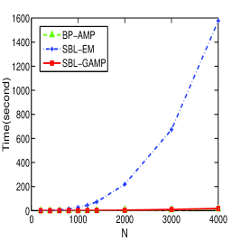
(a)	(b)

Figure 1: (a). Phase transitions of respective algorithms; (b). Average run times vs. $N$.

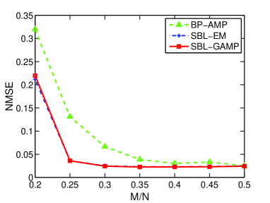
Figure 2: NMSEs of respective algorithms vs. the ratio $M/N$.

We first examine the phase transition behavior of respective algorithms. The phase transition is used to illustrate how sparsity level ($K/M$) and the oversampling ratio ($M/N$) affect the success rate of each algorithm in exactly recovering sparse signals in noiseless scenarios. In particular, each point on the phase transition curve corresponds to a success rate equal to $0.5$. The success rate is computed as the ratio of the number of successful trials to the total number of independent runs. A trial is considered successful if the normalized squared error $\|\boldsymbol{x}-\boldsymbol{\hat{x}}\|_{2}^{2}/\|\boldsymbol{x}\|_{2}^{2}$ is no greater than $10^{-6}$. Fig. 1(a) plots the phase transitions of respective algorithms, where we set $N=1000$, and the oversampling ratio $M/N$ varies from $0.05$ to $0.95$. From Fig. 1(a), we see that, when $M/N<0.5$, the proposed SBL-GAMP algorithm achieves performance similar to SBL-EM, and is superior to BP-AMP. The proposed method is surpassed by BP-AMP as the oversampling ratio increases. Nevertheless, SBL-GAMP is still more appealing since we usually prefer compressed sensing algorithms work under high compression rate regions. The average run times of respective algorithms as a function of the signal dimension $N$ is plotted in Fig. 1(b), where we set $M=0.4N$ and $K=0.3M$. Results are averaged over 10 independent runs. We see that the SBL-GAMP consumes much less time than the SBL-EM due to its easy computation of the posterior distribution of $\boldsymbol{x}$, particularly for a large signal dimension $N$. Also, it can be observed that the average run time of the SBL-EM grows exponentially with $N$, whereas the average run time of the SBL-GAMP grows very slowly with an increasing $N$. This observation coincides with our computational complexity analysis very well. Lastly, we examine the recovery performance in a noisy scenario, where we set $N=500$, $K=40$, and the signal to noise ratio (SNR) is set to 20dB. Fig. 2 depicts the normalized mean square errors (NMSE) of respective algorithms vs. $M/N$. Results are averaged over 1000 independent runs. We see that the SBL-GAMP algorithm achieves a similar recovery accuracy as the SBL-EM algorithm even with a much lower computational complexity.

V Conclusions

We developed a computationally efficient sparse Bayesian learning (SBL) algorithm via the GAMP technique. The proposed method has a much lower computational complexity (of order $\mathcal{O}(MN)$) than the conventional SBL method. Simulation results show that the proposed method achieves recovery performance similar to the conventional SBL method in the low oversampling ratio regime.

References

• [1] J.Β A. Tropp and A.Β C. Gilbert, β€œSignal recovery from random measurements via orthogonal matching pursuit,” IEEE Trans. Information Theory, vol.Β 53, no.Β 12, pp. 4655–4666, Dec. 2007.
• [2] E.Β CandΓ©s and T.Β Tao, β€œDecoding by linear programming,” IEEE Trans. Information Theory, no.Β 12, pp. 4203–4215, Dec. 2005.
• [3] D.Β Wipf and S.Β Nagarajan, β€œIterative reweighted $\ell_{1}$ and $\ell_{2}$ methods for finding sparse solutions,” IEEE Journals of Selected Topics in Signal Processing, vol.Β 4, no.Β 2, pp. 317–329, Apr. 2010.
• [4] M.Β Tipping, β€œSparse Bayesian learning and the relevance vector machine,” Journal of Machine Learning Research, vol.Β 1, pp. 211–244, 2001.
• [5] D.Β P. Wipf, β€œBayesian methods for finding sparse representations,” Ph.D. dissertation, University of California, San Diego, 2006.
• [6] S.Β Ji, Y.Β Xue, and L.Β Carin, β€œBayesian compressive sensing,” IEEE Trans. Signal Processing, vol.Β 56, no.Β 6, pp. 2346–2356, June 2008.
• [7] D.Β L. Donoho, A.Β Maleki, and A.Β Montanari, β€œMessage passing algorithms for compressed sensing,” Proc. Natl. Acad. Sci., vol. 106, pp. 18 914–18 919, Nov. 2009.
• [8] β€”β€”, β€œMessage passing algorithms for compressed sensing: I. motivation and construction,” in Proc. Inf. Theory Workshop, Cairo, Egypt, Jan. 2010.
• [9] S.Β Rangan, β€œGeneralized approximate message passing for estimation with random linear mixing,” in Proc. IEEE Int. Symp. Inf. Theory (ISIT), Saint Petersburg, Russia, Aug. 2011.
• [10] S.Β Som and P.Β Schniter, β€œCompressive imaging using approximate message passing and a Markov-tree prior,” IEEE Trans. Signal Processing, no.Β 7, pp. 3439–3448, July 2012.
• [11] J.Β P. Vila and P.Β Schniter, β€œExpectation-maximization Gaussian-mixture approximate message passing,” IEEE Trans. Signal Processing, no.Β 19, pp. 4658–4672, Oct. 2013.
• [12] X.Β Tan and J.Β Li, β€œComputationally efficient sparse Bayesian learning via belief propagation,” IEEE Trans. Signal Processing, no.Β 4, pp. 2010–2021, Apr. 2010.