An Analytical Window into the World of Ultracold Atoms

Abstract

In this paper, we review the recent developments which had taken place in the domain of quasi one dimensional Bose-Einstein Condensates (BECs) from the viewpoint of integrability. To start with, we consider the dynamics of scalar BECs in a time independent harmonic trap and observe that the scattering length can be suitably manipulated either to compress the bright solitons to attain peak matter wave density without causing their explosion or to broaden the width of the condensates without diluting them. When the harmonic trap frequency becomes time dependent, we notice that one can stabilize the condensates in the confining domain while the density of the condensates continue to increase in the expulsive region. We also observe that the trap frequency and the temporal scattering length can be manoeuvred to generate matter wave interference patterns indicating the coherent nature of the atoms in the condensates. We also notice that a small repulsive three body interaction when reinforced with attractive binary interaction can extend the region of stability of the condensates in the quasi-one dimensional regime.

On the other hand, the investigation of two component BECs in a time dependent harmonic trap suggests that it is possible to switch matter wave energy from one mode to the other confirming the fact that vector BECs are long lived compared to scalar BECs. The Feshbach resonance management of vector BECs indicates that the two component BECs in a time dependent harmonic trap are more stable compared to the condensates in a time independent trap. The introduction of weak (linear) time dependent Rabi coupling rapidly compresses the bright solitons which however can be again stabilized through Feshbach resonance or by finetuning the Rabi coupling while the spatial coupling of vector BECs introduces a phase difference between the condensates which subsequently can be exploited to generate interference pattern in the bright or dark solitons.

I Introduction

We are aware that eventhough matter pervades the entire universe, it is found in just a few admissible forms such as solid, liquid and gas. It is obvious that one can initiate a phase transition between different states of matter by either increasing the temperature or pressure. This understanding of generating new states of matter by increasing the temperature was exploited in 1879 by Sir William Crookes crook79 to create “plasma,” a gas containing non negligible number of charge carriers. It must be mentioned that the physical states of matter change in going from one phase to another while the chemical compositions of matter remains the same. Can one go down the temperature scale and generate a new state of matter at ultra cold temperatures? This question has been plagueing the minds of scientists and it was in 1995, Cornell and Wieman ander95 created a “Bose-Einstein condensate” (BEC) at super low temperatures. Eventhough envisioned first by Albert Einstein and a young Indian physicist named Satyendra Nath Bose in the 1920s einst-einst ; bose24 , it took more than seven decades to realize this singular state of matter. In contrast to plasmas containing superhot and super excited atoms, BECs were created at colder and colder temperatures near absolute zero and they are composed of supercold and super unexcited atoms (see Fig. (1)).

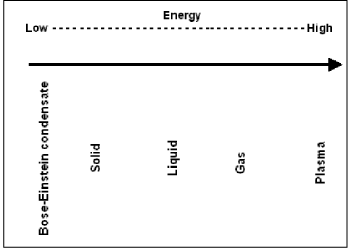
Figure 1: The energy levels of different physical states of matter.

At such low temperatures, a large fraction of the atoms get piled up either in the ground state or in the long lived metastable state. In other words, the atoms merge together losing their individual identities and behave like a giant matter wave. This phenomenon is known as “Bose-Einstein condensation.”

II Gross-Pitaevskii (GP) equation

To investigate the dynamics of a Bose-Einstein condensate, we now employ a Hartree or mean field approach and assume that the wave function is a symmetrized product of single particle wave functions. In the fully condensed state, all bosons (atoms with integral spin) are in the same single-particle state, $\phi(\bf{r})$ and therefore one can write down the wave function of the $N$-particle system as

$$\Psi(\bf{r}_{1},\bf{r}_{2},\ldots,\bf{r}_{N})=\prod_{i=1}^{N}\phi(\bf{r}_{i}).$$ (1)

The single-particle wave function $\phi({\bf r}_{i})$ is normalized as

$$\int d{\bf{r}}|\phi({\bf{r}})|^{2}=1.$$ (2)

This wave function does not contain the correlations produced by the interaction when two atoms are close to each other. These effects are taken into account by using the effective interaction $U_{0}\delta({\bf r}-{\bf r^{\prime}})$. According to mean field theory, the effective Hamiltonian may be written as

$$H=\sum_{i=1}^{N}\left[\frac{{\bf{p}}_{i}^{2}}{2m}+V({\bf{r}}_{i})\right]+U_{0}\sum_{i<j}\delta({\bf{r}}_{i}-{\bf{r}}_{j}),$$ (3)

$V({\bf{r}}_{i})$ being the external potential. The energy of the state given by equation (1) is written as

$$E=N\int d{\bf r}\left[\frac{\hbar^{2}}{2m}|\nabla\phi({\bf r})|^{2}+V({\bf r})|\phi({\bf r})|^{2}+\frac{N-1}{2}U_{0}|\phi({\bf r})|^{4}\right].$$ (4)

From the macroscopic theory for the uniform Bose gas, the relative reduction of the number of particles in the condensate is of the order of $(na^{3})^{1/2}$, where $n$ is the particle density. If we introduce the wave function of the condensed state as

$$\psi({\bf r})=N^{1/2}\phi({\bf r}),$$ (5)

then the density of particles is given by

$$n({\bf r})=|\psi({\bf r})|^{2}$$ (6)

and for $N\gg 1$, the energy of the system may therefore be written as

$$E=\int d{\bf r}\left[\frac{\hbar^{2}}{2m}|\nabla\psi({\bf r})|^{2}+V({\bf r})|\psi({\bf r})|^{2}+\frac{1}{2}U_{0}|\psi({\bf r})|^{4}\right].$$ (7)

To find the optimal form for $\psi$, we minimize the energy with respect to independent variations of $\psi(\bf{r})$ and its complex conjugate $\psi^{*}(\bf{r})$, subject to the condition that the total number of particles

$$N=\int d{\bf r}|\psi({\bf r})|^{2}$$ (8)

be constant. For this, one writes $\delta E-\mu\delta N=0$ where the chemical potential $\mu$ is the Lagrange multiplier that ensures constancy of the particles and the variations of $\psi$ and $\psi^{*}$ may thus be taken to be arbitrary. Equating to zero the variation of $E-\mu N$ with respect to $\psi^{*}(\bf{r})$ gives the following evolution equation gross61 ; gross63 ; pitae61

$$-\frac{\hbar^{2}}{2m}\nabla^{2}\psi({\bf r})+V({\bf r})\psi({\bf r})+U_{0}|\psi({\bf r})|^{2}\psi({\bf r})=\mu\psi({\bf r}).$$ (9)

We call equation (9) as the “time-independent Gross-Pitaevskii equation.” This has the form of a time-independent Schrödinger equation in which the potential acting on particles is the sum of the external potential $V({\bf r})$ and a nonlinear term $U_{0}|\psi({\bf{r}})|^{2}$ that takes into account the mean field produced by the other bosons.

If one has to look for the dynamics of condensates, it is natural to use the time-dependent generalization of the Schrödinger equation with the same nonlinear interaction term and obtain the time-dependent GP equation

$$-\frac{\hbar^{2}}{2m}\nabla^{2}\psi({\bf r})+V({\bf r})\psi({\bf r})+U_{0}|\psi({\bf r})|^{2}\psi({\bf r})=i\hbar\frac{\partial\psi({\bf r},t)}{\partial t}.$$ (10)

To ensure consistency between the time-dependent GP equation (10) and the time-independent GP equation (9), under stationary conditions $\psi({\bf r},t)$ must evolve in time as $\exp(-i\mu t/\hbar)$.

In the above equation (10), $\psi({\bf r},t)$, $r=(x,y,z)$ represents the condensate wave function, $\nabla^{2}$ denotes the Laplacian operator, $V(\bf{r})$ is the trapping potential assumed to be $V({\bf r})=m(\omega_{r}^{2}r^{2}+\omega_{x}^{2}x^{2})$ where $r^{2}=y^{2}+z^{2}$, $\omega_{r,x}$ are the confinement frequencies in the radial and axial directions respectively, $U_{0}=4\pi\hbar^{2}a/m$ corresponds to the strength of interatomic interaction between the atoms characterized by the short-range s-wave scattering length $a$, and $m$ is the atom mass.

From equation (10) it is obvious that the GP equation is an inhomogeneous (3+1) dimensional nonlinear Schrödinger (NLS) equation. The inhomogeneity originates from the potential $V({\bf r})$ that traps the atoms in the ground state and the nonlinearity coefficient $U_{0}$ which represents the interatomic interaction related to the scattering length $a$. The scattering length can have either positive or negative values which means the interaction can be either repulsive or attractive. It should be mentioned that it should be possible to vary the scattering length periodically with time $a(t)$ employing Feshbach resonance inouy98 . This means that understanding the dynamics of BECs boils down to solving a variable coefficient (3+1) NLS equation for suitable choices of trapping potentials $V({\bf{r}})$ and temporal scattering lengths $a(t)$.

III Integrability of GP equation- Review of analytical methods

Looking back at the (3+1) dimensional Gross-Pitaevskii equation (10), it is obvious that it is in general nonintegrable for an arbitrary trapping potential and interatomic interaction. Hence, one has to investigate whether the GP equation would admit integrability in lower spatial dimensions for specific choices of trapping potentials and scattering lengths. In other words, one has to look for the associated nonlinear excitations in (1+1) and (2+1) dimensional GP equations which would reflect upon the integrability of the associated dynamical system under consideration. In a three dimensional BEC, when the transverse trapping frequency $\omega_{r}$ ($r=y,z$) is very high compared to the longitudinal trapping frequency $\omega_{x}$, then the transverse confinement is too tight to allow scattering of atoms to the excited states of the harmonic trap in the transverse direction. Under this condition, one obtains “cigar” shaped BECs and the three dimensional GP equation becomes quasi one-dimensional in nature. Again, it should be mentioned that the quasi one-dimensional GP equation can be shown to be integrable only for suitable choices of trapping potential $V(x)$ and interatomic interaction $U_{0}(x)$.

A. Analytical Methods

Eventhough one cannot precisely define the concept of integrability of a dynamical system governed by a nonlinear partial differential equation (PDE), one can look for the possible signatures of integrability namely, Painleve (P-)property pproperty , Lax-pair lax soliton solutions etc. A given nonlinear dynamical system governed by a nonlinear PDE is said to admit P- property if the corresponding solution can be locally given in terms of a Laurent series expansion in the neighborhood of a movable singular point/manifold. The existence of a Lax-pair of a given nonlinear pde implies that one can somehow linearize the nonlinear dynamical system and subsequently exploit it to generate soliton solutions, thereby consolidating its integrability. In this section, we dwell upon the analytical techniques like Inverse Scattering transform ist , Gauge transformation method llc , Darboux transformation approach darboux ; mateev ; mateev:2 , Hirota’s direct method hblm ; hblm:2 besides the approximation method like variational approach.

I. Inverse Scattering Transform

The Inverse scattering Transform is a nonlinear analogue of the Fourier transform which has been employed to solve several linear partial differential equations. Given the initial value of the potential $q(x,0)$ and the boundary conditions, one has to identify two linear differential operators $L$ and $B$ so that one can convert a (1+1) dimensional nonlinear pde into two linear equations, namely a linear eigenvalue problem

$$L\Phi=\lambda\Phi,$$ (11)

and a linear time evolution equation

$$\Phi_{t}=B\Phi,$$ (12)

such that the compatability condition of the above two equations (11) and (12), i.e., $L_{t}=[B,L]$ generates the nonlinear PDE one has started with. Once the linearization is performed in the above sense for a given nonlinear dispersive system $q_{t}=K(q)$, where $K(q)$ is a nonlinear functional of $q$ and its spatial derivatives, the Cauchy initial value problem corresponding to the boundary condition $q\rightarrow 0$ as $|x|\rightarrow\infty$ can be solved by a three step process indicated schematically in Fig. 2.

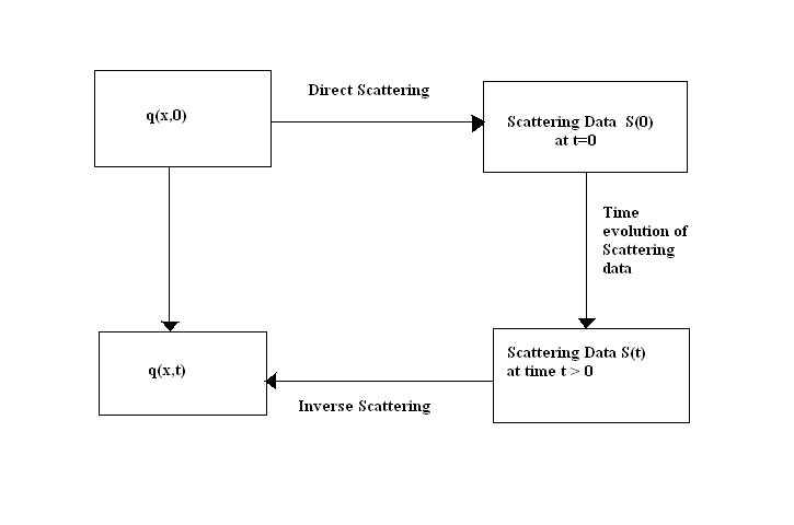
Figure 2: Schematic diagram of the inverse scattering transform method.

This method involves the following three steps:

1. Direct scattering transform analysis

   Considering the initial condition $q(x,0)$ as the potential, an analysis of the linear eigenvalue problem (11) is carried out to obtain the scattering data $S(0)$. For example, for the KdV equation we have

   $$S(0)=\lambda_{n}(0),n=1,2,\ldots,N,C_{n}(0),R(x,0),-\infty<x<\infty$$ (13)

   where $N$ is the number of bound states with eigenvalues $\lambda_{n}$, $C_{n}(0)$ is the normalization constant of the bound state eigenfunctions and $R(x,0)$ is the reflection coefficient for the scattering data.
   

2. Time evolution of scattering data

   Using the asymptotic form of the time evolution equation (12) for the eigenfunctions, the time evolution of the scattering data $S(t)$ can be determined.

3. Inverse scattering transform (IST) analysis

   The set of $Gelfand-Levitan-Marchenko$ integral equations corresponding to the scattering data $S(t)$ is constructed and solved. The resulting solution consists typically of $N$ number of localized, exponentially decaying solutions asymptotically $(t\rightarrow\pm\infty)$. In this way, one can successfully solve the initial value problem of the nonlinear PDE.

From the above, it is obvious that solving the initial value problem of the given nonlinear PDE boils down to solving an integral equation.

II. Gauge Transformation Approach

This is an iterative method enabling one to generate soliton solutions starting from a seed solution. In this method, one again begins with the Zakharov-Shabat(ZS)-Ablowitz-Kaup-Newell-Segur (AKNS) linear systems zakha72 ; ablow73-73 given by the following equations:

$$\Phi_{x}=U\Phi$$ (14)

$$\Phi_{t}=V\Phi$$ (15)

where

$$U=\left(\begin{array}[]{cc}-i\lambda&q\\ r&i\lambda\\ \end{array}\right)\hskip 14.22636pt,\hskip 28.45274ptV=\left(\begin{array}[]{cc}A&B\\ C&D\\ \end{array}\right).$$ (16)

In the above equation, that is equation (16), $\lambda$ represents the spectral parameter, $(q,r)$ the potential/field variable of the given nonlinear PDE, $A,B,C$ and $D$ correspond to the undetermined functions of $\lambda,x,t,q,r$ and their spatial/time derivatives. The compatibility condition ${(\Phi_{x})}_{t}={(\Phi_{t})}_{x}$ yields $U_{t}-V_{x}+[U,V]=$ 0 which is equivalent to the given nonlinear PDE. One generally calls the matrices $U$ and $V$ as “Lax-pair” which contains information about the linearization of the given dynamical system. It should be mentioned that for scalar nonlinear PDEs, $U$ and $V$ are 2$\times$2 matrices and the eigenfunction $\Phi$ is 2$\times$1 column vector while for vector (two component in general) nonlinear PDEs, the eigenfunction $\Phi$ is a 3$\times$1 column vector and $U$ and $V$ are 3$\times$3 matrices.

Now, gauge transforming the eigen function $\Phi$, we have an iterated eigen function $\Phi^{(1)}$=g $\Phi$ where $g$ = $g(x,t,\lambda)$ is a 2$\times$2 matrix function so that

$$\Phi^{(1)}_{x}=U^{(1)}\Phi$$ (17)

$$\Phi^{(1)}_{t}=V^{(1)}\Phi$$ (18)

where,

$$U^{(1)}=gUg^{-1}+g_{x}g^{-1},$$ (19)

$$V^{(1)}=gVg^{-1}+g_{t}g^{-1}.$$ (20)

The transformation function $g$ must be adopted from the solutions of certain Riemann problems in the complex $\lambda$ plane and it must be a meromorphic (regular) function. The simplest form of $g$ satisfying the above criteria can be written as

$$g=\left[I+\frac{\lambda_{1}-\mu_{1}}{\lambda-\lambda_{1}}P(x,t)\right]\left(\begin{array}[]{cc}1&0\\ 0&-1\\ \end{array}\right),$$ (21)

where $\lambda_{1}$ and $\mu_{1}$ are two arbitrary complex numbers and $P$ is an undetermined $2\times 2$ projection matrix $(P^{2}=P)$. Hence, $g^{-1}$ is now given by

$$g^{-1}=\left(\begin{array}[]{cc}1&0\\ 0&-1\\ \end{array}\right)\cdot\left[I-\frac{\lambda_{1}-\mu_{1}}{\lambda-\mu_{1}}P(x,t)\right].$$ (22)

Thus, the vanishing of the apparent residues at $\lambda=\lambda_{1}$ and $\lambda=\mu_{1}$ imposes the following constraints on $P$ as

$$P_{x} = (I-P)\sigma_{3}U(\mu_{1})\sigma_{3}P-P\sigma_{3}U(\lambda_{1})\sigma_{3}(I-P),$$ (23)

$$P_{t} = (I-P)\sigma_{3}V(\mu_{1})\sigma_{3}P-P\sigma_{3}V(\lambda_{1})\sigma_{3}(I-P),$$ (24)

where

$$\sigma_{3}=\left(\begin{array}[]{cc}1&0\\ 0&-1\\ \end{array}\right).$$ (25)

To generate a new solution from a given solution (vacuum), for example $q^{0}$ and $r^{0}$ associated with matrices $U^{0}$ and $V^{0}$, the eigen value problem takes the following form

$$\Phi_{x}^{0}=U^{0}\Phi^{0};\quad\quad\Phi_{t}^{0}=V^{0}\Phi^{0}.$$ (26)

where $U|_{seed}=U^{0}$ and $V|_{seed}=U^{0}$. Now, one can solve equations (23) and (24) using the vacuum eigen function $\Phi^{0}$ such that

$$P=\sigma_{3}\tilde{P}\sigma_{3},$$ (27)

where

$$\tilde{P}=M^{(1)}/[\rm trace\it M^{(\rm 1)}].$$ (28)

and $M^{(1)}$ is a 2$\times$2 matrix defined by

$$M^{(1)}\equiv\Phi^{0}(x,t;\mu_{1})\left(\begin{array}[]{cc}m_{1}&1/n_{1}\\ n_{1}&1/m_{1}\\ \end{array}\right)\Phi^{0}(x,t;\lambda_{1})^{-1},$$ (29)

where $m_{1}$ and $n_{1}$ are arbitrary complex constants and $\Phi^{0}$ is a solution of the vacuum linear system governed by equations (26).

Now, substituting the meromorphic function $g$ with the projection matrix $P$ given by equation (27) into equation (19), we get

$$U^{\prime}(\lambda)=\left(\begin{array}[]{cc}-i\lambda&-q^{0}\\ -r^{0}&i\lambda\\ \end{array}\right)-2i(\lambda_{1}-\mu_{1})\left(\begin{array}[]{cc}0&\tilde{P}_{12}\\ -\tilde{P}_{21}&0\\ \end{array}\right).$$ (30)

A comparison of the eigenvalue problems expressed in terms of the vacuum eigenfunction $\Phi^{0}$ and the new (transformed) eigenfunction $\Phi^{(1)}$ would enable us to relate the vacuum solution of the associated nonlinear PDE with the new solution. Thus, we get an explicit solution as llc

$$q^{(1)}=-q^{0}-2i(\lambda_{1}-\mu_{1})\tilde{P}_{12},$$ (31)

$$r^{(1)}=-r^{0}+2i(\lambda_{1}-\mu_{1})\tilde{P}_{21},$$ (32)

where

$$\tilde{P}_{12}=\frac{M_{12}^{(1)}}{M_{11}^{(1)}+M_{22}^{(1)}},\quad\quad\tilde{P}_{21}=\frac{M_{21}^{(1)}}{M_{11}^{(1)}+M_{22}^{(1)}}.$$ (33)

Once we get $q^{(1)}$ and $r^{(1)}$ from the input solution $q^{0}$ and $r^{0}$, one can repeat the same procedure to obtain yet another new solution $q^{(2)}$ and $r^{(2)}$) using $q^{(1)}$ and $r^{(1)}$) as the input solution. For example, to construct second iterated solution $q^{(2)}$, $r^{(2)}$, one needs to find a solution of the linear system given by equations (17) and (18) where the matrices $U^{1}$ and $V^{1}$ are associated with the input solutions $q^{(1)}$ and $r^{(1)}$. However, one can find the solution of above eigen value problem in terms of $\Phi^{0}$ as

$$\Phi^{(1)}=g\Phi^{0}.$$ (34)

Thus, the new iterated solution $q^{(2)}$ and $r^{(2)}$ (in analogy with equations (31) and (32)) can be written as

$$q^{(2)}=-q^{(1)}-2i(\lambda_{2}-\mu_{2})\tilde{P}_{12}^{(1)},$$ (35)

$$r^{(2)}=-r^{(1)}+2i(\lambda_{2}-\mu_{2})\tilde{P}_{21}^{(1)}.$$ (36)

Thus, one can repeat the same procedure $N$-times to obtain the $N^{\rm{th}}$ iterated solution as

$$q^{N}=-q^{(N-1)}-2i(\lambda_{N}-\mu_{N})\tilde{P}^{(N-1)}_{12},$$ (37)

$$r^{N}=-r^{(N-1)}-2i(\lambda_{N}-\mu_{N})\tilde{P}^{(N-1)}_{21}.$$ (38)

The above iteration could become extremely handy, particularly in the context of the generation of multisoliton solutions as one can obtain $N$-soliton solution from the vacuum eigen function $\Phi^{0}$ of the linear system.

III. Darboux Transformation Approach

In 1882 G. Darboux studied the eigen value problem of the one dimensional Schrödinger equation

$$-\Phi_{xx}-q(x)\Phi=\lambda\Phi,$$ (39)

where $q(x)$ is a potential function and $\lambda$ is a constant spectral parameter. He postulated that if $q(x)$ and $\Phi(x,\lambda)$ are two functions satisfying equation (39) and $f(x)=\Phi(x,\lambda_{0})$ is a solution of equation of (39) for $\lambda=\lambda_{0}$ where $\lambda_{0}$ is a fixed constant, the functions $q^{\prime}$ and $\Phi^{\prime}$ are defined by

$$q^{\prime}=q+2(\ln f)_{xx},\quad\quad\Phi^{\prime}(x,\lambda)=\Phi_{x}(x,\lambda)-\frac{f_{x}}{f}\Phi(x,\lambda),$$ (40)

with

$$-\Phi^{\prime}_{xx}-q^{\prime}\Phi^{\prime}=\lambda\Phi^{\prime}.$$ (41)

From equations (39) and (41), it is obvious that they are of the same form. Therefore, the transformation (40) which converts the functions ($q,\Phi$) to ($q^{\prime},\Phi^{\prime}$) satisfying the same partial differential equation is the original Darboux transformation which is valid for $f\neq 0$.

In this method, one again begins with the ZS-AKNS linear eigen value problem given by equations (14) and (15), where the eigen function $\Phi$ is a 2$\times$2 matrix of the following form

$$\Phi(x,t,\lambda)=\left(\begin{array}[]{cc}\Phi_{11}(x,t,\lambda)&\Phi_{12}(x,t,\lambda)\\ \Phi_{21}(x,t,\lambda)&\Phi_{22}(x,t,\lambda)\\ \end{array}\right).$$ (42)

Now, introducing the Darboux transformation into the known eigen function, we now obtain the transformed eigenfunction as

$$\Phi^{(1)}(x,t,\lambda)=D(x,t,\lambda)\Phi(x,t,\lambda),$$ (43)

where $D(x,t,\lambda)$ is the “Darboux matrix” which is equivalent to $\lambda I-S$. While $I$ is the identity matrix, the matrix $S$ can be generated as

$$S=H\Lambda H^{-1},\quad\rm{det}H\neq 0,$$ (44)

where the matrix $H$ is defined as $H=(h_{1},\ldots,h_{N})$, where $h_{i}$ represents the column solution of the linear eigenvalue problem given by equations (14) and (15), $\Lambda=\rm{diag}(\lambda_{1},\ldots,\lambda_{N})$. The new eigen function $\Phi^{(1)}$ again satisfies equations (17) and (18) and the Darboux matrix $D$ plays the role of the transformation function $g$. Accordingly, we have

$$U^{(1)}=DUD^{-1}+D_{x}D^{-1},$$ (45)

$$V^{(1)}=DUD^{-1}+D_{t}D^{-1}.$$ (46)

To check the form of $U^{(1)}$ given by equation (45), we substitute eqns. (14), (17) into the $x$ derivative of equation(43) to obtain

$$U^{(1)}\Phi^{(1)}=D_{x}\Phi+DU\Phi.$$ (47)

Then, making use of equation (43), one obtains equation (45). Similarly, one can check the form of $V^{(1)}$ given by (46).

Thus, starting from a seed solution $U$ of the given nonlinear pde, one can generate the iterated $U^{(1)}$. This procedure can be repeated to generate multisoliton solutions.

IV. Hirota Bilinear Method

Although the inverse scattering formalism was the first analytical technique that has been developed to solve the initial value problem of nonlinear pdes, it involves sophisticated mathematical concepts like solving an integral equation and hence quite complicated and intricate. Moreover in this method, one should have a prior knowledge of the potential $u(x,t)$ at $t=0$, namely the initial data $u(x,0)$ and the boundary conditions imposed on it. On the other hand, eventhough Darboux and gauge transformation approaches are iterative in nature and are purely algebraic without involving highly complex mathematics, they warrant the identification of the Lax-pair of the associated dynamical system. Hence, it is imperative to look for an alternative method to generate localized solutions (soliton solutions) of nonlinear pdes and in this context, Hirota’s direct method comes to our rescue. In this method, neither does one need any prior information about the potential (or physical field) of the associated nonlinear pde, nor the Lax-pair of the associated dynamical system. This method which has an inbuilt deep algebraic and geometric structure is more elegant and straightforward and can be directly employed to generate soliton solutions of nonlinear pdes.

The salient features of the Hirota method are the following:
i) The given nonlinear partial differential equation has to be converted into a bilinear equation through a transformation which can be identified from the Painlevé analysis. Each term of the bilinear equation has the degree two.

The Hirota bilinear operators are defined as

$$D_{t}^{m}D_{x}^{n}(G\cdot F)=\left(\frac{\partial}{\partial t}-\frac{\partial}{\partial t^{\prime}}\right)^{m}\left(\frac{\partial}{\partial x}-\frac{\partial}{\partial x^{\prime}}\right)^{n}$$

$$G(t,x)F(t^{\prime},x^{\prime})|_{t^{\prime}=t,x^{\prime}=x}.$$

ii) The dependent variables $G$ and $F$ in the bilinear form have to be expanded in the form of a power series in terms of a small parameter $\varepsilon$ as

$$G = \varepsilon g^{(1)}+\varepsilon^{3}g^{(3)}+\varepsilon^{5}g^{(5)}+\cdots,$$ (48)

$$F = 1+\varepsilon^{2}f^{(2)}+\varepsilon^{4}f^{(4)}+\cdots.$$ (49)

iii) After substituting the above functions into the bilinear form and equating different powers of $\varepsilon$, a set of linear pdes can be generated.
iv) Finally, solving the linear pdes, one can generate soliton solutions.

It should be mentioned that the key to the success of the method lies in the identification of the dependent variable transformation as well as in choosing an optimum power series to linearise the given nonlinear pde.

III.1 Approximation method

I. Variational Approach

Variational approach is a qualitative semi-analytical approach. By using the variational approximation, one can study the dynamics of Bose-Einstein condensates described by the mean-field Gross-Pitaevskii equation. For the purpouse of variational analysis, Larangian density is calculated for the corresponding time-dependent Gross-Pitaevskii equation and the effective Lagrangian can be obtained by integrating the initial trial wave function with variational parameters over space. The numerical value of each variational parameter can be obtained from the numerical solution of corresponding Euler-Lagrangian equations.

IV Bright matter wave solitons and their collision in Scalar BECs in certain simple potentials

In this section, we investigate the dynamics of scalar Bose-Einstein condensates in certain simple physically realizable potentials. To start with, we consider the dynamics of BECs in a time independent harmonic trap with exponentially varying scattering length. We generate the associated bright solitons and study their collisional dynamics. We then introduce suitable time dependence in the harmonic trap and investigate the dynamics of BECs. We then show that how the interplay between trap frequency and temporal scattering length can generate matter wave interference pattern in the collision of bright solitons. We then reinforce the binary attraction with a repulsive three body interaction to enhance the stability of BECs.

A. Dynamics of quasi one dimensional BECs in a time independent harmonic trap

For a time independent harmonic oscillator potential and exponentially varying scattering lengths, the GP equation (10) for cigar shaped BECs takes the following form perez98 ; salas02-65 ; liang05 ; khawa06 ; radha07

$$i\frac{{\partial\psi}}{{\partial t}}+\frac{{\partial^{2}\psi}}{{\partial x^{2}}}+2\;a(t)\;\left|{\psi}\right|^{2}\psi+\frac{1}{4}\lambda^{2}x^{2}\psi=0,$$ (50)

where time $t$ and coordinate $x$ are measured in units $2/\omega_{\bot}$ and $a_{\bot}$, where $a_{\bot}=(\hbar/m\omega_{\bot})^{1/2}$ and $a_{0}=(\hbar/m\omega_{0})^{1/2}$ are linear oscillator lengths in the transverse and cigar-axis direction respectively. $\omega_{\bot}$ and $\omega_{0}$ are corresponding harmonic oscillator frequencies, $m$ is the atomic mass and the trap frequency $\lambda=2|\omega_{0}|/\omega_{\bot}<<1$. The Feshbach resonance managed nonlinear coefficient which represents the scattering length reads $a(t)=\tilde{a}_{0}$exp$(\lambda t)$.

Equation (50) admits the following Lax-pair khawa06

$$\Phi_{x} = U\Phi,\;\;\;\;U=\left({\begin{array}[]{*{20}c}{i\zeta}&Q\\ {-Q{*}}&{-i\zeta}\\ \end{array}}\right),$$ (51c)

$$\Phi_{t} = V\Phi,$$ (51d)

$$V = \left({\begin{array}[]{*{20}c}{-2i\zeta^{2}+i\lambda x\zeta+i\left|Q\right|^{2}}&[(\lambda x-2\zeta)Q+iQ_{x}]\\ {[-(\lambda x-2\zeta)Q^{*}+iQ^{*}_{x}]}&{{2i\zeta^{2}-i\lambda x\zeta-i\left|Q\right|^{2}}}\\ \end{array}}\right),$$ (51g)

where we have slightly modified the Lax-pair (given in ref. khawa06 ) by allowing the nonisospectral parameter $\zeta$ to be complex keeping the initial scattering length unity. The nonisospectral complex parameter obeys the first order ordinary differential equation of the form

$$\zeta_{t}=\lambda\zeta,\;\;\;\;\zeta(t)=\alpha(t)+i\beta(t),$$ (52)

and the macroscopic wave function $\psi$ is related to $Q$ by the transformation

$$Q=exp\left(\frac{{\lambda t}}{2}+i\frac{{\lambda x^{2}}}{4}\right)\psi(x,t).$$ (53)

Now, to generate the bright soliton solutions of equation (50), we consider a trivial vacuum solution $Q^{(0)}=0$ to give the following vacuum linear systems

$$\Phi_{x}^{(0)} = \left({\begin{array}[]{*{20}c}{i\zeta}&0\\ {0}&{-i\zeta}\\ \end{array}}\right)\Phi^{(0)}=U^{(0)}\Phi^{(0)},$$ (54c)

$$\Phi_{t}^{(0)} = \left({\begin{array}[]{*{20}c}{-2i\zeta^{2}+i\lambda x\zeta}&0\\ {0}&{{2i\zeta^{2}-i\lambda x\zeta}}\end{array}}\right)\Phi^{(0)}$$ (54f)

$$= V^{(0)}\Phi^{(0)}.$$ (54g)

Solving the above linear systems keeping in mind that the spectral parameter $\zeta$ varies with time by virtue of equation (52), we have

$$\Phi^{(0)}(x,t,\zeta)=\left({\begin{array}[]{*{20}c}{e^{ix\zeta-2i\int\zeta^{2}dt}}&0\\ {0}&{{e^{-ix\zeta+2i\int\zeta^{2}dt}}}\\ \end{array}}\right).$$ (55)

Now, effecting the gauge transformation

$$\Phi^{(1)}(x,t,\zeta)=g\Phi^{(0)}(x,t,\zeta),$$ (56)

where “$g$” is a meromorphic solution of the associated Riemann problem. The new linear eigenvalue problems now take the following form

$$\Phi_{x}^{(1)}=U^{(1)}\Phi^{(1)},\;\;\;\;\Phi_{t}^{(1)}=V^{(1)}\Phi^{(1)},$$ (57)

with

$$U^{(1)}=gU^{(0)}g^{-1}+g_{x}g^{-1},$$ (58a)

$$V^{(1)}=gV^{(0)}g^{-1}+g_{t}g^{-1}.$$ (58b)

We now choose $g$ as

$$g=\left(1+\frac{{\zeta_{1}-\mu_{1}}}{\zeta-\zeta_{1}}P_{1}(x,t)\right)\left({\begin{array}[]{*{20}c}{1}&0\\ {0}&{-1}\\ \end{array}}\right)$$ (59)

where $\zeta_{1}$ and $\mu_{1}$ are arbitrary complex parameters and $P_{1}$ is a projection matrix $(P_{1}^{2}=P_{1})$. Imposing the constraint that $U^{(1)}$ and $V^{(1)}$ do not develop singularities around the poles $\zeta=\zeta_{1}$ and $\zeta=\mu_{1}$, the choice of the projection matrix $P_{1}$ is governed by the solution of the following set of partial differential equations

$$P_{1x} = (1-P_{1})\sigma_{3}U^{(0)}(\mu_{1})\sigma_{3}P_{1}-P_{1}\sigma_{3}U^{(0)}(\zeta_{1})$$ (60a)

$$\sigma_{3}(1-P_{1})$$

$$P_{1t} = (1-P_{1})\sigma_{3}V^{(0)}(\mu_{1})\sigma_{3}P_{1}-P_{1}\sigma_{3}V^{(0)}(\zeta_{1})$$ (60b)

$$\sigma_{3}(1-P_{1})$$

where

$$\sigma_{3}=\left({\begin{array}[]{*{20}c}1&0\\ 0&-1\\ \end{array}}\right).$$ (61)

Looking at the above system of equations, we understand that $P_{1}$ depends only on the trivial matrix eigenfunction $\Phi^{(0)}(x,t,\zeta)$, a diagonal matrix and has a compact form given by

$$P_{1}(x,t) = \sigma_{3}\frac{{M^{(1)}}}{[\rm trace\;M^{(1)}]}\sigma_{3},$$ (62a)

$$M^{(1)} = \left({\begin{array}[]{*{20}c}m_{1}&1/n_{1}\\ n_{1}&{1/m_{1}}\\ \end{array}}\right)\Phi^{(0)}(x,t,\zeta_{1})^{-1}$$ (62d)

where $m_{1}$ and $n_{1}$ are arbitrary complex constants. Hence, choosing the complex parameters $\zeta_{1}=\alpha_{1}(t)+i\beta_{1}(t)$ and $\mu_{1}=\zeta_{1}^{*}$ and employing the gauge transformation approach llc , we arrive at the matter wave bright soliton

$$\psi^{(1)}(x,t)=2\beta_{0}exp\left(\frac{{\lambda t}}{2}-\frac{{i\lambda x^{2}}}{4}\right)sech(\theta_{1})exp(i\xi_{1}),$$ (63)

where

$$\theta_{1} = 2\beta_{1}x-8\int(\alpha_{1}\beta_{1})dt+2\delta_{1},$$ (64a)

$$\xi_{1} = 2\alpha_{1}x-4\int(\alpha_{1}^{2}-\beta_{1}^{2})dt-2\phi_{1},$$ (64b)

$$\alpha_{1} = \alpha_{10}e^{\lambda t},\;\;\;\;\beta_{1}=\beta_{10}e^{\lambda t}.$$ (64c)

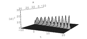
Figure 3: The dynamics of bright solitons for the parametric choice $\lambda$= 0.02, $\beta_{0}$=2, $\alpha_{0}$=0.1, $\delta_{1}$=0.5, $\phi_{1}$=0.1.

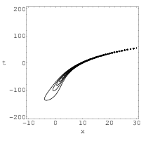
Figure 4: Contour Plot of bright soliton for $\lambda$=0.02.

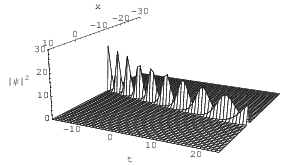
Figure 5: The dynamics of bright soliton for $\lambda$= -0.02.

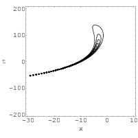
Figure 6: Contour plot of bright soliton for $\lambda$= -0.02.

The above bright soliton solution given by equations (63) and (64a-64c) is identical to the one given by Liang et al. liang05 using Darboux transformation. From the profile of the bright soliton trains shown in Fig. 3, we infer that matter wave density $|\psi|^{2}$ increases with the increase of the absolute value of the scattering length leading to the compression of the bright soliton trains of BEC. The contour plot (shown in Fig. 4) which takes a cross-sectional view of Fig. 3 in the $x-t$ plane shows that the width of bright solitons decreases progressively. Figure 5 shows that the peak value of the matter wave density $|\psi|^{2}$ decreases with the decrease of the absolute value of the scattering length leading to a broadening of the bright soliton trains thereby enhancing their width and this is again confirmed by the corresponding contour plot in figure 6. Our investigation shows that the scattering length can be suitably manipulated to compress the bright solitons of BECs into an assumed peak matter density without causing their explosion while on the other hand, it can be manoeuvred judiciously to broaden the localized solitons without allowing the dilution of the condensates and this interpretation completely agrees with that of Liang et al. liang05 . Investigations of the quasi one dimensional GP equation khawa06 ; liang05 ; chong07 ; li06 ; kengn06 ; yuce07 ; wu07 in the presence of an expulsive parabolic potential for positive scattering lengths also confirm our above observations.

From the above, we observe that one can either compress or broaden the bright solitons in the expulsive time independent trap either by exponentially increasing or decreasing the scattering lengths respectively. It must be mentioned that the exponentially varying scattering length with a trap frequency dependence would make the exact solutions of the GP equation less interesting from an experimental point of view. Hence, it would be interesting to investigate the impact of a general time dependent scattering length and a time dependent trap on the condensates. The addition of time dependent trap frequency will facilitate us to tune the trap suitably and study its impact on the condensates.

B. Impact of transient trap on BECs

The introduction of time dependance in the trap ensures that the condensates are now confronted with both time dependent scattering length and time dependent trapping potential and accordingly equation (50) gets modified as (in dimensionless units) atre06

$$i\frac{\partial\psi}{\partial t}+\frac{1}{2}\frac{\partial^{2}\psi}{\partial x^{2}}+a(t)|\psi|^{2}\psi-\frac{\lambda(t)}{2}x^{2}\psi=0,$$ (65)

where $a(t)=-2a_{s}(t)/a_{B}$, $\lambda(t)=\omega_{0}^{2}(t)/\omega^{2}_{\perp}$, $a_{B}$ is the Bohr radius, $\lambda(t)$ describes time dependent harmonic trap which can be confining ($\lambda(t)<0$) or expulsive ($\lambda(t)>0$). This equation has been mapped onto a linear Schr$\rm\ddot{o}$dinger eigenvalue problem atre06 and one soliton solution has been expressed in terms of doubly periodic Jacobian elliptic functions. However, the above approach cannot be employed to generate multisoliton solutions analytically. The gauge transformation approach comes in handy at this juncture as it offers the advantage of constructing multisoliton solution from the solution of the corresponding vacuum linear system.

Now, to generate the bright solitons of equation (65) for both regular and expulsive potentials, we introduce the following modified lens transformation atre06 ; theoc03-67 ; sulem99 ; wu07

$$\psi(x,t)=\sqrt{A(t)}Q(x,t)\rm exp(i\Phi(x,t)),$$ (66)

where the phase has the following simple quadratic form

$$\Phi(x,t)=-\frac{1}{2}c(t)x^{2}.$$ (67)

Substituting the modified lens transformation given by equation (66) in equation (65), we obtain the modified NLS equation

$$iQ_{t}+\frac{1}{2}Q_{xx}-ic(t)xQ_{x}-ic(t)Q+a(t)A(t)|Q|^{2}Q=0,$$ (68)

with

$$\lambda(t)=c^{\prime}(t)-c(t)^{2},$$ (69)

and

$$c(t)=-\frac{d}{dt}\rm lnA(t).$$ (70)

Equation (68) admits the following linear eigenvalue problem

$$\phi_{x} = U\phi,\qquad U=\left(\begin{array}[]{cc}i\zeta(t)&Q\\ -Q^{*}&-i\zeta(t)\\ \end{array}\right),$$ (73)

$$\phi_{t} = V\phi,$$ (74)

$$V = \left(\begin{array}[]{cc}V_{11}&V_{12}\\ \\ V_{21}&V_{22}\\ \end{array}\right).$$ (78)

where

$$V_{11} = -i\zeta(t)^{2}+ic(t)x\zeta(t)+\frac{i}{2}a(t)A(t)|Q|^{2}$$

$$V_{12} = (c(t)x-\zeta(t))Q+\frac{i}{2}Q_{x}$$

$$V_{21} = -(c(t)x-\zeta(t))Q^{*}+\frac{i}{2}Q^{*}_{x}$$

$$V_{22} = i\zeta(t)^{2}-ic(t)x\zeta(t)-\frac{i}{2}a(t)A(t)|Q|^{2}$$ (79)

In the above linear eigenvalue problem, the spectral parameter “$\zeta$” which is complex is nonisospectral obeying the following equation

$$\zeta^{\prime}(t)=c(t)\zeta(t),$$ (80)

with $a(t)=1/A(t)$. It is obvious that the compatability condition $(\phi_{x})_{t}=(\phi_{t})_{x}$ generates equation (68).

Substituting equation (70) with $a(t)=1/A(t)$ in equation (69), we get

$$a^{\prime\prime}(t)a(t)-2a^{\prime}(t)^{2}-\lambda(t)a(t)^{2}=0.$$ (81)

From the above, it is evident that the GP equation (65) is completely integrable only if the trap frequency $\lambda(t)$ and the scattering length $a(t)$ are connected by equation (81) and the above condition is consistent with Ref. wu07 . Thus, the modified lens transformation has facilitated the identification of integrability of equation (65). It should also be mentioned that equation (65) is completely integrable only for certain suitable choices of trap frequency $\lambda(t)$ depending on the solvability of equation (69). For example, when $\lambda(t)={\rm{constant}}=k$ and $a(t)$=$e^{\Lambda t}$, where $\Lambda$ is the trap frequency, equation (65) reduces to (50) describing the dynamics of BECs moving in an expulsive parabolic potential and exponentially varying scattering length liang05 ; radha07 . The above parametric choice is consistent with equation (81) with $k=-\lambda^{2}$ ensuring the integrability of the model. The above model has also been experimentally realized khayko .

To generate the soliton solution of equation (68) (or equation (65)), we consider the seed solution $Q^{(0)}=0$ and solve the linear systems given by equations (73) and (74) keeping in mind equation (80) to obtain

$$\phi^{(0)}(x,t,\zeta)=\left(\begin{array}[]{cc}e^{ix\zeta(t)-i\int^{t}_{0}\zeta(t)^{2}dt}&0\\ 0&e^{-ix\zeta(t)+i\int^{t}_{0}\zeta(t)^{2}dt}\\ \end{array}\right).$$ (82)

Employing the gauge transformation approach and choosing $\zeta_{1}=\alpha_{1}(t)+i\beta_{1}(t)$ and $\mu_{1}=\zeta_{1}^{*}$, one obtains the one soliton solution of equation (65) rames08pra

$$\psi^{1}(x,t)=\sqrt{\frac{1}{a(t)}}2\beta_{1}(t)\;\;\rm{sech}\theta_{1}\;\;e^{-\frac{i}{2}c(t)x^{2}+i\xi_{1}},$$ (83)

where

$$\theta_{1} = 2\beta_{1}(t)x-4\int^{t}_{0}{(\alpha_{1}(t^{{}^{\prime}})\beta_{1}(t^{{}^{\prime}}))}dt^{{}^{\prime}}+2\delta_{1},$$

$$\xi_{1} = 2\alpha_{1}(t)x-2\int^{t}_{0}{(\alpha_{1}(t^{{}^{\prime}})^{2}-\beta_{1}(t^{{}^{\prime}})^{2})}dt^{{}^{\prime}}-2\phi_{1},$$ (84)

$$\alpha_{1} = \alpha_{10}e^{\int^{t}_{0}c(t^{{}^{\prime}})dt^{{}^{\prime}}},$$

$$\beta_{1} = \beta_{10}e^{\int^{t}_{0}c(t^{{}^{\prime}})dt^{{}^{\prime}}},$$

and $\phi_{1}$, $\delta_{1}$, $\alpha_{10}$ and $\beta_{10}$ are arbitrary real constants.

The striking feature of this bright soliton solution is that its amplitude relies strongly on the scattering length $a(t)$ and the time dependent trap $\lambda(t)$ while the velocity is governed by the external trap $\lambda(t)$ alone.

This procedure can be easily extended to generate multisoliton solution and one can study the collisional dynamics of bright solitons for a suitable choice of $\lambda(t)$ and $a(t)$ consistent with equation (81).

Thus, it is obvious that one can obtain varieties of soliton profiles depending on the choice of the scattering length $a(t)$ and the time dependent trap $\lambda(t)$ consistent with equation (81).

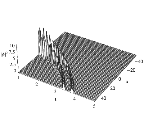
Figure 7: Two soliton interaction in the expulsive trap ($\lambda(t)<0$) with $a(t)$ =$a_{0}exp(-0.125t^{2})$, $a_{0}=0.5$, $\alpha_{10}=2.31$, $\beta_{10}=1.5$, $\alpha_{20}=3.12$, $\beta_{20}=1.2$, $\phi_{1}=.005$, $\delta_{1}=0.002$, $\phi_{2}=0.002$, $\delta_{2}=0.001$.

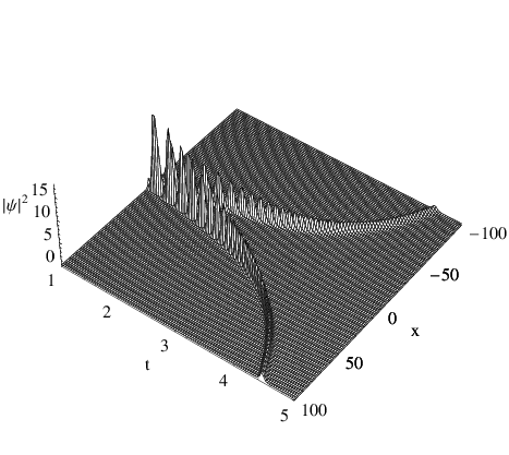
Figure 8: Two soliton interaction in the expulsive trap ($\lambda(t)<0$) with $a(t)$ =$a_{0}exp(-0.125t^{2})$, $a_{0}=0.5$, $\alpha_{10}=2.31$, $\beta_{10}=1.5$, $\alpha_{20}=-2.12$, $\beta_{20}=1.2$, $\phi_{1}=.05$, $\delta_{1}=0.02$, $\phi_{2}=0.02$, $\delta_{2}=0.01$.

Figures (7) and (8) describe the evolution of the two soliton solution for an expulsive trap ($\lambda(t)<0$) for different initial conditions evolving the scattering length of the form $a(t)=0.5\exp(-0.125t^{2})$. From the figures, one observes that the matter wave density $|\psi|^{2}$ of the condensates decreases slowly by virtue of the decrease in the absolute value of the scattering length and the trajectory of the soliton pulses is dictated by the initial conditions. It should be mentioned that the identification of this critical parametric regime in which one observes the slow decay of the condensates enables one to avoid this domain by operating the system under a safe range of parameters.

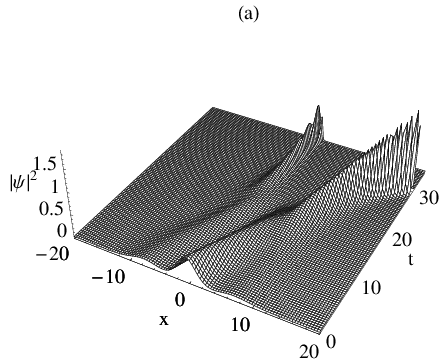
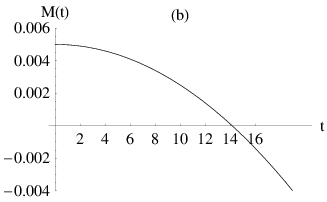
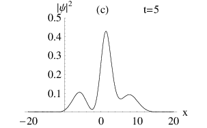
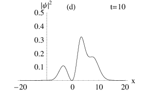
Figure 9: Two soliton interaction in the confining trap ($\lambda(t)>0$) at different intervals of time with $a(t)$ =$a_{0}$ $\exp(0.0025t^{2})$, $a_{0}=0.5$, $\alpha_{10}=0.01$, $\beta_{10}=0.1$, $\alpha_{20}=0.28$, $\beta_{20}=0.11$, $\phi_{1}=\delta_{2}=0.1$, $\phi_{2}=\delta_{1}=0.2$.

Figure 9 (a) shows the interaction of solitons for $a(t)=0.5\exp(0.0025t^{2})$. It can be observed from fig. (9b) that the confining nature of the trap ($\lambda(t)>0$) is preserved only for a finite length of time ($t<14$). During this period, the two soliton pulses slide over each other like liquid balls as shown in figures 9 (c) and 9 (d). After this critical period ($t>$14), the trap becomes expulsive again which sets in the compression of the soliton pulses resulting in the increase of the matter wave density $|\psi|^{2}$ of the condensates. It can also be observed that for $a(t)=0.5\exp(-0.125t^{2})$, the absolute value of the scattering length decreases and hence there is a slow decay of the condensates while for $a(t)=0.5\exp(0.0025t^{2})$, eventhough the absolute value of the scattering length increases, the soliton pulses begin to get compressed (or the matter wave density $|\psi|^{2}$ increases) after a finite time delay. It can be easily understood that this delay is introduced by the time dependent trap. When the time dependent trap $\lambda(t)$ becomes a constant, equation (65) reduces to the dynamics of BECs in an expulsive parabolic potential and time independent scattering length. Under this condition, the soliton trains begin getting compressed and the matter wave density $|\psi|^{2}$ increases as soon as the absolute value of the scattering length increases and one does not observe any time delay in the compression of soliton trains liang05 ; radha07 . It should also be mentioned that this time delay in the compression of the soliton pulses can be suitably manipulated by changing the trapping coefficient $\lambda(t)$. Thus, the bright solitons can be compressed into a desired width and amplitude in a controlled manner by suitably changing the trap and our observation is consistent with the numerical results xue05 .

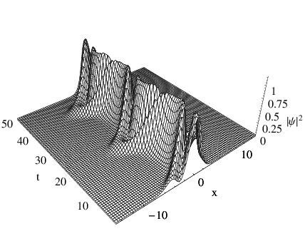
Figure 10: Two soliton interaction in the confining trap ($\lambda(t)=0.09$) with $a(t)$ =$a_{0}$ $\exp(0.3it)$, $a_{0}=0.5$, $\alpha_{10}=0.09$, $\beta_{10}=0.71$, $\alpha_{20}=0.031$, $\beta_{20}=0.11$, $\phi_{1}=5.1$, $\delta_{1}=7.2$, $\phi_{2}=4.2$, $\delta_{2}=4.1$.

It can also be observed that at $t>$14, the time dependent trap becomes expulsive again for the same choice of $a(t)$ (i.e., $a(t)=0.5\exp(0.0025t^{2})$) (fig. 9b). In order to sustain the confining nature of the trap ($\lambda(t)>$0), the scattering length should become complex as it is being done in the case of cold alkaline earth metal atoms ciury05 . Under this condition, the matter wave density $|\psi|^{2}$ periodically changes with time by virtue of the periodic modulation of scattering length kevre03 ; pelin03 and this is reminiscent of the recent experimental observation of Faraday waves engel07 . We also observe that the two soliton pulses keep exchanging energy among themselves continuously during propagation as shown in Fig. 10

We observe from the above that the addition of time dependence in the trap enables one to stabilize the condensates for a longer period of time by selectively tuning the trapping potential. It should be mentioned that one can also selectively choose $\lambda(t)$ and a(t) and observe their interplay in the collisional dynamics of bright solitons. The interplay between $\lambda(t)$ and a(t) consistent with equation (81) results in the “matter-wave interference pattern” in the collisional dynamics of bright solitons.

C. Matter wave interference pattern in the collision of bright solitons

To generate the matter wave interference pattern, we now allow the two bright solitons to collide with each other in the presence of a trap for suitable choices of scattering length $a(t)$ and trap frequency $\lambda(t)$ (or $c(t)$) consistent with equation (81).

Case (i): When $c(t)=-1$, the scattering length evolves as $a(t)=a_{0}e^{-t}$ (shown in Fig. 12(b)) where $a_{0}$ is an arbitrary real constant and the trap frequency $\lambda(t)$ becomes expulsive and is equal to a constant ($\lambda(t)=-1$). Under this condition, the collisional dynamics of two bright solitons which are initially separated as shown in Fig. 11 (a) in the expulsive harmonic trap is shown in Fig. 11 (b) and the corresponding density evolution in Fig. 12 (a). The density evolution consists of alternating bright and dark fringes of high and low density respectively while the phase difference between the condensates continuously changes with time as shown in Fig. 14 (a).

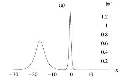
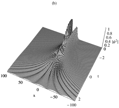
Figure 11: (a) Initial position of two bright solitons at $t=-3$ for $c(t)=-1$. (b) Interaction of two bright solitons forming the interference pattern for the choice $a(t)=a_{0}e^{-t}$ with $\alpha_{10}$=0.01, $\alpha_{20}$=0.8, $\beta_{10}$=0.06, $\beta_{20}$=0.012, $a_{0}$=0.2, $\phi_{1}$ =0.01, $\phi_{2}$=0.1, $\delta_{1}$=0.1, $\delta_{2}$=0.01.

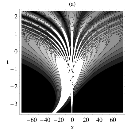
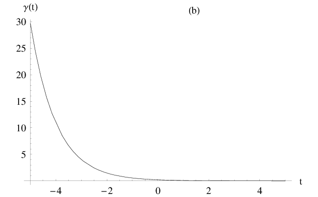
Figure 12: (a)Contour plot of fig.11(b) depicting matter wave density evolution, (b) The time evolution of scattering length $a(t)$ corresponding to case (i).

Case(ii): When $\lambda(t)=0.3-0.09t^{2}$ (shown in Fig. 13(a)) and $a(t)=a_{0}e^{(0.15t^{2})}$, the soliton interaction and the corresponding contour plot showing the interference pattern in the confining region are shown in Figs. 13 (b) and 13 (c) respectively. From the Figs. 13 (a)-(c), it is clear that when the trap $\lambda(t)$ enters the confining region from the expulsive domain, the interaction of the solitons generates the interference pattern in the confining regime and the pattern disappears once the trap becomes expulsive again. The above choice of $\lambda(t)$ and $a(t)$ can be synthesized easily under suitable laboratory conditions. The phase difference between the condensates continuously changes with time as shown in Fig. 14 (b)

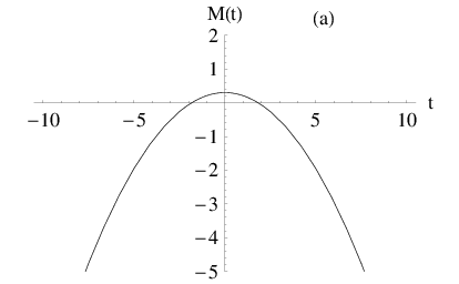
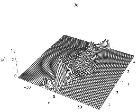
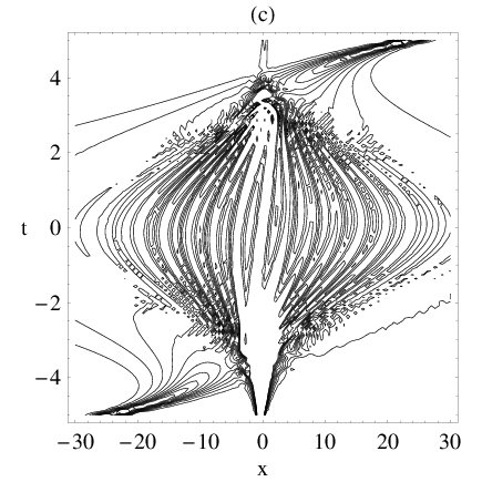
Figure 13: (a) The time evolution of the trap $\lambda(t)=0.3-0.09t^{2}$ corresponding to case (ii), (b) Two soliton interaction forming the interference pattern corresponding to case (ii) for the choice $a(t)=a_{0}e^{(0.15t^{2})}$ with $\alpha_{10}$=0.01, $\alpha_{20}$=0.8, $\beta_{10}$=0.06, $\beta_{20}$=0.012, $a_{0}$=0.02, $\phi_{1}$ =0.2, $\phi_{2}$=0.1, $\delta_{1}$=0.1, $\delta_{2}$=0.2, (c) Contour plot showing the interference pattern in the confining regime.

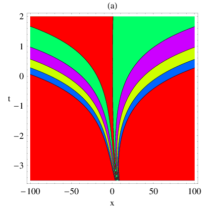
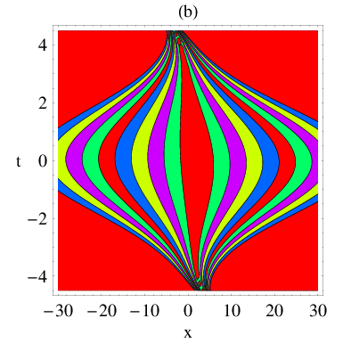
Figure 14: (a) The phase difference between the condensates corresponding to case (i) and (b) case (ii).

Thus, our results reinforce the fact that the matter waves originating from the condensates (bright solitons) do interfere and produce a fringe pattern analogous to the coherent laser beams and the interference pattern is a clear signature of the long range spatial coherence of the condensates. The interference pattern generated by virtue of the collision of two bright solitons rames09pla is analogous to the interference pattern obtained earlier experimentally by Andrews et al. andre97 wherein the two condensates were separated with a sheet of green light and overlapped in ballistic expansion (switching off the trap) while we selectively tune the frequency of the trap $\lambda(t)$ in accordance with the scattering length $a(t)$ consistent with equation (81). These interference patterns are completely different from the interference of two independent condensates originating from two different traps with or without phase javan96 ; javan86 ; javan91 .

It should be mentioned that the optical traps have opened up the possibility of realizing different types of temporal variation of the trap frequency $\lambda(t)$ while the scattering length can be controlled both by Feshbach resonance as well as through the trap frequency $\lambda(t)$. The phase change evolution shown in Figs. 14 (a) and 14 (b) gives a measure of the coherence of the condensates. It must be added that though the concept of coherence of matter waves was already exploited to create atom lasers, we do reconfirm the coherent nature of BECs in the intra trap collision of bright solitons.

D. Dynamics of BECs with two and three body interactions

In equation (50), when the scattering length exponentially increases with time via Feshbach resoncance, the density of the condensates also increases liang05 ; radha07 . Naturally, a question arises as to how far one can increase the scattering length to produce high density condensates. Since collapse of the condensates sets in once the density exceeds a critical value and one does not expect the collapse of BECs for a true one-dimensional system, there is a constraint on increasing the density of the condensates to sustain an effective true one-dimensional BEC liang05 . This implies that one has to investigate the dynamics of BECs within a safe range of parameters. Hence, one has to look for an alternative to generate high density condensates retaining the one-dimensionality of the system without restricting to a parametric domain. It was observed that for a large number of bosons, the repulsive three-body interactions can overcome the two-body attractive interactions thereby enhancing the stability of the condensates nref14 .

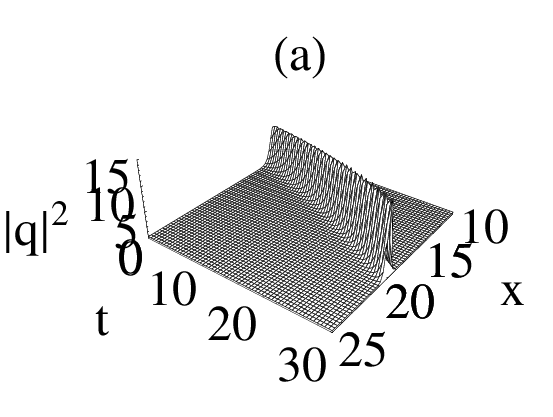
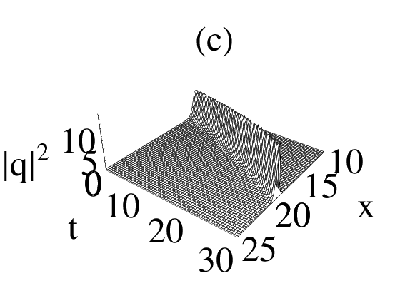
Figure 15: Density of condensates in the modified GP equation with both attractive two-body and attractive three-body interactions for the parametric choice $\lambda$=0.02, $\alpha_{0}$=0.1, $\beta_{0}$=0.9, $\delta_{1}$=$-$1.5, $\phi_{1}$=2.5 for (a) $\tilde{a}_{0}$=0.4, $\tau=0$, (b)$\tilde{a}_{0}$=0.4, $\tau=0.04$, (c)$\tilde{a}_{0}$=0.45, $\tau=0.04$.

From the above, we understand that two-body interactions alone are insufficient and they have to be suitably combined with three-body interactions to extend the region of stability while increasing the density of the condensates in a quasi one-dimensional regime.

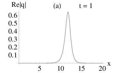
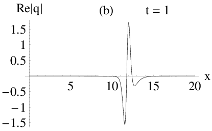
Figure 16: Real part of the order parameter of (a) cubic GP equation and (b) modified GP equation with attractive three-body interactions.

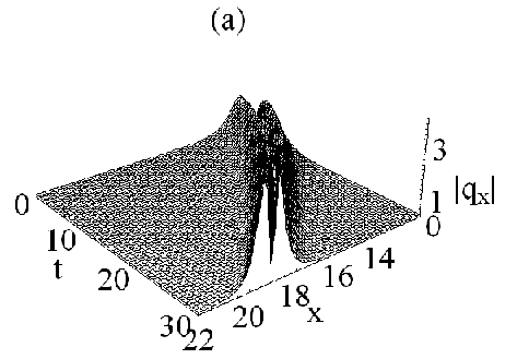
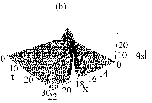
Figure 17: (a) Compression and splitting of $|q_{x}|$ of cubic GP equation (b) Compression and suppression of splitting of $|q_{x}|$ in the modified GP equation.

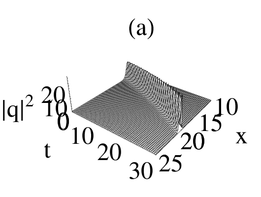
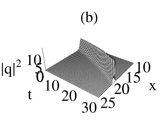
Figure 18: Density of condensates in the modified GP equation with attractive two-body interactions and repulsive three-body interactions with the same parametric choice as in fig.15 for (a) $\tilde{a}_{0}$=0.6, $\bar{\tau}=0.04$, (b)$\tilde{a}_{0}$=0.8, $\bar{\tau}=0.04$, (c)$\tilde{a}_{0}$=0.8, $\bar{\tau}=0.09$.

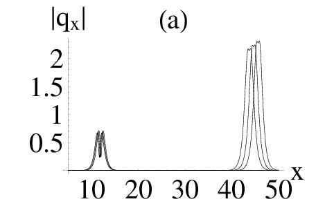
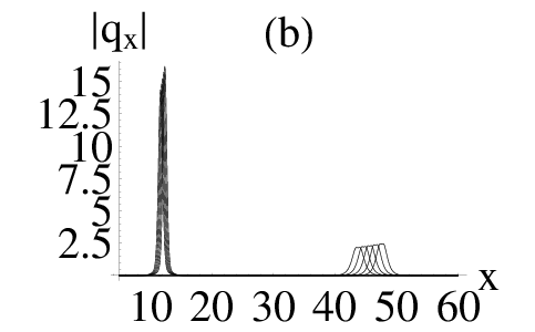
Figure 19: Asymptotic forms of the density profiles $|q_{x}|$ of the two-soliton solution of (a) cubic GP equation and (b) modified GP equation (attractive).

To introduce the new integrable model describing the impact of both two- and three-body interactions on the condensates, we now consider an additional phase imprint on the order parameter $\psi(x,t)$ to generate a new order parameter $q(x,t)$ as

$$q(x,t)=\psi(x,t)\rm{e}^{2i\theta(x,t)},$$ (85)

where $\theta(x,t)$ is the phase-imprint on the old order parameter $\psi(x,t)$. We now engineer the phase imprint $\theta(x,t)$ in accordance with the following equations;

$$\theta_{x}=-\sqrt{\tau}|\psi|^{2},$$ (86)

$$\theta_{t}=i\sqrt{\tau}(\psi\psi^{*}_{x}-\psi^{*}\psi_{x})+4\tau|\psi|^{4},$$ (87)

so that the transformed order parameter $q(x,t)$ obeys an evolution equation

$$iq_{t}+q_{xx}+2a(t)|q|^{2}q+\frac{\lambda^{2}x^{2}}{4}q+4\tau|q|^{4}q+4i\sqrt{\tau}(|q|^{2})_{x}q=0.$$ (88)

In equation(88), $a(t)(=\tilde{a}_{0}$exp$(\lambda t)$) represents attractive ($\tilde{a}_{0}>0$) two-body interactions while the real and arbitrary parameter $\tau$ corresponds to the strength of three-body interactions assuming that the contribution of three-atom collisions to the loss is negligible (by kicking out atoms from the condensate into thermal cloud) nref14 -nref19 . This type of engineering the phase imprint to generate a new integrable model describing the impact of both two- and three-body interactions on the condensates is reminiscent of generating solitons by phase engineering of BECs of sodium and rubidium nref22 .

Making use of the gauge transformation approach, we obtain the bright one soliton solution of the modified GP equation (88)jpsj

$$q^{(1)}=\frac{2}{\sqrt{\tilde{a}_{0}}}\beta_{0}\rm{e}^{\left(\frac{{\lambda t}}{2}-\frac{{i\lambda x^{2}}}{4}+2i\theta\right)}\rm{sech}(\chi_{1})\rm{exp}(i\xi_{1}),$$ (89)

$$\chi_{1} = 2\beta_{1}x-8\int(\alpha_{1}\beta_{1})dt+2\delta_{1},$$ (90)

$$\xi_{1} = 2\alpha_{1}x-4\int(\alpha_{1}^{2}-\beta_{1}^{2})dt-2\phi_{1},$$ (91)

$$\alpha_{1} = \alpha_{0}\rm{e}^{\lambda t},\;\;\;\;\beta_{1}=\beta_{0}\rm{e}^{\lambda t},$$ (92)

and

$$\theta=-\frac{2}{\tilde{a}_{0}}\sqrt{\tau}\beta_{0}\rm{tanh}\left[2\left(\frac{\rm{e}^{\lambda t}(x\lambda-2\rm{e}^{\lambda t}\alpha_{0})\beta_{0}}{\lambda}+\delta_{1}\right)\right],$$ (93)

where $\alpha_{0}$, $\beta_{0}$, $\delta_{1}$ and $\phi_{1}$ are arbitrary real constants. It should be mentioned that the phase imprint $\theta$ given by equation (93) is related to the density of the old order parameter $\psi$ (by virtue of equations (86) and (87) and hence the bright solitons given by equation(89) are endowed with phase dependent amplitude. It should also be added that equation (88) admits bright solitons only for attractive two-body interactions ($\tilde{a}_{0}>0$) while the three-body interactions can be either attractive ($\tau>0$) or repulsive ($\tau<0$).

I. Condensates with attractive three-body interactions ($\tau>0$)

From the equations (89)-(93), one observes that the bright solitons of the integrable modified GP equation (88) acquires a kink like additional nontrivial phase represented by equation (93) in comparison with that of cubic GP solitons ($\tau=0$). Figure 15 (a) portrays the density evolution of the condensates in the absence of three-body interactions. When one considers the attractive three-body interactions in addition to the attractive two-body interactions with the strength of both being equal, one does not observe any perceptible change in the matter wave density as shown in Fig. 15 (b). When the strength of attractive two-body interactions is increased, one observes a decrease in the density of condensates as shown in Fig. 15 (c). From this, one understands that an instability sets in the condensates leading to the ejection of the atoms resulting in the decrease of matter wave density. Hence, to ensure the stability of the condensates over a longer interval of time, the strength of the attractive two-body interactions should be minimum.

It is also obvious that this additional phase arising in the dynamics of the condensates of the modified GP equation with attractive three-body interactions evolves in space and time as indicated by equation (93) and hence one understands that its effect will be more pronounced either in the real (or imaginary) part or in the derivatives of the order parameter. Figure 16 (b) shows the effect of the nontrivial phase on the matter wave solitons of the modified GP equation in comparison with that of cubic GP equation shown in Fig. 16 (a). Thus, it is evident that the additional nontrivial phase contributes to the compression and rarefaction of the matter wave solitons of the modified GP equation.

From the spatial derivative $|q_{x}|$ plotted in Figs. 17 (a) and 17 (b), one infers that as the atoms start accumulating in the lowest quantum state, the matter wave density increases leading to a compression of the matter wave of the cubic GP equation. In addition to the compression, there is a splitting of the matter wave in the cubic GP equation (see Fig. 17 (a)), while this splitting of the matter wave has been completely suppressed by the attractive three-body interactions as shown in Fig. 17 (b).

II. Condensates with repulsive three-body interactions ($\tau<0$)

For repulsive three-body interactions, the bright soliton of integrable modified GP equation becomes

$$\bar{q}^{(1)}=\frac{2}{\sqrt{\tilde{a}_{0}}}\beta_{0}\rm{sech}(\chi_{1})\rm{exp}(i\xi_{1})\rm{e}^{\left(\frac{{\lambda t}}{2}-\frac{{i\lambda x^{2}}}{4}+\bar{\theta}\right)},$$ (94)

where $\bar{\theta}=\frac{4}{\tilde{a}_{0}}\sqrt{\bar{\tau}}\beta_{0}\rm{tanh}\left[2\left(\frac{\rm{e}^{\lambda t}(x\lambda-2\rm{e}^{\lambda t}\alpha_{0})\beta_{0}}{\lambda}+\delta_{1}\right)\right]$ with $\bar{\tau}$ being a real parameter.

   Figure 18 (a) displays the density evolution of the condensates for attractive two-body interactions and repulsive three-body interactions. Thus, the addition of a small repulsive three-body force contributes to an exponential increase in the matter wave density (as the amplitude of the condensates becomes $\frac{2}{\sqrt{\tilde{a}_{0}}}\beta_{0}\rm{exp}(\lambda t/2+\bar{\theta})$ from equation (94) in comparison to the density evolution of the condensates in the absence of three-body interactions shown in Fig .15(a). The fact that the condensates can hold enormous number of atoms together with a small repulsive force means that one can extend the region of stability of the condensates in a quasi one-dimensional regime. When one increases the strength of attractive two-body interactions, the density of the condensates decreases as shown in Fig. 18 (b) as compared to Fig. 18 (a), thereby setting in an instability in the condensates. However, this instability can be overcome by increasing the strength of repulsive three-body interactions as shown in Fig. 18 (c), wherein the matter wave density again increases enormously in comparison with Fig. 18 (b) and attains the magnitude shown in Fig. 18 (a). Thus, we observe that the addition of repulsive three-body interactions can allow the number of condensed atoms to increase enormously and this can happen even when the strength of the repulsive three-body interactions is very small compared with the strength of two-body interactionsnref14 . It should be mentioned that eventhough the bright solitons of the modified GP equation with both two- and three-body interactions (both repulsive and attractive) in the expulsive potential are unstable again, the extent of instability has reduced compared to that of a cubic GP equation with two-body interactions alone.

V Dynamics of Vector Bose-Einstein Condensates

We know that the behaviour of single component (or scalar) BECs is influenced by the external trapping potential and interatomic interaction. Experimental realization of BECs in which two (or more) internal states or different atoms can be populated has given a fillip to the investigation of multicomponent BECs ho96 ; esry97 ; pu98 . In contrast to the single component BECs, the behaviour of multicomponent condensates is much richer because of both intra species interaction and inter species interaction. This extra freedom arising by virtue of the interaction among the internal states or different atoms offers multicomponent BECs several interesting and complicated properties which are not witnessed in single component condensates. Far from being a trivial extension of the single component BECs, multicomponent condensates exhibit novel and rich phenomena such as soliton trains, soliton pairs, multidomain walls, spin-switching ieda04 ; uchiy06 and multimode collective excitations.

Motivated by the above considerations, we investigate the dynamics of a two-component BEC in a time dependent harmonic trap described by a two-coupled GP equation and deduce the integrability condition for the existence of vector bright solitons. We then bring out the fascinating collision of vector bright solitons demonstrating the switching of energy underscoring the longevity of vector BECs. We then employ Feshbach resonance management to manoeuvre the scattering length to further enhance the lifetime of two component BECs.

A. Mathematical Model

Considering a two-component BEC, the behaviour of the condensates that are prepared in two hyperfine states can be described at sufficiently low temperatures by the two coupled GP equation of the following form ho96 ; esry97 ; pu98

$$i\hbar\frac{\partial\psi_{1}}{\partial t}=\left(-\frac{\hbar^{2}}{2m_{1}}\nabla^{2}+U_{11}|\psi_{1}|^{2}+U_{12}|\psi_{2}|^{2}+V_{1}\right)\psi_{1},$$ (95)

$$i\hbar\frac{\partial\psi_{2}}{\partial t}=\left(-\frac{\hbar^{2}}{2m_{2}}\nabla^{2}+U_{21}|\psi_{1}|^{2}+U_{22}|\psi_{2}|^{2}+V_{2}\right)\psi_{2},$$ (96)

where the condensate wave functions are normalized through the particle numbers $N_{i}=\int|\psi_{i}|^{2}d^{3}{\textbf{r}}$. $U_{ii}=4\pi\hbar^{2}a_{ii}/m$ and $U_{ij}=2\pi\hbar^{2}a_{ij}/m$ represent intraspecies and interspecies interaction strengths respectively with $a_{ij}$ being the corresponding scattering lengths and $m$ is the reduced mass. The trapping potentials are assumed to be $V_{i}=m_{i}[\omega_{ix}^{2}x^{2}+\omega_{i\bot}^{2}(y^{2}+z^{2})]/2$. Further assuming that $\omega_{i\bot}\gg\omega_{ix}$ such that the transverse motions of the condensates are frozen to the ground state of the transverse harmonic trapping potential, the system becomes quasi one dimensional in nature. Integrating out the transverse coordinates, the resulting equations for the axial wave functions $\psi_{1,2}(x,t)$ in dimensionless form can be written as

$$i\frac{\partial\psi_{1}}{\partial t}=\left(-\frac{1}{2}\frac{\partial^{2}}{\partial x^{2}}+b_{11}|\psi_{1}|^{2}+b_{12}|\psi_{2}|^{2}+\frac{\lambda_{1}^{2}}{2}x^{2}\right)\psi_{1},$$ (97)

$$i\frac{\partial\psi_{2}}{\partial t}=\left(-\frac{k}{2}\frac{\partial^{2}}{\partial x^{2}}+b_{21}|\psi_{1}|^{2}+b_{22}|\psi_{2}|^{2}+\frac{\lambda_{2}^{2}}{2k}x^{2}\right)\psi_{2},$$ (98)

where units for length and time become $\sqrt{\frac{\hbar}{m_{1}\omega_{1\bot}}}$ and $2\pi/\omega_{1\bot}$ and $\psi_{1,2}$ is normalized such that $\int|\psi_{1}|^{2}dx=1$ and $\int|\psi_{2}|^{2}dx=N_{2}/N_{1}$. Other parameters are defined as: $b_{11}=2a_{11}N_{1}$, $b_{12}=2m_{1}a_{12}N_{1}/[(1+\omega_{2\bot}/\omega_{1\bot})m]$, $b_{21}=2m_{1}a_{21}N_{1}/[(1+\omega_{2\bot}/\omega_{1\bot})m]$, $b_{22}=2a_{22}kN_{1}\omega_{2\bot}/\omega_{1\bot}$, $\lambda_{1}=\omega_{1x}/\omega_{1\bot}$, $\lambda_{2}=\omega_{2x}/\omega_{1\bot}$ and $k=m_{1}/m_{2}$.

Now, we consider $k=1$ (i.e., $m_{1}=m_{2}$) and $\omega_{1}=\omega_{2}=\omega$ (i.e., $\lambda_{1}=\lambda_{2}$) and allow the scattering lengths $a_{ij}$ and the strength of trapping potential $\lambda^{2}(\lambda=\omega_{x}/\omega_{\bot})$ to vary with time. Then, the above equation with $\tilde{t}=t/2$ takes the following form (after omitting tilde)

$$i\psi_{1t}+\psi_{1xx}+2(b_{11}(t)|\psi_{1}|^{2}+b_{12}(t)|\psi_{2}|^{2})\psi_{1}+\lambda(t)^{2}x^{2}\psi_{1}=0,$$ (99)

$$i\psi_{2t}+\psi_{2xx}+2(b_{21}(t)|\psi_{1}|^{2}+b_{22}(t)|\psi_{2}|^{2})\psi_{2}+\lambda(t)^{2}x^{2}\psi_{2}=0,$$ (100)

In the above equation, $b_{ij}(i,j=1,2)$ represents the attractive interaction strength and the trap frequency could be both confining ($\lambda(t)^{2}>0$) and expulsive ($\lambda(t)^{2}<0$). When the longitudinal trapping potential is neglected ($\lambda(t)$=0) and $b_{11}=b_{12}=b_{21}=b_{22}=\rm{a~{}constant}$, the system becomes the celebrated Manakov model (see Refs. makha81 to liu09 ) admitting shape changing collision of vector solitons.

When both intraspecies interaction and interspecies interaction are all equal and time dependent (i.e., $b_{11}(t)=b_{12}(t)=b_{21}(t)=b_{22}(t)=a(t)$), the above equations (99) and (100) take the following form

$$i\psi_{1t}+\psi_{1xx}+2a(t)(|\psi_{1}|^{2}+|\psi_{2}|^{2})\psi_{1}+\lambda(t)^{2}x^{2}\psi_{1}=0,$$ (101)

$$i\psi_{2t}+\psi_{2xx}+2a(t)(|\psi_{1}|^{2}+|\psi_{2}|^{2})\psi_{2}+\lambda(t)^{2}x^{2}\psi_{2}=0,$$ (102)

The above coupled GP equation has been investigated and shown to admit integrability for symmetric interaction strengths liu09 ; zhang09 ; rajen09 .

B. Lax-pair and integrability condition

Equations (101) and (102) admit the following linear eigenvalue problem

$$\Phi_{x} + U\Phi=0,$$ (103)

$$\Phi_{t} + V\Phi=0,$$ (104)

where $\Phi=(\phi_{1},\phi_{2},\phi_{3})^{T}$ and

$$U = \left(\begin{array}[]{ccc}i\zeta(t)&Q_{1}&Q_{2}\\ Q_{1}^{*}&-i\zeta(t)&0\\ Q_{2}^{*}&0&-i\zeta(t)\\ \end{array}\right),$$ (108)

$$V = \left(\begin{array}[]{ccc}V_{11}&V_{12}&V_{13}\\ V_{21}&V_{22}&V_{23}\\ V_{31}&V_{32}&V_{33}\\ \end{array}\right),$$ (112)

with

$$v_{11} = -i\zeta(t)^{2}+i\Gamma(t)x\zeta(t)+\frac{i}{2}Q_{1}Q_{1}^{*}+\frac{i}{2}Q_{2}Q_{2}^{*}$$

$$v_{12} = (\Gamma(t)x-\zeta(t))Q_{1}+\frac{i}{2}Q_{1x}$$

$$v_{13} = (\Gamma(t)x-\zeta(t))Q_{2}+\frac{i}{2}Q_{2x}$$

$$v_{21} = -(\Gamma(t)x-\zeta(t))Q_{1}^{*}+\frac{i}{2}Q_{1x}^{*}$$

$$v_{22} = i\zeta(t)^{2}-i\Gamma(t)x\zeta(t)-\frac{i}{2}Q_{1}Q_{1}^{*}$$

$$v_{23} = -\frac{i}{2}Q_{2}Q_{1}^{*}$$

$$v_{31} = -(\Gamma(t)x-\zeta(t))Q_{2}^{*}+\frac{i}{2}Q_{1x}^{*}$$

$$v_{32} = -\frac{i}{2}Q_{1}Q_{2}^{*}$$

$$v_{33} = i\zeta(t)^{2}-i\Gamma(t)x\zeta(t)-\frac{i}{2}Q_{2}Q_{2}^{*}$$

$$Q_{1}=\frac{1}{\sqrt{A(t)}}\psi_{1}(x,t)e^{i\Gamma(t)x^{2}}$$

$$Q_{2}=\frac{1}{\sqrt{A(t)}}\psi_{2}(x,t)e^{i\Gamma(t)x^{2}}$$

It is obvious that the compatibility condition $(\Phi_{x})_{t}$=$(\Phi_{t})_{x}$ leads to the zero curvature equation $U_{t}-V_{x}+[U,V]=0$ which yields the integrable coupled GP equation (101) and (102) provided the spectral parameter $\zeta(t)$ obeys the following nonisospectral condition

$$\zeta(t)=\mu e^{-(\int\Gamma(t)dt)}$$ (114)

where $\mu$ is a hidden complex constant and $\Gamma(t)$ is an arbitrary function of time and is related to the trap frequency

$$\lambda^{2}(t)=\Gamma^{2}(t)-\Gamma^{\prime}(t).$$ (115)

Further, equation (115) which represents the trap frequency $\lambda(t)$ can be related to the scattering length $a(t)$ through the integrability condition

$$-a^{\prime\prime}(t)a(t)+2a^{\prime}(t)^{2}-\lambda^{2}(t)a^{2}(t)=0.$$ (116)

It should be mentioned that the coupled GP equation represented by (101) and (102) is completely integrable for suitable choices of the trap frequency $\lambda(t)$ and scattering length $a(t)$ consistent with equation (116). For the constant trapping frequency, $\lambda(t)=c_{1}$, equation (116) yields $a(t)=e^{c_{1}t}$.

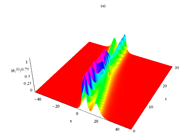
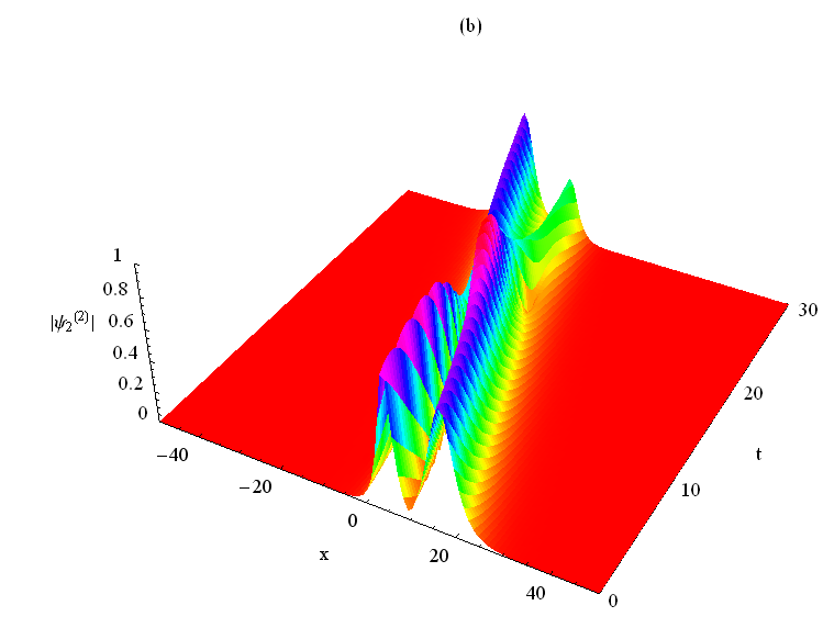
Figure 20: Switching of matter wave (bright) solitons in two component BECs for $a(t)$=0.01 and $\lambda(t)$= 0.01+0.0001 $t^{2}$

The bright solitons of equations (101)-(102) employing gauge transformation method have the following form

$$\psi_{1}^{(1)}=\sqrt{\frac{1}{a(t)}}\varepsilon_{1}^{(1)}2\beta_{1}(t)sech(\theta_{1})e^{i(-\xi_{1}+\Gamma(t)\frac{x^{2}}{2})},$$ (117)

$$\psi_{2}^{(1)}=\sqrt{\frac{1}{a(t)}}\varepsilon_{2}^{(1)}2\beta_{1}(t)sech(\theta_{1})e^{i(-\xi_{1}+\Gamma(t)\frac{x^{2}}{2})},$$ (118)

where

$$\theta_{1} = 4\int\alpha_{1}\beta_{1}dt+2x\beta_{1}-2\delta_{1},$$ (119)

$$\xi_{1} = 2\int(\alpha_{1}^{2}-\beta_{1}^{2})dt+2x\alpha_{1}-2\chi_{1},$$ (120)

with $\alpha_{1}=\alpha_{10}e^{[\int{\Gamma(t)}dt]}$, $\beta_{1}=\beta_{10}e^{[\int{\Gamma(t)}dt]}$ while $\delta_{1}$ and $\chi_{1}$ are arbitrary parameters. Gauge transformation approach can also be extended to generate multi soliton solution twosol.vr.2010 . Figure 20 shows that it should be possible to transfer (switch) energy from one mode to the other in a vector BEC thereby one can enhance the longevity (or lifetime) of the bright solitons (or the condensates). This can happen irrespective of whether the trap is time dependent or independent.

C. Feshbach Resonance Management of vector bright solitonsmypapertobe

It is obvious from the investigation of vector BECs that the lifetime of the condensates gets enhanced by virtue of the switching of energy between the two components. It should be mentioned that Feshbach resonance management can also be employed to drive home the fact that vector BECs in a time dependent harmonic trap are longlived compared to the condensates dwelling in a time independent trap.

To start with, we now switch off the time dependence of the harmonic trap and keep track of the evolution of the condensates by manipulating the scattering length of the form $a(t)=0.5e^{-0.25t}$ (shown in Fig. 21 (f)) consistent with equations (115) and (116), thereby rendering ($\Gamma(t)=-0.25$) the trap expulsive (shown in Fig. 21 (e)). The corresponding density profile of the condensates is shown in the upper panel of Fig. 21 (Figs. 21 (a) and 21 (b)). The associated numerically simulated density profile of the condensates employing real time propagation of Split Step Crank Nicolson method is shown in Figs. 21 (c) and 21 (d). From Figs. 21 (a)-21 (d), we observe that there is a perfect agreement between analytical and numerical results. When we double the trap frequency ($\Gamma(t)=-0.5$) keeping the trap expulsive again (shown in Fig. 22 (e)) and manipulate the scattering length through Feshbach resonance of the form $a(t)=0.5e^{-0.5t}$ (shown in Fig. 22 (f)) consistent with equations(115) and (116), the compression (analytical) the condensates sets in the two modes as shown in Figs. 22 (a)-(b). This is again confirmed by the numerical simulation shown in Figs. 22 (c) and 22 (d). When we further enhance the trap strength (3.6 times the original strength) keeping the trap expulsive again (shown in Fig. 23 (e)) and further manipulate scattering length a(t) of the form $a(t)=0.5e^{-0.9t}$ (shown in Fig. 23(f)), one observes the onset of collapse of the condensates as shown in Figs. 23 (a)-(b). Again, the numerically simulated condensates shown in Figs. 23 (c) and 23 (d) match with Figs. 23 (a) and 23 (b) respectively.

To enhance the stability of the condensates, we now switch on the time dependence in the harmonic trap keeping it expulsive (shown in Fig. 24 (e)) of the form $\Gamma(t)=-0.25t$ and manipulate the scattering length through Feshbach resonance of the form $a(t)=0.5e^{-0.125t^{2}}$ shown in Fig. 24 (f) consistent with equations (115) and (116), the corresponding density profile is shown in Figs.24 (a)-(b). This is confirmed by the numerical simulation of the condensates shown in Figs. 24 (c) and 24 (d). When we make a 20 fold increase in the expulsive trap frequency (shown in Fig. 25 (e)) and accordingly employ Feshbach resonance to choose $a(t)=0.5e^{-2.5t^{2}}$ (shown in Fig. 25 (f)) consistent with equations (115) and (116), the corresponding density profile shown in Figs. 25(a)-(b) exactly match with the numerically simulated condensates in Figs. 25 (c) and 25 (d).

When we further enhance the time dependent expulsive trap (shown in Fig. 26 (e)) frequency $\Gamma(t)$ by 100 times the original strength and manipulate scattering length (shown in Fig. 26 (f)) through Feshbach resonance (in accordance with equations (115 and 116)), one never sees an abrupt increase in the density of the condensates as shown in Figs. 26 (a)-(b). Thus, we observe that any further increase of the expulsive trap frequency $\Gamma(t)$ and manipulation of scattering length through Feshbach resonance does not significantly increase the density of the condensates eventhough the attractive interaction strength increases rapidly. In other words, the condensates in the time dependent expulsive harmonic trap continue to remain stable for a reasonably large interval of time even for large attractive interactions. Again, analytical results synchronize with numerical simulations shown in Figs. 26(c)-(d).

Thus, we observe that the vector BECs in a time dependent expulsive trap are more long lived and the lifetime can be enhanced by Feshbach resonance management compared to the condensates in a time independent expulsive harmonic trap. We also wish to point out that we are able to stabilize the condensates in an expulsive time dependent harmonic trap for attractive interactions, where the condensates usually get compressed and collapse subsequently. It is also pretty obvious that the scalar counterpart of the condensates stabilized through Feshbach resonance (shown in Figs. 24-26) will collapse immediately during time evolution.

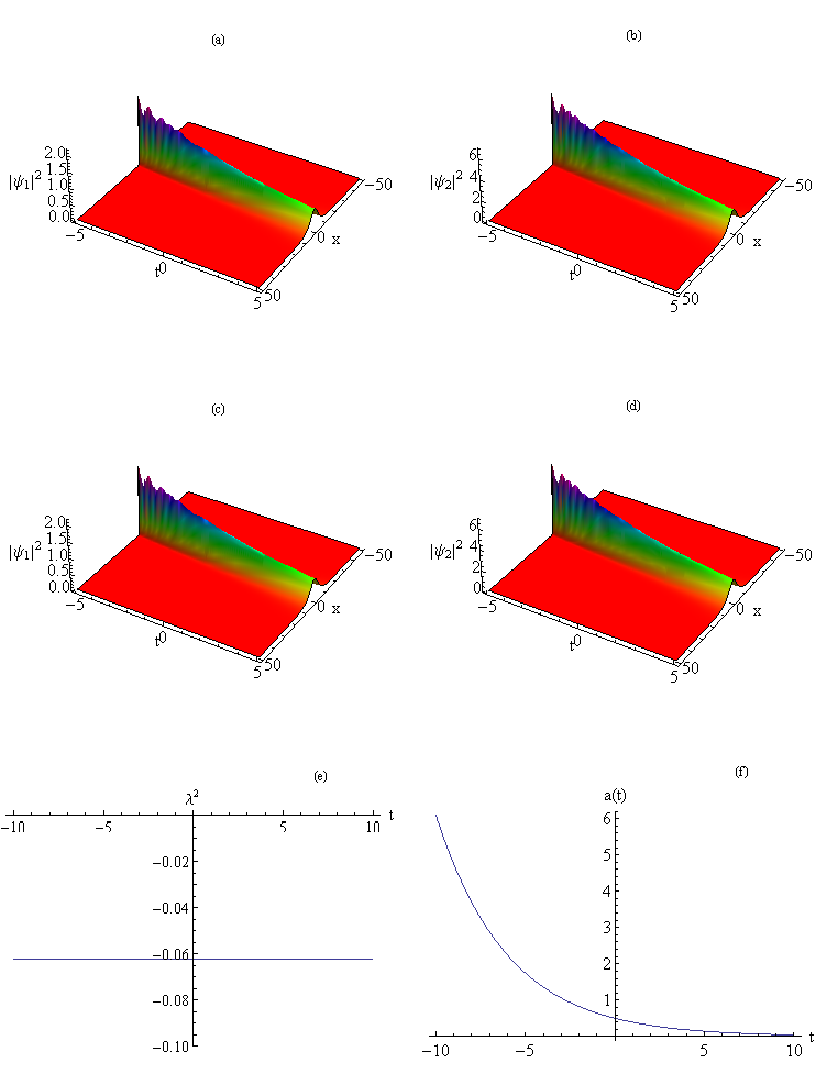
Figure 21: Upper Panel (a)-(b): Density (Analytical) profile of the condensates (bright solitons) in the time independent expulsive trap for $\Gamma(t)$= -0.25 and $a(t)=0.5e^{-0.25t}$; Middle Panel (c)-(d): Numerically simulated density profile for $\Gamma(t)$= -0.25 and $a(t)=0.5e^{-0.25t}$; Lower panel(e)-(f): Trap strength and binary interaction

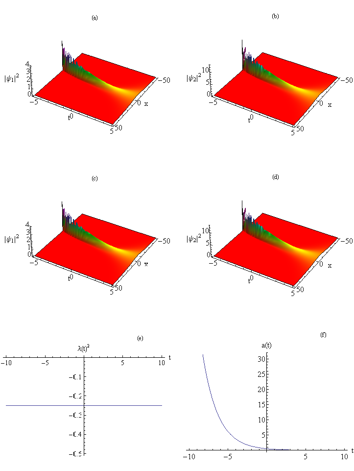
Figure 22: Upper panel (a)-(b): Compression (Analytical) of the condensates in the time independent expulsive trap for $\Gamma(t)$= -0.5 and $a(t)=0.5e^{-0.5t}$; Middle Panel (c)-(d): Numerically simulated density profile for $\Gamma(t)$= -0.5 and $a(t)=0.5e^{-0.5t}$ showing the compression of BECs; Lower panel (e)-(f): Trap strength and binary interaction.

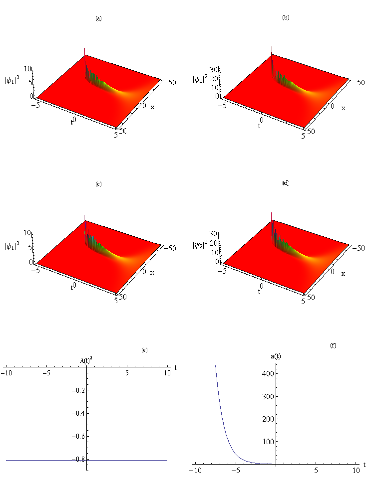
Figure 23: Upper panel (a)-(b): Onset of collapse (Analytical) of the condensates for $\Gamma(t)$= -0.9 and $a(t)=0.5e^{-0.9t}$ in an expulsive time independent trap; Middle Panel (c)-(d): Numerically simulated density profile for $\Gamma(t)$= -0.9 and $a(t)=0.5e^{-0.9t}$ showing the collapse of BECs; Lower panel (e)-(f): Trap strength and binary interaction

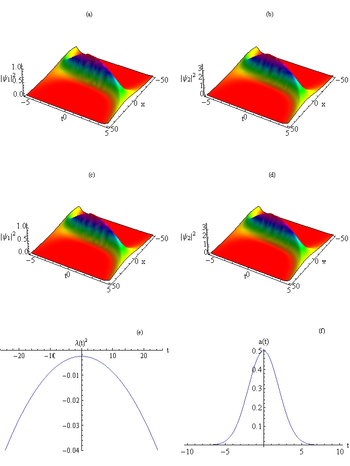
Figure 24: Upper panel (a)-(b): Density (Analytical) profile of the condensates by switching ON the time dependence in the expulsive trap for $\Gamma(t)$=-0.25 t and $a(t)=0.5e^{-0.125t^{2}}$; Middle Panel (c)-(d): Numerically simulated density profile for $\Gamma(t)$=-0.25 t and $a(t)=0.5e^{-0.125t^{2}}$; Lower panel (e)-(f): Transient trap and Interaction strength

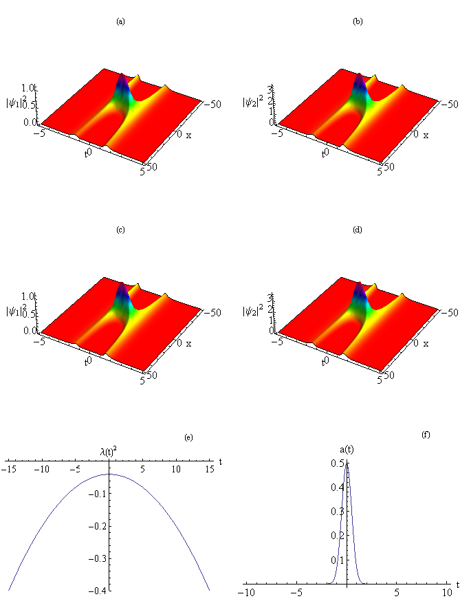
Figure 25: Upper panel (a)-(b):Density (Analytical) profile of the condensates in the time dependent expulsive trap for $\Gamma(t)$=-5 t and $a(t)$=$0.5e^{-2.5t^{2}}$; Middle Panel (c)-(d): Numerically simulated density profile for $\Gamma(t)$=-5 t and $a(t)$=$0.5e^{-2.5t^{2}}$; Lower panel (e)-(f): Transient trap and Interaction strength

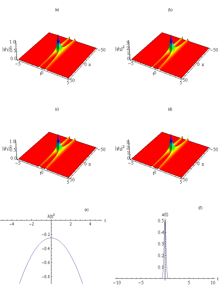
Figure 26: Upper panel (a)-(b): Density (Analytical) profile of the condensates in the time dependent expulsive trap for $\Gamma(t)$=-25 t and $a(t)=0.5e^{-12.5t^{2}}$; Middle Panel (c)-(d): Numerically simulated density profile for $\Gamma(t)$=-25 t and $a(t)=0.5e^{-12.5t^{2}}$; Lower panel (e)-(f): Transient trap and Interaction strength

VI Stabilization of bright solitons in weakly coupled BECs

A. Impact of weak time dependent Rabi coupling

We also emphasize that the enhancement in the lifetime of the two component BECs arises by virtue of intraspecies and interspecies interaction. It should be mentioned that one can make two component BECs more longlived by the addition of weak time dependent or space dependent coupling forces.

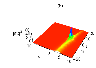
Figure 27: Density of the condensates for $a(t)=0.5t$, $\varepsilon_{1}^{(1)}=0.3$ and $\Gamma(t)=0.1t$ X $10^{-2}$ without coupling.

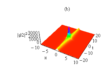
Figure 28: Impact of weak coupling on the condensates with $\nu(t)=0.1t$ with the other parameters as in Fig.27

We now consider a spinor BEC composed of two hyperfine states, say of the $|F=1,m_{f}=-1>$ and $|F=1,m_{f}=1>$ states of ⁸⁷Rb atoms rbatom confined at different vertical positions by parabolic traps and coupled by a time dependent coupling field.

We assume the condensate to be quasi-one-dimensional (cigar-shaped). Then, in the meanfield approximation, the system is described by the coupled GP equation pethick

$$i\psi_{1t}+\psi_{1xx} + 2a(t)(|\psi_{1}|^{2}+|\psi_{2}|^{2})\psi_{1}+\lambda(t)^{2}x^{2}\psi_{1}$$ (121)

$$+ iG(t)\psi_{1}+\nu(t)\psi_{2}=0,$$

$$i\psi_{2t}+\psi_{2xx} + 2a(t)(|\psi_{1}|^{2}+|\psi_{2}|^{2})\psi_{2}+\lambda(t)^{2}x^{2}\psi_{2}$$ (122)

$$+ iG(t)\psi_{2}+\nu(t)\psi_{1}=0,$$

In the above equation, $\nu(t)$ denotes the coupling between the two condensates while $G(t)$ accounts for the feeding (loss/gain) of the condensates from the thermal cloud. Infact, the impact of adding a linear coupling to the Manakov model was already demonstrated ref15 and the resulting dynamical system was shown be integrable. The linearly coupled GP equations (122) have also been investigated and the concept of domain walls ref16 and symmetry breaking of solitons ref17 was explored. Equations (122) have also been investigated for $\nu(t)=0$ rajen09 ; twosol.vr.2010 and the dynamics of vector BECs has been analyzed.

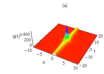
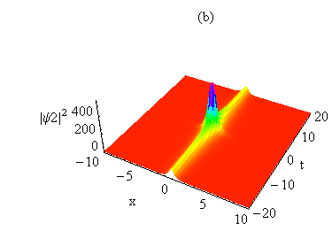
Figure 29: Stabilization of the condensates by tuning the scattering length for $a(t)=0.5$ X $1/2t$ with the other parameters as in Fig. 28

The explicit forms of one soliton solution of equations (122) can be written as ref37

$$\psi_{1}^{(}1)=\frac{2}{\sqrt{a}(t)}\varepsilon_{1}^{(1)}\beta_{1}(t)sech(\theta_{1})e^{i(-\xi_{1}+\Gamma(t)\frac{x^{2}}{2})},$$ (123)

$$\psi_{2}^{(}1)=\frac{2}{\sqrt{a}(t)}\varepsilon_{2}^{(1)}\beta_{1}(t)sech(\theta_{1})e^{i(-\xi_{1}+\Gamma(t)\frac{x^{2}}{2})},$$ (124)

where

$$\theta_{1} = 8\int\alpha_{1}(t)\beta_{1}(t)dt+2x\beta_{1}(t)-2\delta_{1},$$ (125)

$$\xi_{1} = 4\int(\alpha_{1}(t)^{2}-\beta_{1}(t)^{2})dt+2x\alpha_{1}(t)-2\chi_{1},$$ (126)

with $\alpha_{1}(t)=\alpha_{10}e^{-\int 2\Gamma(t)^{2}dt}$, $\beta_{1}(t)=\beta_{10}e^{-\int 2\Gamma(t)^{2}dt}$ while $\delta_{1}$ and $\chi_{1}$ are arbitrary parameters with $\varepsilon_{1,2}$ as coupling parameters. Thus, it is obvious from equation (123) and (124) that the amplitude of the bright solitons depends on the temporal scattering length $a(t)$ and trap frequency $\Gamma(t)$. ($\beta_{1}(t)$ varies exponentially with $\Gamma(t)$). The fact that the trap frequency $\Gamma(t)$ varies exponentially with the time dependent coupling coefficient $\nu(t)$ (see equation (9) in Ref. ref37 ) indicates that the density of the bright solitons or the condensates could build up in a very shot span of time. This means that the dynamical system could enter into the domain of instability very quickly.

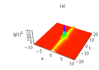
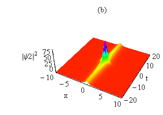
Figure 30: Stabilization of the condensates by finetuning the coupling coefficient for $\nu(t)=0.1t/5$ with the other parameters as in Fig. 28

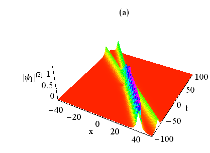
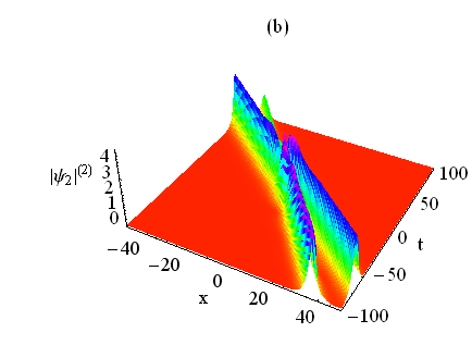
Figure 31: Intramodal Inelastic collision of the condensates without coupling for $a(t)=5,\Gamma(t)=0.1t$ X $10^{-2}$, $\varepsilon_{1}^{(1)}=0.89i$ and $\varepsilon_{1}^{(2)}=0.6$

The profile of the density of the condensates without the linear Rabi coupling is shown in Figs. 27 (a) and (b). When the two condensates are coupled together, one observes an abrupt increase in the density of the condensates as shown in Figs. 28 (a) and (b). This suggests that coupling the two condensates leads to an instability in the dynamical system. However, this instability can be overcome either by changing the temporal scattering length through Feshbach Resonance as shown in Figs. 29 (a) and (b) or by finetuning the time dependent coupling co-efficient as shown in Figs. 30 (a) and (b).

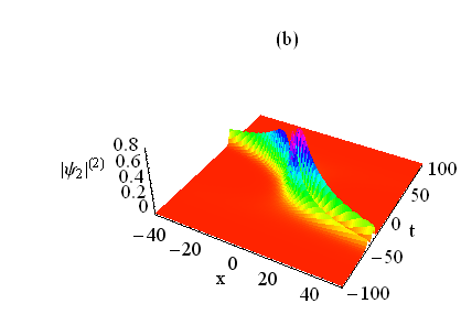
Figure 32: Impact of coupling on the collision of condensates for $\nu(t)=0.01t$ with the other parameters as in Fig. 31

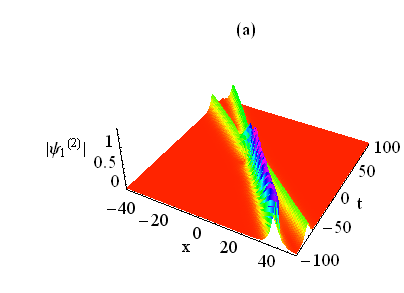
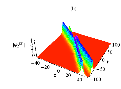
Figure 33: Retrieval of intramodal inelastic interaction of the condensates for $\nu(t)=0.01t$X$10^{-2}$ with the other parameters as in Fig. 32

The gauge transformation approach llc can be easily extended to generate multisoliton solutions. From the collisional dynamics of the condensates, one observes an intramodal inelastic interaction of bright solitons in the absence of weak coupling as shown in Figs. 31(a) and (b). The addition of a weak time dependent coupling disrupts the intramodal inelastic collision of the condensates as shown in Figs. 32(a) and (b). However, one can suitably finetune the coupling coefficient $\nu(t)$ to retrieve the intramodal inelastic collision of the condensates as shown in Figs. 33 (a) and (b).

B. Influence of weak spatially dependent coupling

To understand the effect of weak spatially dependent coupling, we now consider cigar-shaped (quasi-one-dimensional) BECs composed of two hyperfine states of ⁸⁷Rb atoms ref39 confined by the parabolic trapping potential subject to a spatially dependent force $\nu(x)$. The system is now described by the following coupled Gross-Pitaevskii (GP) equation pethick within the framework of the mean-field description as

$$i\psi_{1t}+\psi_{1xx} + 2a(t)(|\psi_{1}|^{2}+|\psi_{2}|^{2})\psi_{1}+\lambda(t)^{2}x^{2}\psi_{1}$$ (127)

$$+ iG(x,t)\psi_{1}+\nu(x)\psi_{2}=0,$$

$$i\psi_{2t}+\psi_{2xx} + 2a(t)(|\psi_{1}|^{2}+|\psi_{2}|^{2})\psi_{2}+\lambda(t)^{2}x^{2}\psi_{2}$$ (128)

$$+ iG(x,t)\psi_{2}+\nu(x)\psi_{1}=0,$$

In the above equations, $\nu(x)$ denotes the weak spatial coupling between the two components while $G(x,t)$ accounts for the feeding which can be carried out by means of a reservoir filled with a large amount of the condensate to which the trap is weakly coupled ref41 . In fact, effects generated by adding the linear coupling to the Manakov model were already studied ref15 and the resulting system was found to be integrable. Equations (127) and (128) have been investigated for $\nu=0$ rajen09 ; twosol.vr.2010 , and the ensuing dynamics of the vectorial BECs has been analyzed. When the trapping potential and (weak) spatial coupling between the two condensates are neglected $(\lambda(t)=\nu(x)=0)$ and the scattering length $a(t)$ becomes a constant (neglecting gain/loss $G(x,t)$) then, the dynamical system becomes the celebrated Manakov’s model ref45 .

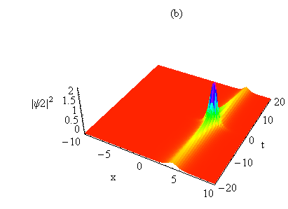
Figure 34: The density of the condensates for $a(t)=0.5t$, $\varepsilon_{1}^{(1)}=0.3$ and $\Gamma(t)=\int 0.005t$ dt in the absence of the coupling.

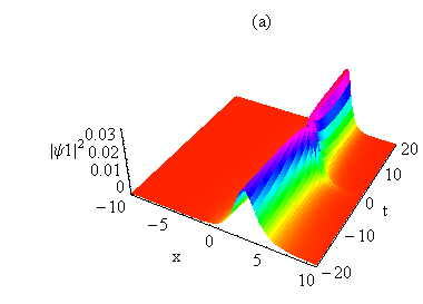
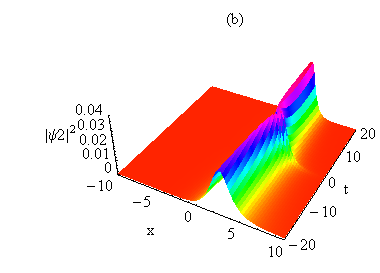
Figure 35: The impact of weak linear coupling $\nu(x)=0.5x$ on the condensates with the other parameters as in Fig. 34

The explicit forms of bright soliton solution of equations (127) and (128) can be written as rrpmypaper

$$\psi_{1}^{(1)}={\frac{2}{\sqrt{a}(t)}}\varepsilon_{1}^{(1)}\beta_{1}(t)\mathrm{sech}(\theta_{1})e^{i(-\xi_{1}+\Gamma(t)\int xdx)},$$ (129)

$$\psi_{2}^{(1)}={\frac{2}{\sqrt{a}(t)}}\varepsilon_{2}^{(1)}\beta_{1}(t)\mathrm{sech}(\theta_{1})e^{i(-\xi_{1}+\Gamma(t)\int xdx)},$$ (130)

where

$$\theta_{1} \equiv 2\int\beta_{1}dx+\int(8\alpha_{1}\beta_{1}-4\alpha_{1})dt-2\delta_{1},$$ (131)

$$\xi_{1} \equiv -2\int\alpha_{1}dx-4\int(\alpha_{1}+4i\beta_{1}^{2}-4\beta_{1})dt-2\chi_{1},$$ (132)

with $\alpha_{1}(t)=\alpha_{10}e^{-2\gamma^{\prime}(t)}$, $\beta_{1}(t)=\beta_{10}e^{-2\gamma^{\prime}(t)}$, where $\delta_{1}$ and $\chi_{1}$ are arbitrary parameters and $\varepsilon_{1,2}$ are coupling parameters.

Thus, it is obvious from equations (129) and (130) that the amplitude of the bright solitons depends on the time-modulated scattering length $a(t)$ and $\beta_{1}{(t)}$, which implicitly depends on $\nu(x)$ (by virtue of equation (7) in Ref. rrpmypaper ). The density profile of the condensates shown in Fig. 34 (a), (b) and Fig. 35 (a), (b) and the time evolution of the bright solitons shown in Fig. 36 demonstrate that, in the absence of spatial coupling, the density of the condensates grows with time while they remain localized around the same point. The introduction of the linear coupling not only stretches the wave packet, but also shifts the center of the localization of the wave packet as shown in Fig. 36.

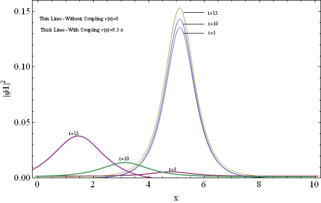
Figure 36: The evolution of bright solitons (given by equation (129)) in the presence and absence of the linear coupling in a confining trap for $\Gamma(t)=\int 0.005t$ dt.

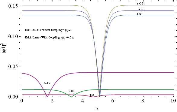
Figure 37: The evolution of a dark soliton (given by equation (133)) in the presence and absence of the spatially-dependent linear coupling in a confining trap for $\Gamma(t)=\int 0.005t$ dt.

The explicit forms of the dark-soliton solution can be written as

$$\psi_{1}^{(1)}=\frac{2}{\sqrt{a(t)}}\varepsilon_{1}^{(1)}\beta_{1}(t)\mathrm{tanh}(\theta_{1})e^{i(-\xi_{1}+\Gamma(x,t)\int xdx)}\\$$ (133)

$$\psi_{2}^{(1)}={\frac{2}{\sqrt{a(t)}}\varepsilon_{2}^{(1)}\beta_{1}(t)\mathrm{tanh}(\theta_{1})e^{i(-\xi_{1}+\Gamma(x,t)\int xdx})}$$ (134)

The time evolution of the dark solitons indicates that one observes a similar impact of the linear coupling (a shift of the center of the localization as shown in Fig. 37 and stretching of the matter wave packet) in the dark solitons as well.

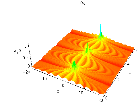
Figure 38: Density profiles of bright-bright soliton interaction for the parametric choice $a(t)=-\cos(\sqrt{2}t),\Gamma(t)=\int 0.001t$ dt, $\nu(x)=\left[\log(-\cos\left(2x\right))\right]^{2}$, $\varepsilon_{1}^{(1)}=0.89i,$ and $\varepsilon_{1}^{(2)}=0.6$ in an expulsive trap.

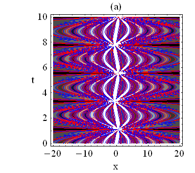
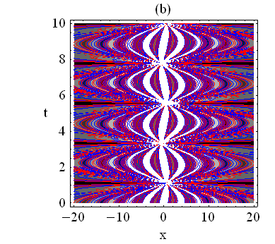
Figure 39: Contour plots for the bright-bright soliton interaction shown in Fig. 38.

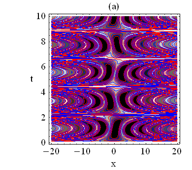
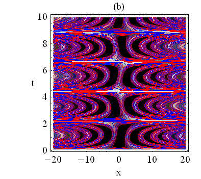
Figure 40: The interference pattern arising from the dark-dark soliton interaction.

Another interesting observation is that the addition of the spatially-dependent linear coupling does not contribute to the growth of the condensates unlike the time-dependent coupling ref37 . Instead, the spatial coupling merely stretches the wave packet. This means that one can easily stabilize the vectorial BECs by the introduction of the spatially-dependent linear coupling. One can easily extend gauge transformation approach to generate multiple dark solitons.

The shift of the center of the matter-wave packet, which is induced by the spatially-dependent coupling, can be suitably exploited to generate matter-wave interference pattern which was addressed theoretically ref51 . The density profile for bright-bright soliton interaction is shown in Figs. 38 (a) and (b). From the density profile, one observes that the matter wave density reaches the maximum value periodically and the central fringe is always bright in every interference pattern. This means that the bright - bright solitons constructively interfere at the centre giving rise to maximum intensity. One observes alternate bright and dark fringes in the pattern. The contour plot shown in Fig. 39 confirms this observation.

The contour plot corresponding to the density profile of dark-dark soliton interaction is shown in Fig. 40. Interference pattern shown in Fig. 40 indicates that the central fringe is always dark indicating that the dark-dark solitons destructively interfere at the centre. Again, one notices alternate dark and bright fringes.

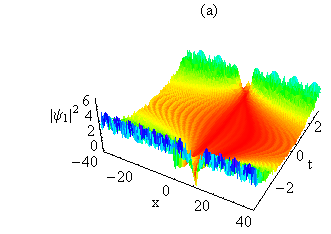
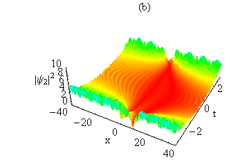
Figure 41: Density profiles for the dark-bright soliton interaction in a transient trap for the parametric choice $\nu(x)=\left[\tan(0.03x)\right]^{2}+0.0075$, $a(t)=0.001t$, $\Gamma(t)=-\int 0.05te^{-0.005t}dt$, $\varepsilon_{1}^{(1)}=0.89i$, and $\varepsilon_{1}^{(2)}=0.6$.

Figure 42: The transient trap for $\Gamma(t)=-\int 0.05te^{-0.005t}dt$.

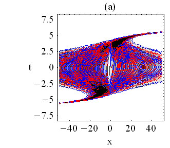
Figure 43: Contour plot of the the dark-bright soliton interaction shown in Fig. 41.

Choosing a transient trap of the form shown in Fig. 42, the density profile of dark-bright interaction is shown in Fig. 41. From the figures, we understand that when the solitons make a transition from the expulsive region to the confining region, the dark and bright solitons interfere with each other in the confining domain. When the trap gets back to the expulsive domain again, the interference pattern disappears while the density of the condensates gets compressed. The above interference pattern is quite identical to the one observed in Ref. rames09pla . From the interference pattern shown in Fig. 43, one observes that the central fringe is always bright indicating the maximum intensity. This occurs because the amplitude of bright solitons predominates over that of the dark solitons. It must be mentioned that the spacing between the bright (or dark) fringes in the interference pattern represented by Figs. 39 and 40 gives a measure of the coherence of matter waves and is a characteristic feature of the atomic system under investigation. The spacing between the bright (or dark) fringes in the interference pattern shown in Fig. 43 observed in the confining trap has narrowed down as the condensates dwell in the confining trap for a very short interval of time.

VII Future Directions

In the present review, we have analytically proved that vector BECs are longlived compared to scalar BECs. Eventhough this paper has comprehensively reviewed the recent developments from the perspective of integrabily in scalar and vector BECs in a time independent/ dependent harmonic trap, there are several unexplored territories in the domain of ultra cold atoms. The identification of an integrable model for a two component BEC (either for a BEC comprising of hyperfine states of the same atom or two different atoms) characterized by three distinct scattering lengths, namely two distinct intraspecies scattering lengths and an interspecies scattering length has eluded our observation so far. Eventhough weak coupling of the condensates generates high density matter waves and one can somehow stabilize them, the question of nonlinearly (strongly) coupling the condensates remains unanswered. These investigations will certainly enable us to penetrate deep into the dynamics of ultra cold atoms with precision. Investigations along these directions are in progress and the results will be published later.

Acknowledgements. RR wishes to acknowledge the financial assistance received from DST (Ref.No:SR/S2/HEP-26/2012 dated 16.10.2012), UGC (Ref.No:F.No 40-420/2011(SR) dated 4.July.2011), DAE-NBHM (Ref.No: NBHM/R.P.16/2014/Fresh dated 22.10.2014) and CSIR (Ref.No: No.03(1323)/14/EMR-II dated 03.11.2014). RR and PSV wish to acknowledge the contribution of Dr. V. Ramesh Kumar in sharing the results of his doctoral thesis. PSV wishes to thank UGC for a Senior Research Fellowship.

References

- (1) W. Crookes Sr., Chemical News 40, 91 (1879).
- (2) M. H. Anderson, J. R. Ensher, M. R. Matthews, C. E. Wieman and E. A. Cornell, Science 269, 198 (1995).
-
(3)
A. Einstein, Sitzber. Kgl. Preuss. Akad. Wiss. 22, 261 (1924);
A. Einstein, Sitzber. Kgl. Preuss. Akad. Wiss. 23, 3 (1925). - (4) S. N. Bose, Z. Phys. 26, 178 (1924).
- (5) E. P. Gross, Nuovo Cimento 20, 454 (1961).
- (6) E. P. Gross, J. Math. Phys. 4, 195 (1963).
- (7) L. P. Pitaevskii, Zh. Eksp. Teor. Fiz. 40, 646 (1961) [Sov. Phys. JETP 13, 451 (1961)].
- (8) S. Inouye, M. R. Andrews, J. Stenger, H. J. Miesner, D. M. Stamper-Kurn, and W. Ketterle, Nature 392, 151 (1998).
-
(9)
J. Weiss, M. Tabor, and G. Carnevale, J. Math. Phys. 24, 522 (1983);
B. Gramaticos and A. Ramani, Integrability of Nonlinear Systems (Springer, Berlin 1997);
M. Lakshmanan and R. Sahadevan, Phys. Rep. 147, 87 (1987);
E. I. Ince, Ordinary differential equations (Dover Publications, New York, 1956);
M. D. Kruskal and P. A. Clarkson, Stud. Appl. Math. 86, 87 (1922). - (10) P. D. Lax, Comm. Pure Applied Math 21, 467 (1968).
- (11) C. S. Gardner, J. M. Greene, M. D. Kruskal, and R. M. Miura, Phys. Rev. Lett. 19, 1095 (1967).
- (12) L.-L. Chau, J. C. Shaw, and H. C. Yen, J. Math. Phys. 32, 1737 (1991).
- (13) G.Darboux, Comptes Rendus Hebdomadaires des Séances de l’Académie des Sciences 94, 1456 (1882)
- (14) V. B. Matveev, Phys. Lett. A 166, 205 (1992).
- (15) V. B. Matveev and M. Salle, Darboux transformations and Solitons (Springer-Verlag, Berlin, 1991).
- (16) R. Hirota and J. Satsuma, Prog. Theor. Phys. Supplement. 59, 64 (1976).
- (17) R. K. Bullough and P. J. Caudrey Solitons (Springer, Berlin, 1980).
- (18) V. E. Zakharov and A. B. Shabat, Soviet Physics JETP 34, 62 (1972).
-
(19)
M.J. Ablowitz, D.J. Kaup, A.C. Newell, and H. Segur, Phys. Rev. Lett. 30, 1262 (1973);
M.J. Ablowitz, D.J. Kaup, A.C. Newell, and H. Segur, Phys. Rev. Lett. 31, 125 (1973). - (20) V. M. Perez-Garcia, H. Michinel, and H. Herrero , Phys. Rev. A 57, 3837 (1998).
- (21) L. Salasnich, A. Parola, and L. Reatto, Phys. Rev. A 65, 043614 (2002).
- (22) Z. X. Liang, Z. D. Zhang, and W. M. Liu, Phys. Rev. Lett. 94, 050402 (2005).
- (23) U. Al Khawaja, J. Phys. A. 39, 9679 (2006).
- (24) R. Radha and V. Ramesh Kumar, Phys. Lett. A, 370, 46 (2007).
- (25) G. Chong and W. Hai, J.Phys. B: At. Mol. Opt. Phys. 40, 211 (2007).
- (26) H.M. Li, Chin. Phys. 15, 2216 (2006).
- (27) E. Kengne and P.K. Talla, J.Phys. B: At. Mol. Opt. Phys. 39, 3679 (2006).
- (28) C. Yuce and A. Kilic, Phys. Scr. 75, 157 (2007).
- (29) L. Wu, J. F. Zhang, and L. Li, New J. Phys. 9, 69 (2007).
- (30) R. Atre, P. K. Panigrahi, and G. S. Agarwal, Phys. Rev. E, 73, 056611 (2006).
- (31) G. Theocharis, Z. Rapti, P. G. Kevrekidis, D. J. Frantzeskakis and V. V. Konotop, Phys. Rev. A. 67, 063610 (2003).
- (32) C. Sulem and P.L. Sulem, The Nonlinear Schrodinger equation, (New York, Springer, 1999).
- (33) L. Khaykovich et al., Science 296, 1290 (2002).
- (34) V. Ramesh Kumar, R. Radha, and P.K. Panigrahi, Phys. Rev. A 77, 023611 (2008).
- (35) J.K. Xue, J. Phys. B: At. Mol. Opt. Phys. 38, 3841 (2005).
- (36) R. Ciuryło, E. Tiesinga, and P. S. Julienne, Phys. Rev. A 71, 030701(R) (2005).
- (37) P. G. Kevrekidis, G. Theocharis, D. J. Frantzeskakis and B. A. Malomed, Phys. Rev. Lett. 90, 230401 (2003).
- (38) D. E. Pelinovsky, P. G. Kevrekidis and D. J. Frantzeskakis, Phys. Rev. Lett. 91, 240201 (2003).
-
(39)
P. Engels, C. Atherton and M. A. Hoefer, Phys. Rev. Lett. 98, 095301 (2007);
A. I. Nicolin, Phys. Rev. E. 84, 056202 (2011). - (40) V. Ramesh Kumar, R. Radha, and P. K. Panigrahi, Phys. Lett. A 373, 4381 (2009).
- (41) M. R. Andrews, C. G. Townsend, H. -J. Miesnor, D. S. Durfee, D. M. Kurn and W. Ketterle, Science 275, 637 (1997).
- (42) J. Javanainen and S. M. Yoo, Phys. Rev. Lett. 76, 161 (1996).
- (43) J. Javanainen, Phys. Rev. Lett. 57, 3164 (1986).
- (44) J. Javanainen, Phys. Lett. A 161, 207 (1991).
- (45) A. Gammal, T. Frederico, L. Tomio, and Ph. Chomaz, J. Phys. B: At. Mol. Opt. Phys. 33, 4053 (2000).
- (46) F. Kh. Abdullaev, A. Gammal, L. Tomio, and T. Frederico, Phys. Rev. A 63, 043604 (2001).
- (47) E. Kengne, R. Vaillancourt, and B. A. Malomed, J. Phys. B: At. Mol. Opt. Phys. 41, 205202 (2008).
- (48) A. Gammal, T. Frederico, and L. Tomio, Phys. Rev. E. 60, 2421 (1999).
- (49) A. Gammal, T. Frederico, L. Tomio, and F. Kh. Abdullaev, Phys. Lett. A 267, 305 (2000).
- (50) T. Khler, Phys. Rev. Lett. 89, 210404 (2002).
-
(51)
J. Denschlag, J. E. Simsarian, D. L. Feder, C. W. Clark, L. A. Collins, J. Cubizolles, L. Deng, E. W. Hagley, K. Helmerson, W. P. Reinhardt, S. L. Rolston, B. I. Schneider, and W. D. Phillips, Science 287, 97 (2000);
S. Burger, K. Bongs, S. Dettmer, W. Ertmer, K. Sengstock, A. Sanpera, G. V. Shlyapnikov, and M. Lewenstein, Phys. Rev. Lett. 83, 5198 (1999). - (52) V. Ramesh Kumar, R. Radha, and M. Wadati, J. Phys. Soc. Jpn. 79, 074005 (2010).
- (53) T. L. Ho and V. B. Shenoy, Phys. Rev. Lett. 77, 3276 (1996).
- (54) B. D. Esry, C. H. Greene, J. P. Burke, and J. L. Bohn, Phys. Rev. Lett. 78, 3594 (1997).
- (55) H. Pu and N. P. Bigelow, Phys. Rev. Lett. 80, 1130 (1998).
- (56) J. Ieda, T. Miyakawa, and M. Wadati, Phys. Rev. Lett. 93, 194102 (2004).
- (57) M. Uchiyama, J. Ieda and M. Wadati, J. Phys. Soc. Jpn. 75, 064002 (2006).
- (58) V. G. Makhankov, N. V. Makhaldiani, and O. K. Pashaev, Phys. Lett. A 81, 161 (1981).
- (59) A. P. Sheppard and Y. S. Kivshar, Phys. Rev. E 55, 4773 (1997).
- (60) M. Wadati, T. Iizuka and M. Hisakado, J. Phys. Soc. Jpn. 61, 2241 (1992).
- (61) Q. H. Park and H. J. Shin, Phys. Rev. E 61, 3093 (2000).
- (62) B. A. Malomed and R. S. Tasgal, Phys. Rev. E 58, 2564 (1998).
- (63) R.Radha, P.S.Vinayagam, and K. Porsezian, Phys. Rev. E. 88, 032903 (2013).
- (64) X-X. Liu, H. Pu, B. Xiong, W. M. Liu, and J.B. Gong, Phys. Rev. A 79, 013423 (2009).
- (65) X. F. Zhang, X-H. Hu, X-X. Liu, W. M. Liu, Phys. Rev. A 79, 033630 (2009).
- (66) S. Rajendran, P. Muruganandam, and M. Lakshmanan, J. Phys. B: At. Mol. Opt. Phys. 42, 145307 (2009).
- (67) V. Ramesh Kumar, R. Radha, and M. Wadati, Phys. Lett. A 374, 3685 (2010).
- (68) R. Radha, P. S. Vinayagam, J. B. Sudharsan, andd Wu-Ming Liu, submitted to J. Phys. B: At. Mol. Opt. Phys. (2014).
- (69) M. R. Matthews, B. P. Anderson, P. C. Haljan, D. S. Hall, M. J. Holland, J. E. Williams, C. E. Wieman, and E. A. Cornell., Phys. Rev. Lett. 83, 3358 (1999).
-
(70)
C. J. Pethick, H. Smith, Bose Einstein Condensation in Dilute Gases (Cambridge Univ. Press, Cambridge, 2003);
L. Pitaeveskii and S. Stringari, Bose Einstein Condensation (Oxford University Press, Oxford, 2003). - (71) M. V. Tratnik and J. E. Sipe, Phys. Rev. A 38, 2011 (1988).
- (72) N. Dror, B. A. Malomed, and J. Zeng, Phys. Rev. E 84, 046602 (2011).
- (73) H. Sakaguchi and B. A. Malomed, Phys. Rev. E 83, 036608 (2011).
- (74) R. Radha and P. S. Vinayagam, Phys. Lett. A 376, 944 (2012).
- (75) M. R. Matthews, B. P. Anderson, P. C. Haljan, D. S. Hall, M. J. Holland, J. E. Williams, C. E. Wieman, and E. A. Cornell, Phys. Rev. Lett. 83, 3358 (1999).
- (76) P. Y. P. Chen and B. A. Malomed, J. Phys. B. 38, 4221 (2005).
- (77) S. V. Manakov, Sov. Phys. JETP 38, 248 (1974).
- (78) R. Radha, P. S. Vinayagam, and K. Porsezian, Rom. Rep. Phys. 66, 427 (2014).
- (79) S. K. Adhikari and B. A. Malomed, Phys. Rev. A 79, 015602 (2009).