Fluctuating Heavy Quark Energy Loss in Strongly-Coupled Quark-Gluon Plasma

Abstract

Results from an energy loss model that includes thermal fluctuations in the energy loss for heavy quarks in a strongly-coupled plasma are shown to be qualitatively consistent with single particle data from both RHIC and LHC. The model used is the first to properly include the fluctuations in heavy quark energy loss as derived in string theory and that do not obey the usual fluctuation-dissipation relations. These fluctuations are crucial for simultaneously describing both RHIC and LHC data; leading order drag results without fluctuations are falsified by current data. Including the fluctuations is non-trivial and relies on the Wong-Zakai theorem to fix the numerical Langevin implementation. The fluctuations lead to surprising results: $B$ meson anisotropy is similar to that for $D$ mesons at LHC, and the double ratio of $D$ to $B$ meson nuclear modification factors approaches unity more rapidly than even predictions from perturbative energy loss models. It is clear that future work in improving heavy quark energy loss calculations in AdS/CFT to include all energy loss channels is needed and warranted.

I Introduction

The goal of heavy ion collision research is to map out the many-body properties of quantum chromodynamics at extreme temperatures. Simultaneously, this research provides insight into the confinement transition of QCD matter and yields information on the earliest moments of the Universe’s existence: currently, no other experimental program can reach back as far in time LRP (2008).

The fireballs created in central RHIC and LHC heavy ion collisions reach temperatures of a trillion degrees Hirano et al. (2011); Shen et al. (2011); Qiu et al. (2012); Gale et al. (2013); at this temperature the many-body dynamics of colored material is very different from that of normal nuclear matter Philipsen (2013). The best way of theoretically understanding this material is not yet known. Simple questions such as “What are the relevant degrees of freedom for the system?” do not yet have a clear answer. At the most basic level, it is not clear how to reconcile experimental results that, naïvely, simultaneously suggest a strongly-coupled plasma that evolves hydrodynamically and a weakly-coupled gas of slightly modified quarks and gluons that yields a plasma relatively transparent to hard probes.

In order to make progress as a field it is necessary to attempt to effect such a reconciliation of ideas of the nature of the plasma into a consistent theoretical picture that yields quantitatively consistent comparisons with experimental data. Focusing on two major avenues of investigations, low transverse momentum (low-$p_{T}$) observables that are described well by near-ideal relativistic hydrodynamics switched on very soon after the initial collision overlap Hirano et al. (2011); Shen et al. (2011); Qiu et al. (2012); Gale et al. (2013) and high-$p_{T}$ observables associated with hard production described by perturbative quantum chromodynamics (pQCD) Majumder and Van Leeuwen (2011); Horowitz (2013); Djordjevic et al. (2014), the low-$p_{T}$ observables appear readily understood within a strong-coupling paradigm for the plasma in which calculations are performed using the AdS/CFT correspondence Gubser et al. (1996); Kovtun et al. (2005); Casalderrey-Solana et al. (2011) while the high-$p_{T}$ observables appear readily understood within a weak-coupling paradigm for the plasma in which calculations are performed using pQCD Majumder and Van Leeuwen (2011).

Specifically, leading order derivations exploiting the AdS/CFT correspondence found that quark-gluon plasma (QGP)-like systems have thermodynamic properties such as entropy density similar to those seen from the lattice Gubser et al. (1996); Philipsen (2013); rapidly hydrodynamize after a heavy ion collision-like event Chesler and Yaffe (2011), i.e. nearly ideal relativistic hydrodynamics approximates well the dynamics of the system soon after a heavy ion collision as is inferred from data; and have a very small shear viscosity-to-entropy ratio $\eta/s\,\sim\,0.1$ in natural units Gubser et al. (1996); Kovtun et al. (2005), again as inferred from hydrodynamics studies of data Hirano et al. (2011); Shen et al. (2011); Qiu et al. (2012); Gale et al. (2013). At the same time, leading order derivations based on pQCD show differences to thermodynamic properties Cheng et al. (2008), do not hydrodynamize rapidly Attems et al. (2013), and have a viscosity-to-entropy ratio $\eta/s\,\sim\,1$ Danielewicz and Gyulassy (1985) at least an order of magnitude larger than that inferred from hydrodynamics.

On the other hand, energy loss models for light and heavy flavored particles based on calculations using leading order pQCD show broad qualitative agreement with data from both RHIC and LHC Majumder and Van Leeuwen (2011); Horowitz (2013); Djordjevic et al. (2014). At the same time, early light flavor Horowitz and Gyulassy (2011) and leading order heavy flavor Horowitz (2012) energy loss models using AdS/CFT found or suggested a massive oversuppression of high-$p_{T}$ leading particles compared to data.

Much work has been done to improve perturbative field theoretic treatments of soft, or low-$p_{T}$, observables. For example there are high-order thermal field theory calculations of thermodynamic properties of the QGP Haque et al. (2014) and recent work suggested that pQCD can yield rapid isotropization times of $0.2-1.0$ fm Kurkela and Lu (2014). The small viscosity-to-entropy ratio inferred from hydrodynamics remains a challenge for perturbative calculations; no pQCD calculation has yet yielded $\eta/s\,\sim\,0.1$.

An alternative research avenue is to improve the AdS/CFT treatment of high-$p_{T}$ observables. There are hybrid calculations in which, for instance, AdS/CFT is used to model the medium only Gubser (2008); Casalderrey-Solana and Teaney (2007); D’Eramo et al. (2011) or only part of the energy loss Casalderrey-Solana et al. (2014), although in the latter case the coupling is taken to be quite small, $\lambda\,\sim\,10^{-3}-10^{-4}$. Other work has attempted to apply AdS/CFT to the entire energy loss problem. A recent success Morad and Horowitz (2014) found that when the strong-coupling jet prescription is improved and the in-medium energy loss is renormalized, a reasonable value of $\lambda\,=\,5.5$ yielded a jet nuclear modification factor $R_{AA}^{jet}(p_{T})$ quantitatively consistent with preliminary CMS data Collaboration (2012).

By allowing the variation of the intrinsic mass of the probe, heavy quark observables provide an extremely valuable additional test of energy loss calculations and, therefore, the properties of quark-gluon plasma. It has been very fruitful for the energy loss community to require of energy loss models a simultaneous description of both light and heavy flavor observables. For example, Djordjevic et al. (2006) showed that pQCD-based energy loss models that only include the radiative energy loss channel could not simultaneously describe both suppression of particles associated with both light and heavy flavors at RHIC. From the strong-coupling side of calculations, heavy quark observables are especially useful as the theory of heavy quark energy loss is both more mature and under better control than that for light flavors Gubser (2006); Herzog et al. (2006); Casalderrey-Solana and Teaney (2006); Chesler et al. (2009); Ficnar (2012); Morad and Horowitz (2014).

The work of this paper is to improve the energy loss modelling of heavy quarks under the assumption of a strongly-coupled medium strongly-coupled to the heavy quark. Previous calculations that used only the leading order strongly-coupled heavy quark energy loss, often referred to as heavy quark drag, compared favorably to the measured nuclear modification factor $R_{AA}(p_{T})$ of electrons from heavy flavor decay at RHIC Horowitz (2010) but generally oversuppressed $R_{AA}(p_{T})$ for $D$ mesons at LHC by a factor of $\sim\,5$ Horowitz (2012). Another early comparison to RHIC data included fluctuations in the energy loss as dictated by the fluctuation-dissipation theorem Akamatsu et al. (2009). These results were consistent with data from RHIC, but were never compared to data from LHC. A major deficiency of the approach of Akamatsu et al. (2009) is that the string theoretic derivation of the thermal momentum fluctuations for heavy quarks Gubser (2008) demonstrated that the momentum diffusion is not related to the momentum drag according to the fluctuation-dissipation theorem. Even worse, the fluctuations are non-Markovian; the fluctuations are due to colored noise, which means that there are non-trivial temporal correlations between the momentum kicks.

In this paper the correct fluctuation spectrum is used and the non-Markovian nature of the momentum fluctuations is mitigated; it will be shown that by doing so one can qualitatively describe the data related to single heavy flavor observables at both RHIC and LHC simultaneously.

II Langevin Energy Loss

It was shown in Gubser (2008) that the three-momentum $p^{i}$ of an on-shell heavy quark moving at constant velocity in a thermal bath evolves as:

$$\frac{dp_{i}}{dt}=-\mu\,p_{i}+F_{i}^{L}+F_{i}^{T},$$ (1)

where the drag coefficient Gubser (2006); Herzog et al. (2006); Casalderrey-Solana and Teaney (2006) of a heavy quark of mass $M_{Q}$ in a plasma of temperature $T$ with ’t Hooft coupling $\lambda$ is

$$\mu=\frac{\pi\sqrt{\lambda}T^{2}}{2M_{Q}}$$ (2)

and the fluctuating momentum kicks are correlated as

$$\langle F_{i}^{L}(t_{1})F_{j}^{L}(t_{1})\rangle =\kappa_{L}\hat{p}_{i}\hat{p}_{j}g(t_{2}-t_{1})$$ (3)

$$\langle F_{i}^{T}(t_{1})F_{j}^{T}(t_{1})\rangle =\kappa_{T}(\delta_{ij}-\hat{p}_{i}\hat{p}_{j})g(t_{2}-t_{1}),$$ (4)

where $\hat{p}_{i}\,=\,p_{i}/|\vec{p}|$,

$$\kappa_{T} =\pi\sqrt{\lambda}T^{3}\gamma^{1/2}$$ (5)

$$\kappa_{L} =\gamma^{2}\kappa_{T},$$ (6)

and $g$ is a function known only numerically.

Since the fluctuations increase in magnitude with heavy quark velocity—in fact increase very, very quickly in the longitudinal direction (like $\gamma^{5/2}$), which is the most important direction for calculations of suppression observables—one may naturally ask: at what speed should one expect the fluctuations to play a nontrivial role in heavy quark energy loss? This speed limit may be estimated by requiring that the momentum picked up via fluctuations over the time scale set by the drag coefficient be small in comparison to the total momentum of the heavy quark. One finds then an upper limit on the speed of the heavy quark given by

$$\gamma\lesssim\gamma_{crit}^{fluc}=\frac{M_{Q}^{2}}{4T^{2}}.$$ (7)

There is a well-known speed limit for the heavy quark drag setup in which the derivation of Eq. (1) was performed. A finite mass heavy quark is represented by a string connected to a D7 brane that partially fills the fifth dimension Karch and Katz (2002). The mass of the heavy quark is related to the depth that the D7 brane fills the fifth dimension; the greater the depth, the lighter the quark. In a space with a black hole—dual to a plasma at finite temperature Witten (1998)—the local speed of light decreases with the depth of the fifth dimension. Thus in this setup the endpoint of a string dual to a finite mass heavy quark that is connected to the bottom of the D7 brane has as a natural speed limit the local speed of light Gubser (2008); a heavy quark in the field may move faster than this speed, but then the setup is necessarily incorrect for this physical situation. Equivalently, the speed limit can be derived from self-consistency: in the setup in which the drag formulae are derived, the heavy quark moves at a constant velocity. In order for the constant velocity to be maintained, one must provide power to the heavy quark to balance the momentum lost. If that power is provided by a gauge field, there is a maximum field strength before which Schwinger pair production begins; that maximum field strength limits the velocity with which the quark can be pulled through the plasma at a constant velocity Casalderrey-Solana and Teaney (2007). Both lines of reasoning lead to exactly the same speed limit. This speed limit on the heavy quark setup leads to the requirement that

$$\gamma<\gamma_{crit}^{sl}=\big{(}1+\frac{2M_{Q}}{\sqrt{\lambda}T}\big{)}^{2}\sim\frac{4M_{Q}^{2}}{\lambda T^{2}}.$$ (8)

One may easily see that parametrically the critical speed is restricted most by the speed limit due to the requirement of constant heavy quark velocity, not due to the momentum kicks picked up from the medium; the former goes as $\lambda^{-1}$ while the latter goes as $\lambda^{0}$. However, in the case of finite $\lambda\sim\mathcal{O}(10)$ one finds that the critical speed due to momentum fluctuations is actually smaller than that of the speed limit. It is therefore important to include these fluctuations in a phenomenological heavy quark energy loss model based on AdS/CFT that is compared to data, the goal of this work.

The implementation of the fluctuations in Eq. (1) are nontrivial for two reasons: first, the noise is colored and second, the fluctuations are multiplicative. With respect to the former complication, if $g$ was a Dirac delta function, the momentum fluctuations in Eq. (1) would correspond to white noise; i.e. one momentum kick is not correlated in time with any other. However, it was shown in Gubser (2008) that the noise is actually colored, in which case $g$ is some nontrivial function of characteristic width $t_{corr}\sim\sqrt{\gamma}/T$. With respect to the latter complication, multiplicative noise has correlations that depend on the dynamical variable, in this case $p_{i}$. Unlike usual Riemann calculus, stochastic Ito integration is sensitive to the precise location at which the integrand is evaluated within a time step; different choices of location within the time step yield different results for the integral Evans (2013); Gardiner (2009); van Kampen (2007); Kloeden and Platen (1995). Note that these different results for the integral are truly fundamental and not due to finite size time steps. Unfortunately, the work of Gubser (2008) did not specify at which place within the time step the derived fluctuations should be applied. Fig. 1 shows the significant differences in the momentum distributions of charm quarks in a thermal plasma of $T\,=\,400$ MeV which is moving at $v\,=\,0.9\,$c in the $z$ direction for three different but common choices made for the location within the time step to apply the momentum fluctuation. In particular the results for the Itô (pre-point, for which the integrand and the fluctuation are evaluated at the earliest time within a time step), Stratonovich (mid-point, for which the integrand and the fluctuation are evaluated at the middle of a time step), and Hänggi-Klimontovich (post-point, for which the integrand and the fluctuation are evaluated at the latest time within a time step) rules are shown. The differences between rules are especially pronounced in the tails of the distribution (c.f. Fig. 1 (LABEL:sub@subfig:dNdpz)), which tends to be the most important for the purposes of energy loss modeling. Note that none of the distributions produced by the different integration prescriptions for the momentum fluctuations given by AdS/CFT are exactly thermal. The deviation away from the thermal distribution can be attributed at least in part to the modification of the usual dispersion relation of the heavy quark due to its coupling to the strongly-coupled thermal medium Herzog et al. (2006). In Fig. 1 the relativistic Maxwell-Boltzmann, or Jüttner, distribution is shown and compared to a distribution produced by a Langevin evaluation whose diffusion coefficient is related to its drag via the relativistic fluctuation-dissipation relation He et al. (2013). This comparison between the analytic and numerical results is a non-trivial cross check of both the analytics and numerics: the distribution along the direction of plasma fluid flow, Fig. 1 (LABEL:sub@subfig:dNdpz), is not a trivial boost of the distribution along a direction for which the plasma is at rest, Fig. 1 (LABEL:sub@subfig:dNdpz); see Appendix A.

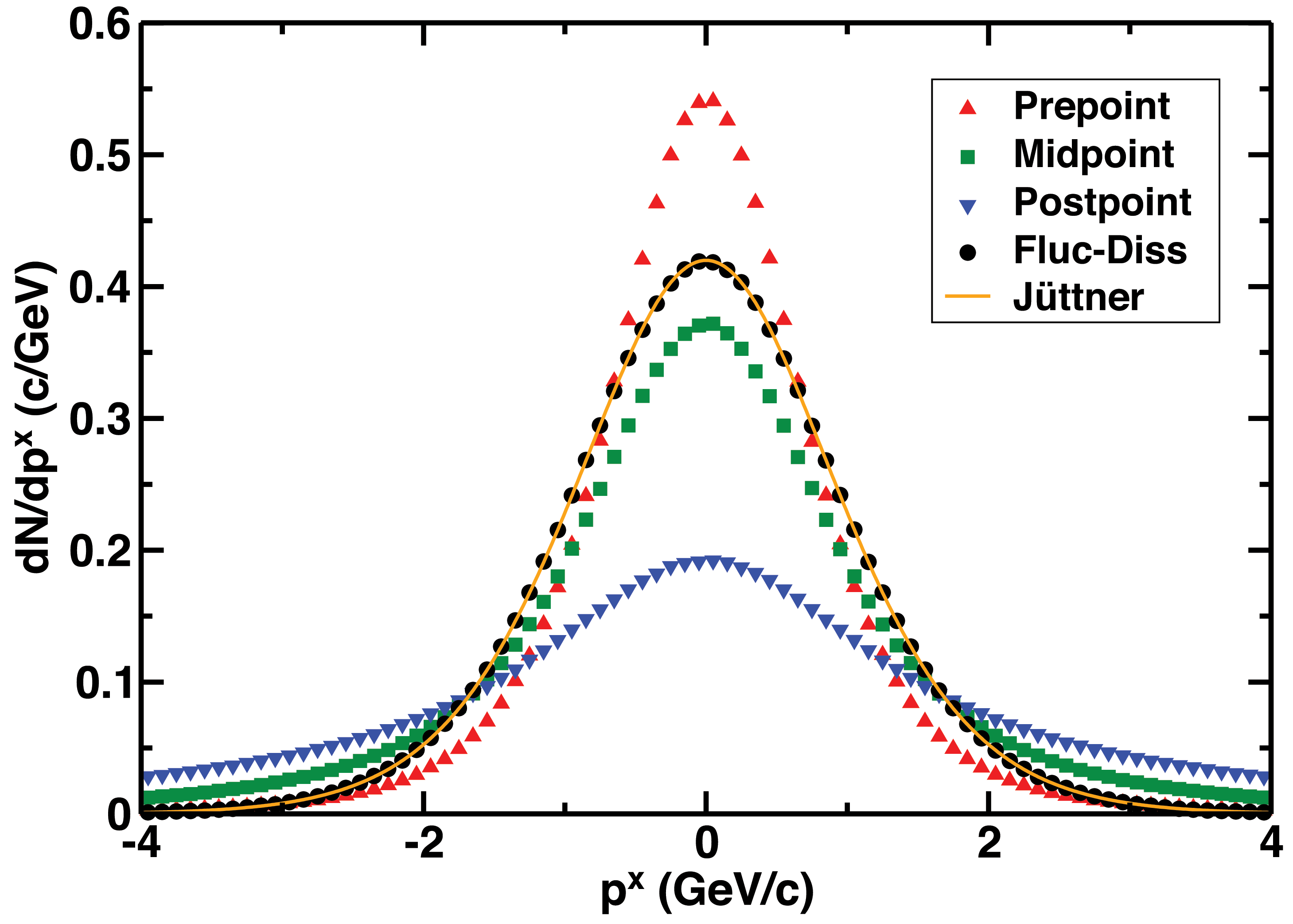
(a)

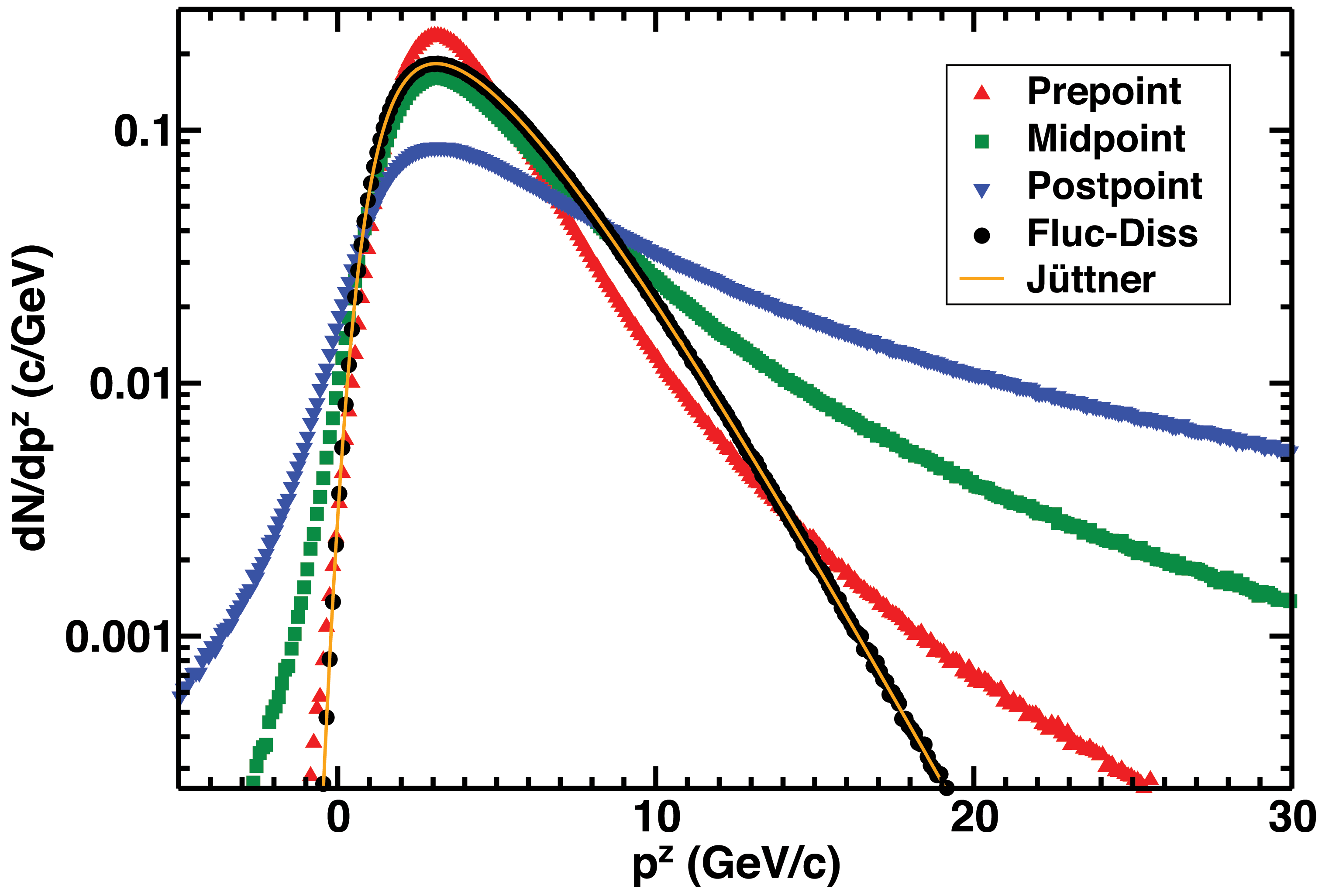
(b)

Figure 1: (LABEL:sub@subfig:dNdpx) The $p^{x}$-differential distribution of $m_{c}\,=\,1.5$ GeV$/$c² charm quarks strongly-coupled to a strongly-coupled plasma in three spatial dimensions at $T\,=\,400$ MeV which is moving at $0.9\,$c in the $z$ direction. The effect of the thermal drag and fluctuations on the heavy quarks from strong coupling is found from implementing Eq. (1) using the Itô (pre-point), Stratonovich (mid-point), and Hänggi-Klimontovich (post-point) stochastic integrals. An implementation for which the fluctuation-dissipation theorem holds is also shown and compared to the result expected, the Jüttner distribution. (LABEL:sub@subfig:dNdpz) The same as (LABEL:sub@subfig:dNdpx) but for the $p^{z}$-differential distribution.

Fortunately, both the colored and multiplicative complications of the noise can be handled. As for the first complication, in every physical situation, all noise is actually colored (for example the air molecule that just collided with a floating pollen grain cannot immediately collide with the pollen grain again); the issue is whether or not the time scale over which the momentum kicks are correlated is small compared to the other relevant time scale(s) in the problem. For heavy quark energy loss as computed at strong coupling in AdS/CFT, the only other relevant time scale is determined by the drag coefficient $\mu$ from Eq. (1). One may check that

$$t_{corr}\mu\sim\frac{1}{2}\sqrt{\lambda}\sqrt{\gamma}\frac{T}{M_{Q}}<1$$ (9)

so long as $\gamma\,<\,\gamma_{crit}^{sl}$ from Eq. (8). Thus we are able to approximate the colored noise as white noise so long as the heavy quark is moving slower than the speed limit imposed by the setup of the derivation. As for the second complication, there is a theorem due to Wong and Zakai Wong and Zakai (1965) that proves that in the limit that the autocorrelation time for noise goes to zero, the correct stochastic integral is the Stratonovich one, which is to say that the integrand and noise terms are evaluated at the midpoint of the time step. As just noted, for the specific calculation of interest in this work, the autocorrelation time is small so long as the heavy quark moves more slowly than the speed limit $\gamma_{crit}$, Eq. (8).

In the energy loss model used in this paper, the stochastic differential equation Eq. (1) was solved numerically using the Euler-Maruyama scheme Kloeden and Platen (1995). Despite its simplicity, the Euler-Maruyama scheme converges strongly, and the scheme was sufficient for the purposes in this paper. (Higher order strongly convergent schemes exist, e.g. Milstein, but are highly non-trivial to implement for motion in more than one dimension.) In any implementation of a stochastic integral, whether Itô, Hänggi-Klimontovich, or anything in-between, one may actually evaluate the integral in any other choice with the addition (or subtraction) of the appropriate terms Kloeden and Platen (1995); Gardiner (2009). In particular an Itô (pre-point) stochastic differential equation

$$dp^{i}=a^{i}\big{(}t,\,p^{k}(t)\big{)}dt+b^{ij}\big{(}t,\,p^{k}(t)\big{)}dW_{j}$$ (10)

with Wiener process $dW^{j}$ is equivalent to the Stratonovich stochastic differential equation of the form

$$dp^{i}=\underline{a}^{i}\big{(}t,\,p^{k}(t)\big{)}dt+b^{ij}\big{(}t,\,p^{k}(t)\big{)}\circ dW_{j},$$ (11)

where

$$a^{i}\big{(}t,\,p^{k}(t)\big{)}=\underline{a}^{i}\big{(}t,\,p^{k}(t)\big{)}\\ +\frac{1}{2}\sum_{\ell}\sum_{m}b^{\ell m}\big{(}t,\,p^{k}(t)\big{)}\frac{\partial b^{im}}{\partial p^{\ell}}\big{(}t,\,p^{k}(t)\big{)}.$$ (12)

For ease of numerics, all results shown in this work had the integrand and noise terms evaluated at the earliest moment in the time step (Itô, or, pre-point). Thus in the local fluid rest frame the momentum components of a heavy quark at the next time step, $p^{\prime i}_{n+1}$, were found from the momenta at the current time step, $p^{\prime i}_{n}$, by interpreting Eq. (1) as a Stratonovich stochastic differential equation, modified by Eq. (12) to be implemented as an Itô SDE in the Euler-Maruyama scheme with the result that

$$p^{\prime i}_{n+1}=\Big{(}1-\mu\,dt^{\prime}+\frac{1}{2}\kappa\,dt^{\prime}\big{(}\,\frac{5\gamma^{5/2}}{4E^{\prime 2}}\\ +\frac{(d-1)\,\gamma^{1/2}}{(\gamma^{2}+1)\,m^{2}}\,\big{)}\Big{)}p^{\prime i}_{n}+C^{ij}dW_{j},$$ (13)

where $\mu$ is given by Eq. (2); $dt^{\prime}$ is the time step $dt$ boosted into the local rest frame of the fluid; $dt^{\prime}\,=\,dt/\gamma$; $\kappa\,=\,\pi\sqrt{\lambda}T^{3}$, where $T$ is the temperature of the fluid in its local rest frame; $d$ is the number of spatial dimensions in the calculation (in this case we propagate the heavy quarks through backgrounds generated by VISHNU Shen et al. (2011); Qiu et al. (2012), which is a $2+1D$ hydrodynamics code); the $dW_{j}$ are the uncorrelated, Gaussian Wiener kicks with mean 0 and standard deviation 1; and

$$C^{ij} =\sqrt{dt^{\prime}\,\kappa}\gamma^{1/4}\left(\frac{p^{\prime i}p^{\prime j}}{(\gamma^{2}+1)\,m^{2}}+\delta^{ij}\right).$$ (14)

In a calculation that follows the trajectory of the heavy quark from production onwards, at each time step the code boosts into the local rest frame of the fluid, evaluates the change in momentum, boosts back to the lab frame, and propagates the heavy quark in coordinate space according to

$$x^{i}_{n+1}=\frac{p^{i}_{n+1}}{E_{n+1}}dt.$$ (15)

$dt$ was taken to be $1/150\times\mu_{max}$, where $\mu_{max}$ is the drag coefficient at the center of the fireball at the thermalization time, the largest drag coefficient for any individual collision. This value of $dt$ was found through trial and error to consistently yield stable static thermal distributions such as those shown in Fig. 1. Variations of $dt$ by a factor of 2 in both directions yielded unchanged results in trials. The code was written in C++, compiled using Clang, and run on a Mac laptop.

III Energy Loss Model

The results presented here are from a fully Monte-Carlo energy loss model; only the fragmentation from heavy quarks into their decay products was handled through (numerical) integration of analytic expressions. In particular, the production spectrum for heavy quarks (from FONLL Cacciari et al. (1998, 2001, 2012)), the spatial distribution of their production points (weighed by the Glauber binary distribution Miller et al. (2007)), and their initial direction of propagation (assumed uniform) were randomly sampled. Propagation was through backgrounds generated by the VISHNU 2+1D hydrodynamics code Shen et al. (2011); Qiu et al. (2012), with momenta updated according to Eq. (1). (Pseudo-) random number generation was performed using the Ran routine from Numerical Recipes Press et al. (2007). Seed generation came from the routine described in Katzgraber , which is appropriate for running multiple processes at or nearly at identical times on multiple processors.

The production spectrum and fragmentation functions of the heavy quarks from FONLL were used Cacciari et al. (1998, 2001, 2012). The spectra were generated by the FONLL web page FON for the relevant center of mass and rapidity ranges for the various experiments. The fragmentation functions from heavy quarks to heavy mesons were taken from Cacciari et al. (2012). For measurements of unspecified $D$ mesons (and for electrons from $D$ mesons), the FONLL approximation of $D$ mesons being comprised of 70% $D^{0}$ and 30% $D^{+}$ mesons was used FON . The semi-leptonic decay of heavy mesons to electrons is not given explicitly in any FONLL paper. The probability $P(E)$ of a heavy meson decaying to an electron of energy $E$ in the rest frame of the heavy meson used in Cacciari et al. (2005) was provided Vogt and Cacciari , but detailed instructions for implementation were not. One may calculate the distribution of electrons in the lab frame from the semi-leptonic decay of a heavy meson; the details are given in Appendix B. In particular, Eqs. (26) and (B) – (B) are used throughout the rest of this work for the fragmentation of heavy mesons to electrons and $B$ mesons to $J/\psi$ mesons.

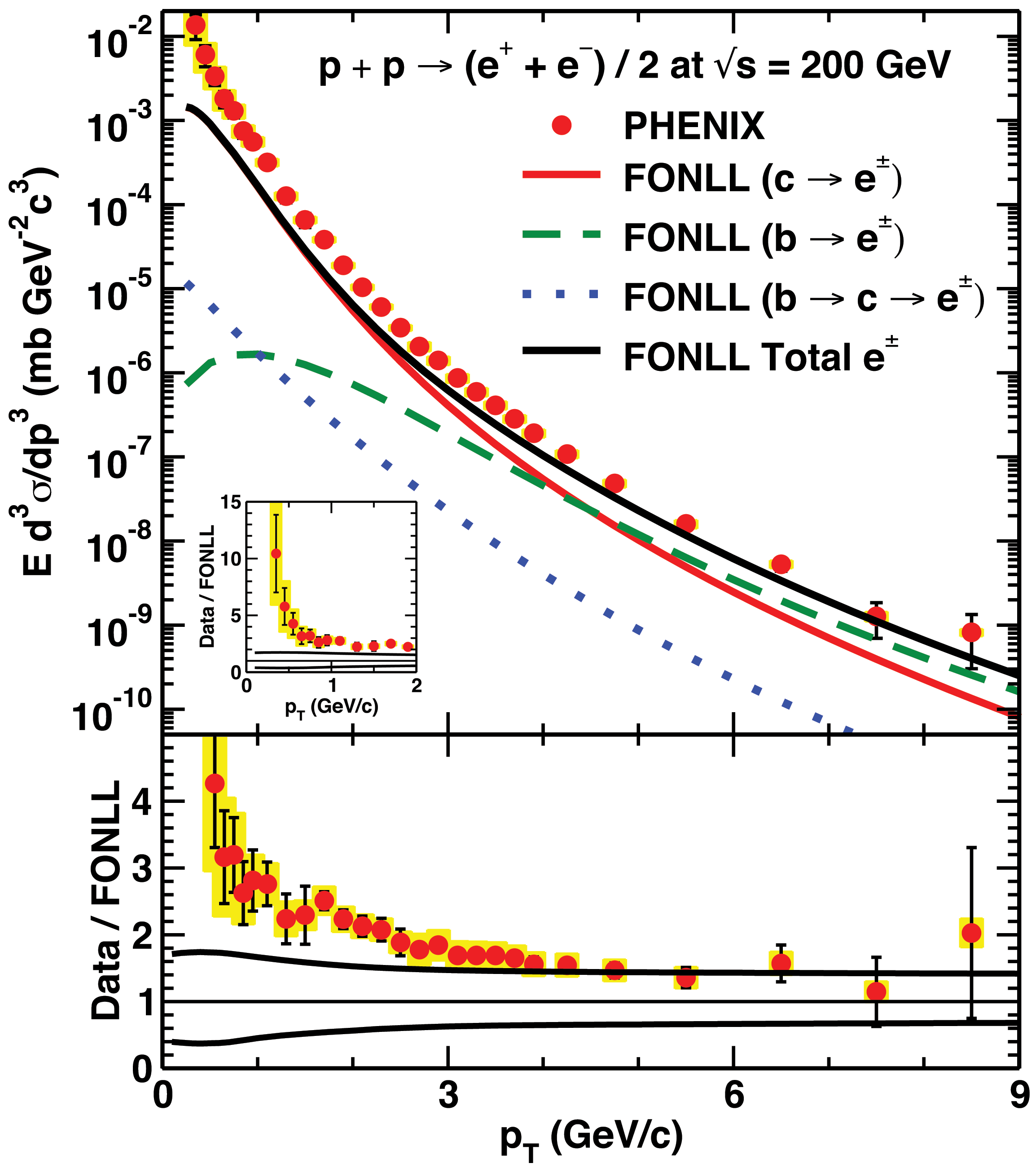
Figure 2: (Top) A comparison of FONLL predictions Cacciari et al. (1998, 2001, 2012) for the electron spectrum from open heavy flavor production in $p+p$ collisions at $\sqrt{s}\,=\,200$ GeV to that measured by PHENIX Adare et al. (2011). (Bottom) Ratio of the PHENIX data to FONLL predictions; the solid black lines represent the uncertainty in the FONLL predictions due to scale variations. (Inset) Zoom in on the low-$p_{T}$ part of the ratio of data to FONLL predictions showing the full range of disagreement.

The production spectrum of electrons originating from open heavy flavor in $p+p$ collisions at $\sqrt{s}\,=\,200$ GeV from FONLL is compared to that measured by PHENIX Adare et al. (2011) at RHIC in Fig. 2. One can see that at ultrarelativistic momenta, the FONLL predictions are consistent with the data within the experimental and theoretical uncertainties, which amount to approximately a factor of 2. At lower momenta the FONLL predictions deviate more, rising to a discrepancy of an order of magnitude for the smallest measured momentum bin of $p_{T}\,=\,0.25$ GeV/c. For electrons it appears that the production and/or the fragmentation description is not reliable below $p_{T}^{e}\,\lesssim\,3$ GeV/c. (It seems likely that the issue is with the fragmentation to electrons, with the discrepancy made much worse by the experimentally restricted rapidity range.)

When computing the energy loss and fluctuations, one needs a mapping from the QCD parameters to the $\mathcal{N}\,=\,4$ SYM parameters. Results in this paper are shown using two prescriptions, which are denoted in the plots “$\alpha_{s}\,=\,0.3$” and “$\lambda\,=\,5.5$,” in order to explore a reasonable breadth of possibilities (one hopes that a calculation in a theory dual to QCD would lie somewhere between these two prescriptions). For the former, the ’t Hooft coupling is taken to be $\lambda\,=\,4\pi\alpha_{s}N_{c}\,=\,4\pi\times 0.3\times 3$ and $T_{QCD}\,=\,T_{SYM}$. For the latter, the prescription of Gubser (2008) is followed, in which $\lambda\,=\,5.5$ and $T_{SYM}\,=\,T_{QCD}/3^{1/4}$. The masses of the quarks were taken to be $m_{c}\,=\,1.5$ GeV$/$c² and $m_{b}\,=\,4.75$ GeV$/$c².

IV Results

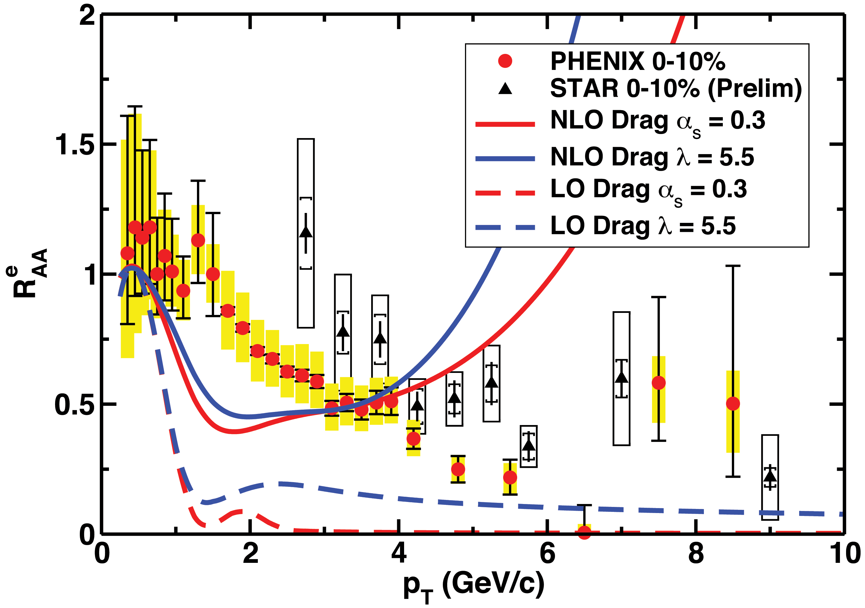
(a)

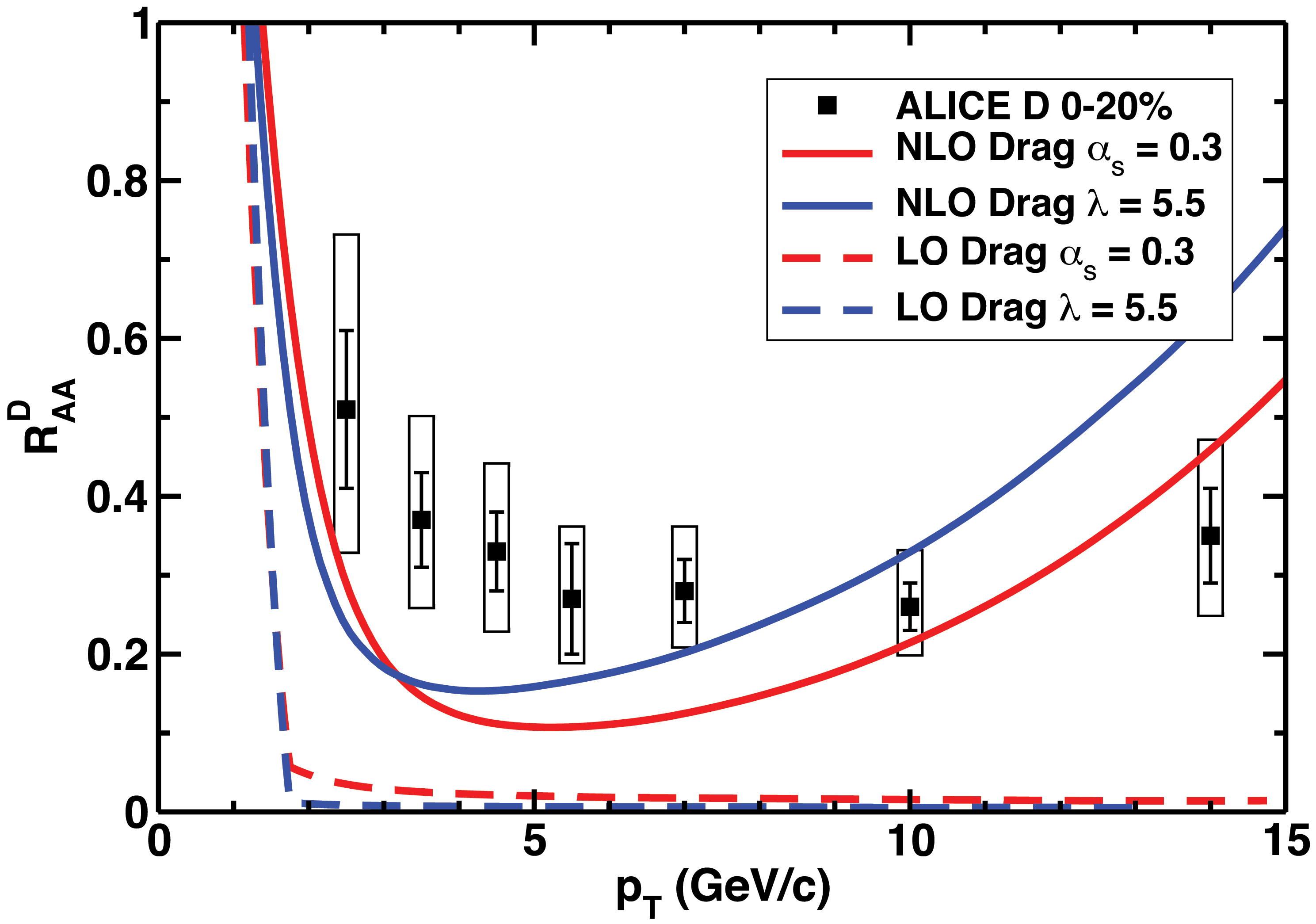
(b)

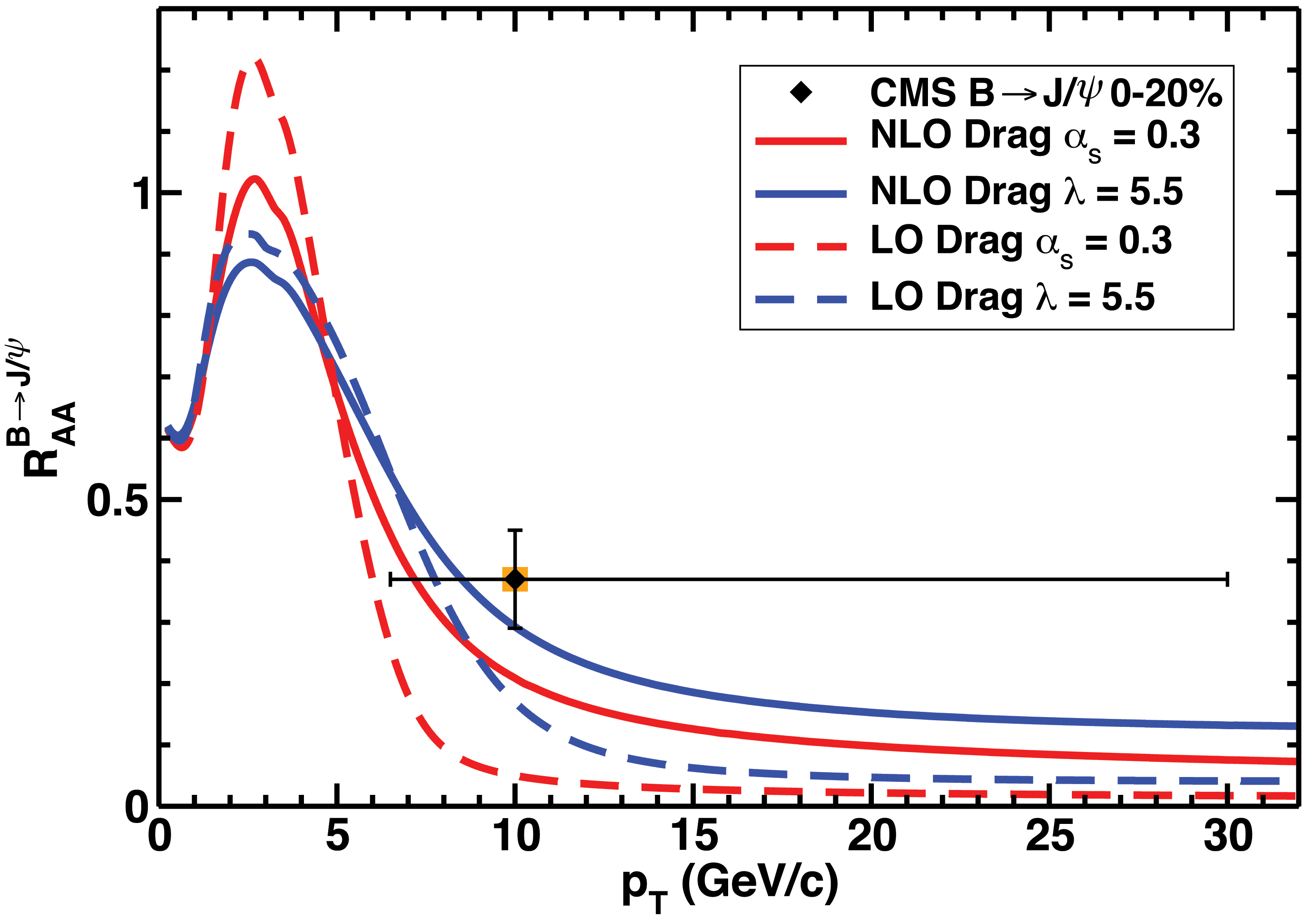
(c)

Figure 3: (LABEL:sub@subfig:RHICe) Open heavy flavor electron $R_{AA}(p_{T})$ at RHIC measured by PHENIX Adare et al. (2011) and STAR Mustafa (2013) compared to predictions from heavy quark drag only (“LO”) and heavy quark drag with fluctuations (“NLO”) energy loss models. (LABEL:sub@subfig:LHCD) $D$ meson $R_{AA}(p_{T})$ at LHC measured by ALICE Abelev et al. (2012) compared to the strongly-coupled energy loss predictions. (LABEL:sub@subfig:LHCBJpsi) Non-prompt $J/\psi$ meson $R_{AA}(p_{T})$ at LHC measured by CMS Chatrchyan et al. (2012) compared to the energy loss model predictions. For curves labeled $\alpha_{s}\,=\,0.3$, $\lambda\,=\,4\pi\times 0.3\times 3$ and $T_{SYM}\,=\,T_{QCD}$; for curves labeled $\lambda\,=\,5.5$, $T_{SYM}\,=\,T_{QCD}/3^{1/4}$.

Fig. 3 shows the main results of this paper: predictions for $R_{AA}(p_{T})$ for electrons from open heavy flavor at RHIC, $D$ meson suppression at LHC, and non-prompt $J/\psi$ suppression at LHC all compared to data Adare et al. (2011); Mustafa (2013); Abelev et al. (2012); Chatrchyan et al. (2012). When including only the leading order drag without fluctuations, the model significantly oversuppresses the nuclear modification factor compared to data. But when the correct fluctuations are included, the predictions—within their regime of applicability—are in qualitative agreement with all current suppression data.

To expand on the point of the regime of applicability, while the electron prediction below $p_{T}\,\lesssim\,3$ GeV/c is not in particularly good agreement with data, the electron production and/or fragmentation functions are untrustworthy below this momentum scale. The regime of applicability is also crucial to note as it explains the dramatic increase in $R_{AA}$ for electrons and $D$ mesons for momenta beyond a few GeV/c ($\gtrsim\,4$ GeV/c for electrons and $\gtrsim\,10$ GeV/c for $D$ mesons): self-consistently, one sees that at momenta of order the speed limit, the momentum fluctuations begin to dominate at the momenta at which the setup of the problem is breaking down. The lack of inclusion of Larmor-like energy loss Mikhailov (2003); Fadafan et al. (2009) due to what would be significant deceleration becomes a poor approximation, as is the white noise assumption for the fluctuations. When that important physics is included, the rapid rise in $R_{AA}(p_{T})$ above $p_{T}\,\gtrsim\,4-5$ GeV/c will be tamed, although the magnitude of the effect is not yet known or estimable.

In previous work Horowitz (2010), drag-only strong-coupling energy loss gave a good quantitative description of RHIC electron data, but, when using the same parameters, predicted an oversuppression of $D$ mesons at LHC Horowitz (2012), due to the very sensitive $\mu\,\sim\,T^{2}$ nature of the drag. In this calculation there is already an oversuppression at RHIC. It is precisely this considerable sensitivity to temperature that leads to an oversuppression at RHIC in this calculation: the VISHNU hydrodynamics Shen et al. (2011); Qiu et al. (2012) is significantly hotter than the Glauber model used in the previous work Horowitz (2010).

One may also compare to other observables, for instance the azimuthal anisotropy of the $D$ mesons, as shown in Fig. 4. The energy loss model including fluctuations qualitatively agrees with the experimental results from ALICE Abelev et al. (2013), although with a generic underprediction for the $v_{2}$ at intermediate-$p_{T}$ values $p_{T}\,\lesssim\,10$ GeV/c. This underprediction in $D$ mesons is reminiscent of the underprediction of $v_{2}$ for light flavor observables in pQCD-based energy loss models Shuryak (2002); Horowitz (2006) and, like in the light flavor case, probably indicates a modification of the fragmentation process that enhances the anisotropy in this momentum range. Future measurements with increased statistics will, as in the light flavor case Aad et al. (2012); Horowitz and Gyulassy (2011), presumably show that the $D$ meson $v_{2}$ decreases as a function of $p_{T}$ to levels similar to the energy loss predictions. Predictions for $B$ meson $v_{2}$ from the energy loss model are also shown in Fig. 4; surprisingly, the model predicts $B$ meson $v_{2}$ of a similar size as the $D$ meson $v_{2}$. It will be very interesting to see if measurements of the $B$ meson $v_{2}$ are of a similar magnitude to the $D$ meson $v_{2}$ as predicted here.

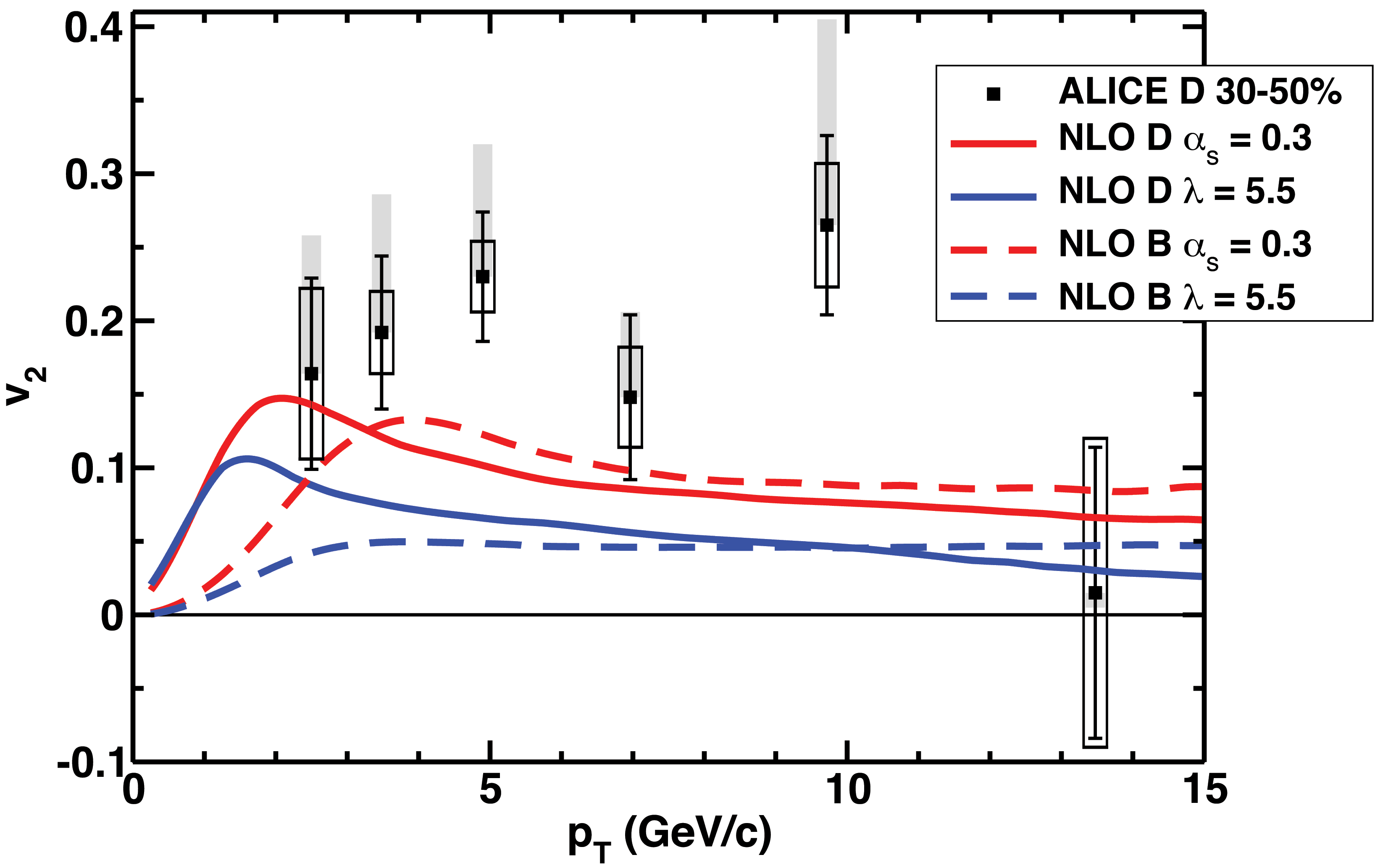
Figure 4: $v_{2}(p_{T})$ for $D$ mesons as measured by ALICE Abelev et al. (2013) at LHC compared to the predictions from the heavy quark energy loss model including fluctuations. For comparison the fluctuating energy loss model predictions for $B$ meson $v_{2}$ are also included. Curves labeled $\alpha_{s}\,=\,0.3$ use $\lambda\,=\,4\pi\times 0.3\times 3$ and $T_{SYM}\,=\,T_{QCD}$; curves labeled $\lambda\,=\,5.5$ have $T_{SYM}\,=\,T_{QCD}/3^{1/4}$.

Ideally, one would very much like some kind of smoking gun experimental measurement to distinguish between weakly-coupled energy loss mechanisms in the plasma compared to strongly-coupled energy loss mechanisms. The double ratio of the nuclear modification factor of $D$ mesons to $B$ mesons was proposed as just such a distinguishing measurement Horowitz and Gyulassy (2008). It was shown in Horowitz and Gyulassy (2008) that the leading order drag prediction for the double ratio is flat as a function of $p_{T}$ and at a value of approximately $m_{D}/m_{B}\,\simeq\,0.2$. On the other hand, pQCD-based energy loss models predict an insensitivity to the mass of the heavy quark when $p_{T}\,\gg\,M_{Q}$, and thus the double ratio starts around 0.2 for $p_{T}\,\sim\,10$ GeV/c and approaches 1 from below by $p_{T}\,\sim\,100$ GeV/c. It is natural to ask whether the strong-coupling prediction for the double ratio of $D$ to $B$ meson nuclear modification factors is affected by the inclusion of fluctuations. It is shown in Fig. 5 that fluctuations completely change the prediction for strong-coupling: the extremely rapid rise in $R_{AA}(p_{T})$ for $D$ mesons due to fluctuations is reflected in an extremely rapid rise in the double ratio, with the double ratio actually going above 1 at $p_{T}\,\sim\,7$ GeV/c. Of course it is precisely at this momentum range that the drag calculation is breaking down; an improved calculation that includes the additional Larmor-like energy loss and autocorrelations in the fluctuations will bring down the double ratio prediction, although it is not yet clear by how much. It seems likely that, for single particle observables, the best experimental measurement to distinguish between heavy quark drag-like energy loss and pQCD-like energy loss will come from $B$ meson $R_{AA}(p_{T})$ alone: Fig. 3 (LABEL:sub@subfig:LHCBJpsi) shows the drag (with fluctuations) prediction decreases significantly with $p_{T}$ and remains relatively constant while pQCD predicts that the $B$ meson $R_{AA}(p_{T})$ will rise as a function of momenta for $p_{T}\,\gtrsim\,25$ GeV/c. One might notice that there is no prediction for $R_{AA}^{B\rightarrow J/\psi}(N_{part})$ given in this work. Since the strong-coupling energy loss model qualitatively describes the most central nuclear modification factor for non-prompt $J/\psi$ mesons, and the model necessarily will predict that the nuclear modification factor goes to unity as collisions become more peripheral, it is difficult to imagine that the energy loss model will not follow the experimentally measured trend Collaboration (2013).

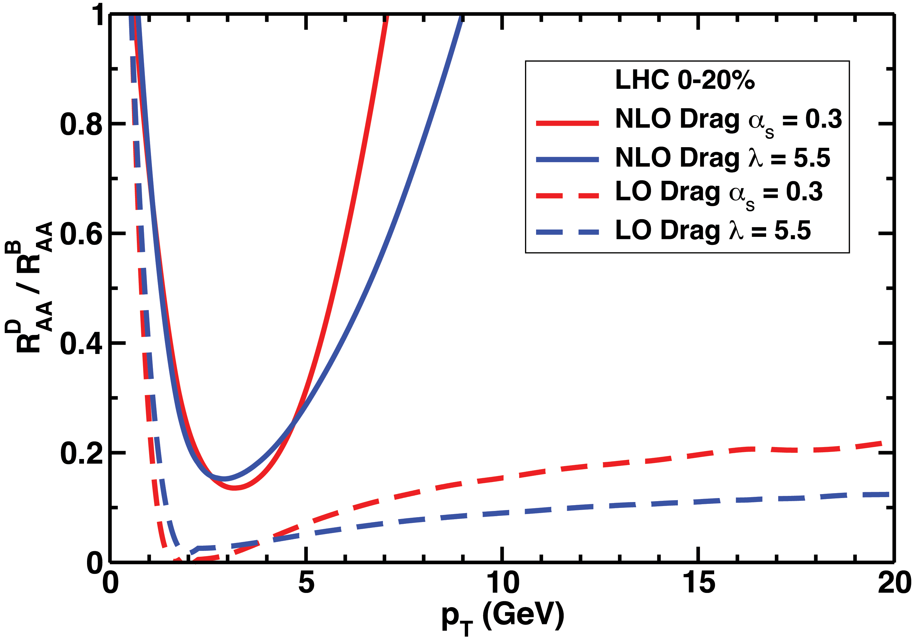
Figure 5: The ratio of $D$ meson $R_{AA}(p_{T})$ to $B$ meson $R_{AA}(p_{T})$ from the strongly-coupled heavy quark energy loss model at leading order (dashed) and including fluctuations (solid). Curves labeled $\alpha_{s}\,=\,0.3$ use $\lambda\,=\,4\pi\times 0.3\times 3$ and $T_{SYM}\,=\,T_{QCD}$; curves labeled $\lambda\,=\,5.5$ have $T_{SYM}\,=\,T_{QCD}/3^{1/4}$.

V Conclusions and Outlook

Hard probes, and, in particular, heavy quarks, provide a crucial test of our theoretical understanding of the physics of quark-gluon plasma. Previous work Horowitz (2012) that included only the leading order energy loss Gubser (2006); Herzog et al. (2006); Casalderrey-Solana and Teaney (2006) for heavy quarks strongly-coupled to a strongly-coupled plasma as calculated from the AdS/CFT correspondence showed significant, falsified disagreement with data Adare et al. (2007); Abelev et al. (2012). The results presented in this paper in Figs. 3 and 4, for which energy loss fluctuations Gubser (2008) are correctly included for the first time in a realistic strong-coupling energy loss model for heavy quarks, are qualitatively consistent with data from RHIC Adare et al. (2011); Mustafa (2013) to LHC Abelev et al. (2012); Chatrchyan et al. (2012); Abelev et al. (2013) within the regime of applicability of the energy loss formulae, Eqs. (1) – (6).

Along with the recent improvement in the treatment of light flavor energy loss in AdS/CFT Morad and Horowitz (2014), in which very good agreement between the suppression of jets from strong-coupling and the preliminary CMS data Collaboration (2012) was shown, strong-coupling can now explain within a self-consistent picture of quark-gluon plasma dynamics a wide and impressive array of observables from low-momentum to high-momentum that includes the rapid applicability of hydrodynamics Chesler and Yaffe (2011), the very small shear viscosity-to-entropy ratio Gubser et al. (1996); Kovtun et al. (2005), the light flavor jet suppression Morad and Horowitz (2014), and the suppression of decay products of heavy quarks (this work).

From the specific perspective of heavy flavor energy loss from AdS/CFT, the next steps include further testing theoretical predictions against data—especially in comparison with predictions from pQCD—and in improving the theory itself.

Surprisingly, as shown in Fig. 5, the inclusion of fluctuations completely changes the leading order Horowitz and Gyulassy (2008) qualitative prediction of the double ratio of $D$ to $B$ nuclear modification factors from the strong-coupling energy loss model: with fluctuations, the double ratio rises rapidly as a function of meson momentum, broaching unity at a momentum scale somewhat above where the calculation is inapplicable due to the speed limit of the setup, Eq. (8). Although the rise is now more rapid than that predicted by pQCD Horowitz and Gyulassy (2008), it is not known how much the momentum rise in the AdS/CFT prediction will be softened as necessary corrections are included to extend the regime of applicability of the calculation to $p_{T}$ above a handful of GeV/c; it is therefore difficult at this stage to use an experimental measurement of the double ratio to test strong- versus weak-coupling physics.

The anisotropy of heavy flavor decay products provides a strong- versus weak-coupling energy loss comparison, although of limited utility. From strong-coupling, as shown in Fig. 4, $B$ meson $v_{2}(p_{T})$ is predicted to be of a similar magnitude to $D$ meson $v_{2}(p_{T})$. Due to mass effects one expects pQCD to predict a smaller anisotropy for $B$ mesons than for $D$ mesons, but it does not seem that predictions for $v_{2}^{B}(p_{T})$ are extant in the literature. This prediction probably has limited use for distinguishing between strong- and weak-coupling dynamics as a precision differentiation of $v_{2}$ for $D$ versus $B$ mesons poses a significant experimental challenge. Additionally, it is not clear the extent to which non-perturbative hadronization effects differ for $D$ versus $B$ meson production in heavy ion collisions at relatively low $\lesssim\,10$ GeV/c momentum at which the AdS/CFT calculations are within their regime of applicability for $D$ mesons.

A likely much more useful prediction comes from the nuclear modification factor of $B$ mesons. As can be seen in Fig. 3 (LABEL:sub@subfig:LHCBJpsi), the strong-coupling energy loss model predicts a large $B$ meson suppression, $R_{AA}(p_{T})\,\sim\,0.1$, out to $p_{T}\,\sim\,30$ GeV/c; in contrast, pQCD predicts a much smaller $B$ meson suppression with $R_{AA}(p_{T})\,\sim\,0.5$ Horowitz (2012). It is worth emphasizing that the strong-coupling energy loss derivations and implementations are under increasing theoretical control as the mass of the quark increases, so future measurements related to $b$ quarks will be especially interesting to see.

Since momentum fluctuations play such an important role in strongly-coupled heavy quark energy loss, and these fluctuations grow characteristically with momentum, a comparison between theory and data related to correlations of pairs of heavy quarks would likely be very enlightening. The comparison would be most meaningful for the decay products of $b$ quarks at high momentum, $10\,\lesssim\,p_{T}\,\lesssim\,100$ GeV/c: above $\sim\,10$ GeV/c any effect that leads to the enhanced $v_{2}$ at intermediate-$p_{T}$ should be small, and one should be able to trust the theoretical calculation below $\sim\,100$ GeV/c. The determination of these correlations from this energy loss model is left for future work.

Improvements to the theoretical calculations that need to be done would increase the regime of applicability of the energy loss formulae and model, thus allowing for a meaningful comparison to more data. The heavy flavor electron predictions could be extended to lower momenta if their production in $p+p$ collisions is brought under better phenomenological control. Both the heavy flavor electron and $D$ meson predictions could be extended to higher momenta if the theoretical and numerical complications related to the speed limit, Eq. (8), could be overcome. It is likely that an entirely different approach to the energy loss calculation, both analytic and numerical, will be required: since the setup of a heavy quark moving at a constant speed is breaking down, presumably one must allow the heavy quark to slow down, which, in turn, will likely mean that full numerical solutions to the worldsheet evolution including thermal fluctuations will be needed. This important, non-trivial research is also left for future work.

Appendix A The Jüttner Distribution

The number of particles $N$ of a relativistic gas in the rest frame of the gas in an $n$-spatial-dimensional box is given by the integral over the invariant phase space of the Jüttner distribution He et al. (2013); Csernai (1994); Cubero et al. (2007), the relativistic generalization of the Maxwell-Boltzmann distribution,

$$N=\int d^{n}x\,d^{n}p\,A\,e^{-p^{0}/T},$$ (16)

in units of $\hbar\,=\,c\,=\,k\,=1$, where $p^{0}\,=\,\surd(\vec{p}^{2}+m^{2})$ is the relativistic energy of a particle of mass $m$, which can be 0. $T$ is the well-defined temperature of the gas in its rest frame, and $A$ is a normalization constant.

Since we are interested in comparing to a numerical simulation with fixed number of particles $N$ we may readily determine $A$:

$$N =A\,V\,\Omega_{n-1}\int_{0}^{\infty}p^{n-1}dp\,e^{-\sqrt{p^{2}+m^{2}}/T},$$ (17)

where

$$\Omega_{d}=\frac{2\pi^{\frac{d+1}{2}}}{\Gamma\big{(}\frac{d+1}{2}\big{)}}$$ (18)

is the volume of a $d$-dimensional sphere; e.g., $\Omega_{2}\,=\,4\pi$. The integral in Eq. (17) may be computed analytically in terms of Gamma and modified Bessel functions, such that

$$A=\frac{1}{2}\frac{N}{V}\Big{(}\frac{m}{2\pi T}\Big{)}^{\frac{n-1}{2}}\frac{1}{m^{n}K_{\frac{n+1}{2}}(m/T)}.$$ (19)

Thus in the rest frame of the plasma the momentum distribution of the $N$ particles is given by

$$\frac{dN}{d^{n}p}=\frac{1}{2}N\Big{(}\frac{m}{2\pi T}\Big{)}^{\frac{n-1}{2}}\frac{e^{-p^{0}/T}}{m^{n}K_{\frac{n+1}{2}}(m/T)}.$$ (20)

Picking out one special direction, say the $z$-direction, one may find the $p^{z}$-differential distribution of particles in the rest frame of the plasma:

$$\frac{dN}{dp^{z}}=\frac{1}{2}N\Big{(}\frac{m}{2\pi T}\Big{)}^{\frac{n-1}{2}}\frac{1}{m^{n}K_{\frac{n+1}{2}}(m/T)}\\ \times\int d^{n-1}p_{T}\,e^{-\sqrt{p_{T}^{2}+(p^{z})^{2}+m^{2}}/T}.$$ (21)

If one is interested in the distribution of particles in a frame that is boosted along, say, the $z$-direction at a speed $\beta$ compared to the rest frame of the plasma, then one finds that in the primed coordinate system

$$\frac{dN}{dp^{z^{\prime}}} =\frac{1}{2}N\Big{(}\frac{m}{2\pi T}\Big{)}^{\frac{n-1}{2}}\frac{1}{m^{n}K_{\frac{n+1}{2}}(m/T)}\int d^{n-1}p_{T}\,\frac{dp^{z}}{dp^{z^{\prime}}}e^{-\sqrt{p_{T}^{2}+\big{(}p^{z}(p^{z^{\prime}})\big{)}^{2}+m^{2}}/T}$$ (22)

$$=\frac{1}{2}N\Big{(}\frac{m}{2\pi T}\Big{)}^{\frac{n-1}{2}}\frac{1}{m^{n}K_{\frac{n+1}{2}}(m/T)}\Omega_{n-2}$$

$$\qquad\times\int p_{T}^{n-2}dp_{T}\,\bigg{(}\frac{\gamma}{\sqrt{p_{T}^{2}+(p^{z^{\prime}})^{2}+m^{2}}}\big{[}\sqrt{p_{T}^{2}+(p^{z^{\prime}})^{2}+m^{2}}-\beta\,p^{z^{\prime}}\big{]}\bigg{)}e^{-\sqrt{p_{T}^{2}+\gamma^{2}\big{(}p^{z^{\prime}}-\beta\sqrt{p_{T}^{2}+(p^{z^{\prime}})^{2}+m^{2}}\big{)}^{2}+m^{2}}/T}$$ (23)

$$=\frac{N\,\gamma^{2}}{\sqrt{2\pi mT}}\Big{(}\frac{m^{2}+(p^{z^{\prime}})^{2}}{\gamma^{2}\,m^{2}}\Big{)}^{n/4}\frac{e^{\gamma\,\beta\,p^{z^{\prime}}/T}}{K_{\frac{n+1}{2}}(m/T)}\Big{(}K_{\frac{n}{2}}\big{(}\gamma\sqrt{(p^{z^{\prime}})^{2}+m^{2}}/T\big{)}-\frac{\beta\,p^{z^{\prime}}}{\sqrt{(p^{z^{\prime}})^{2}+m^{2}}}K_{\frac{n-2}{2}}\big{(}\gamma\sqrt{(p^{z^{\prime}})^{2}+m^{2}}/T\big{)}\Big{)}.$$ (24)

Appendix B Semi-leptonic and $J/\psi$ Fragmentation Functions

The spectrum of electrons $dN^{e}/dp_{T}^{e}(p_{T}^{e})$ (or $J/\psi$ mesons) produced in the lab frame by a spectrum of heavy mesons (in this case a $D$ meson for specificity) that decays into an electron of energy $E$ with probability $P(E)$ in the rest frame of the heavy flavor meson is given by:

$$\frac{dN^{e}}{dp_{T}^{e}}(p_{T}^{e}) =\int dp_{T}^{D}\frac{d\Omega}{4\pi}dE\frac{dN^{D}}{dp_{T}^{D}}(p_{T}^{D})P(E)\delta\Big{(}p_{T}^{e}-E\sqrt{\gamma_{D}^{2}\big{(}\sin(\theta)\cos(\phi)+\beta_{D}\big{)}+\sin^{2}(\theta)\sin^{2}(\phi)}\Big{)}$$ (25)

$$=\int_{p^{D}_{min}}^{\infty}dp_{T}^{D}\int_{\theta_{min}}^{\theta_{max}}\sin(\theta)d\theta\int_{\phi_{min}}^{\phi_{max}}\frac{d\phi}{\pi}J(\theta,\,\phi)\frac{dN^{D}}{dp_{T}^{D}}(p_{T}^{D})P\big{(}p_{T}^{e}\,J(\theta,\,\phi)\big{)}\theta\big{(}|\sec(\theta)|J^{-1}(\theta,\,\phi)-\mathrm{csch}(y_{max})\big{)},$$ (26)

where

$$J(\theta,\,\phi)=\left[\gamma_{D}^{2}\big{(}\sin(\theta)\cos(\phi)+\beta_{D}\big{)}^{2}+\sin^{2}(\theta)\sin^{2}(\phi)\right]^{-1/2},$$ (27)

$$p^{D}_{min} =\mathrm{max}\big{(}0,\,m_{D}\frac{(p_{T}^{e})^{2}-E_{max}^{2}}{2\,p_{T}^{e}\,E_{max}}\big{)}$$

$$\theta_{min} =\mathrm{max}\Big{(}0,\,\mathrm{Re}\big{(}\theta_{crit}^{+}(E_{max})\big{)},\,\mathrm{Re}\big{(}\theta_{crit}^{-}(E_{min})\big{)}\Big{)}$$

$$\theta_{max} =\mathrm{min}\Big{(}\pi/2,\,\mathrm{Re}\big{(}\sin^{-1}(\beta_{D}+p_{T}^{e}/\gamma_{D}\,E_{min})\big{)}\Big{)}$$

$$\phi_{min} =\mathrm{Re}\big{(}\phi_{crit}(E_{min})\big{)}$$

$$\phi_{max} =\mathrm{Re}\big{(}\phi_{crit}(E_{max})\big{)}$$ (28)

$$\theta_{crit}^{\pm}(E) =\sin^{-1}(\mp\beta_{D}\pm p_{T}^{e}/\gamma_{D}E)$$

$$\phi_{crit}(E) =\sin^{-1}\left(\frac{1}{\beta_{D}\sin(\theta)}\Big{(}-1\right.$$

$$\qquad+\left.\sqrt{1-\beta_{D}^{2}-\big{(}\frac{\sin(\theta)}{\gamma_{D}}\big{)}^{2}+\big{(}\frac{p_{T}^{e}}{\gamma_{D}\,E}\big{)}^{2}}\Big{)}\right).$$

$E_{max}$ is the largest energy electron and $E_{min}\,=\,m_{e}$ is the lowest energy electron that can be emitted in a semi-leptonic decay in the rest frame of the heavy meson, and $y_{max}$ is the largest rapidity at which electron measurements are reported (there is an assumption that measurements are restricted symmetrically about $y\,=\,0$). Note that the $\theta$ in the second line of Eq. (25) is the usual Heaviside step function, and

$$\gamma_{D} =\frac{\sqrt{p^{2}+m_{D}^{2}}}{m_{D}}$$ (29)

$$\beta_{D} =\frac{p}{\sqrt{p^{2}+m_{D}^{2}}}.$$ (30)

The explicit probability functions that were used in Eq. (25) are (with some numbers truncated slightly for visibility, although it should not affect results)

$$P^{D\rightarrow e}(E) =(E-E_{min}^{D})(E_{max}^{D}-E)(23.3123E+135.0847E^{2}-685.7559E^{3}+1206.6398E^{4}$$

$$\qquad-1013.2945E^{5}+335.7252E^{6})/1.0015$$ (31)

$$P^{B\rightarrow e}(E) =(E-E_{min}^{B})(E_{max}^{B}-E)(0.0015939-0.002299E+0.069117E^{2}-0.089862E^{3}$$

$$\qquad+0.054773E^{4}-0.012189E^{5})/0.050435$$ (32)

$$P^{B\rightarrow D\rightarrow e}(E) =-0.003556+E(-0.359519+E(27.194146+E(-119.476261+E(244.65394$$

$$\qquad+E(-292.041775+E(218.040963+E(-103.278527+E(30.170577$$

$$\qquad+E(-4.960071+E(0.351141))))))))))(2.65-E)/1.004464$$ (33)

$$P^{B\rightarrow J/\psi}(E) =(E(\sqrt{E^{2}-m_{J/\psi}^{2}}-2)(126.32439(E^{2}-m_{J/\psi}^{2})^{2}+21.848881(E^{2}-m_{J/\psi}^{2})^{3}-$$

$$\qquad 1.728567\sqrt{E^{2}-m_{J/\psi}^{2}}+1.721525(E^{2}-m_{J/\psi}^{2})-64.938832(E^{2}-m_{J/\psi}^{2})^{3/2}$$

$$\qquad-90.585013(E^{2}-m_{J/\psi}^{2})^{5/2}))\Big{/}\big{(}\sqrt{E^{2}-m_{J/\psi}^{2}}E_{m}^{2}(1.728567-1.723872E_{m}+$$

$$\qquad 32.899797E_{m}^{2}-63.517521E_{m}^{3}+51.249069E_{m}^{4}-19.183254E_{m}^{5}+2.731110E_{m}^{6})\big{)},$$ (34)

where $E_{m}\,=\,(m_{B}^{2}-m_{J/\psi}^{2})/2m_{B}$. See Table 1 for the maximum and minimum allowed energies for each of the above $P$ functions.

	$D\rightarrow e$	$B\rightarrow e$	$B\rightarrow D\rightarrow e$	$B\rightarrow J/\psi$
$E_{min}$	$m_{e}$	$m_{e}$	$m_{e}$	$m_{j/\psi}$
$E_{max}$	0.95 GeV	2.3 GeV	2.6 GeV	$\sqrt{E_{m}^{2}+m_{J/\psi}^{2}}$

Table 1: Maximum and minimum allowed energies for the semi-leptonic electron decay fragments of $D$ and $B$ mesons and the $J/\psi$ mesons from $B$ mesons in the rest frame of the decaying heavy meson. $m_{e}\,=\,0.0005$ GeV and $m_{J/\psi}\,=\,3.096916$ GeV.

References

- LRP (2008) “The Frontiers of Nuclear Science, A Long Range Plan,” (2008), arXiv:0809.3137 [nucl-ex] .
- Hirano et al. (2011) Tetsufumi Hirano, Pasi Huovinen, and Yasushi Nara, “Elliptic flow in Pb+Pb collisions at TeV: hybrid model assessment of the first data,” Phys.Rev. C84, 011901 (2011), arXiv:1012.3955 [nucl-th] .
- Shen et al. (2011) Chun Shen, Ulrich Heinz, Pasi Huovinen, and Huichao Song, “Radial and elliptic flow in Pb+Pb collisions at the Large Hadron Collider from viscous hydrodynamic,” Phys.Rev. C84, 044903 (2011), arXiv:1105.3226 [nucl-th] .
- Qiu et al. (2012) Zhi Qiu, Chun Shen, and Ulrich Heinz, “Hydrodynamic elliptic and triangular flow in Pb-Pb collisions at ATeV,” Phys.Lett. B707, 151–155 (2012), arXiv:1110.3033 [nucl-th] .
- Gale et al. (2013) Charles Gale, Sangyong Jeon, Bjorn Schenke, Prithwish Tribedy, and Raju Venugopalan, “Event-by-event anisotropic flow in heavy-ion collisions from combined Yang-Mills and viscous fluid dynamics,” Phys.Rev.Lett. 110, 012302 (2013), arXiv:1209.6330 [nucl-th] .
- Philipsen (2013) Owe Philipsen, “The QCD equation of state from the lattice,” Prog.Part.Nucl.Phys. 70, 55–107 (2013), arXiv:1207.5999 [hep-lat] .
- Majumder and Van Leeuwen (2011) A. Majumder and M. Van Leeuwen, “The Theory and Phenomenology of Perturbative QCD Based Jet Quenching,” Prog.Part.Nucl.Phys. A66, 41–92 (2011), arXiv:1002.2206 [hep-ph] .
- Horowitz (2013) W.A. Horowitz, “Heavy Quark Production and Energy Loss,” Nucl.Phys. A904-905, 186c–193c (2013), arXiv:1210.8330 [nucl-th] .
- Djordjevic et al. (2014) Magdalena Djordjevic, Marko Djordjevic, and Bojana Blagojevic, “RHIC and LHC jet suppression in non-central collisions,” Phys.Lett. B737, 298–302 (2014), arXiv:1405.4250 [nucl-th] .
- Gubser et al. (1996) S.S. Gubser, Igor R. Klebanov, and A.W. Peet, “Entropy and temperature of black 3-branes,” Phys.Rev. D54, 3915–3919 (1996), arXiv:hep-th/9602135 [hep-th] .
- Kovtun et al. (2005) P. Kovtun, Dan T. Son, and Andrei O. Starinets, “Viscosity in strongly interacting quantum field theories from black hole physics,” Phys.Rev.Lett. 94, 111601 (2005), arXiv:hep-th/0405231 [hep-th] .
- Casalderrey-Solana et al. (2011) Jorge Casalderrey-Solana, Hong Liu, David Mateos, Krishna Rajagopal, and Urs Achim Wiedemann, “Gauge/String Duality, Hot QCD and Heavy Ion Collisions,” (2011), arXiv:1101.0618 [hep-th] .
- Chesler and Yaffe (2011) Paul M. Chesler and Laurence G. Yaffe, “Holography and colliding gravitational shock waves in asymptotically AdS5 spacetime,” Phys.Rev.Lett. 106, 021601 (2011), arXiv:1011.3562 [hep-th] .
- Cheng et al. (2008) M. Cheng, N.H. Christ, S. Datta, J. van der Heide, C. Jung, et al., “The QCD equation of state with almost physical quark masses,” Phys.Rev. D77, 014511 (2008), arXiv:0710.0354 [hep-lat] .
- Attems et al. (2013) Maximilian Attems, Anton Rebhan, and Michael Strickland, “Instabilities of an anisotropically expanding non-Abelian plasma: 3D+3V discretized hard-loop simulations,” Phys.Rev. D87, 025010 (2013), arXiv:1207.5795 [hep-ph] .
- Danielewicz and Gyulassy (1985) P. Danielewicz and M. Gyulassy, “Dissipative Phenomena in Quark Gluon Plasmas,” Phys.Rev. D31, 53–62 (1985).
- Horowitz and Gyulassy (2011) W.A. Horowitz and M. Gyulassy, “Quenching and Tomography from RHIC to LHC,” J.Phys. G38, 124114 (2011), arXiv:1107.2136 [hep-ph] .
- Horowitz (2012) W.A. Horowitz, “Testing pQCD and AdS/CFT Energy Loss at RHIC and LHC,” AIP Conf.Proc. 1441, 889–891 (2012), arXiv:1108.5876 [hep-ph] .
- Haque et al. (2014) Najmul Haque, Aritra Bandyopadhyay, Jens O. Andersen, Munshi G. Mustafa, Michael Strickland, et al., “Three-loop HTLpt thermodynamics at finite temperature and chemical potential,” JHEP 1405, 027 (2014), arXiv:1402.6907 [hep-ph] .
- Kurkela and Lu (2014) Aleksi Kurkela and Egang Lu, “Approach to Equilibrium in Weakly Coupled Non-Abelian Plasmas,” Phys.Rev.Lett. 113, 182301 (2014), arXiv:1405.6318 [hep-ph] .
- Gubser (2008) Steven S. Gubser, “Momentum fluctuations of heavy quarks in the gauge-string duality,” Nucl.Phys. B790, 175–199 (2008), arXiv:hep-th/0612143 [hep-th] .
- Casalderrey-Solana and Teaney (2007) Jorge Casalderrey-Solana and Derek Teaney, “Transverse Momentum Broadening of a Fast Quark in a N=4 Yang Mills Plasma,” JHEP 0704, 039 (2007), arXiv:hep-th/0701123 [hep-th] .
- D’Eramo et al. (2011) Francesco D’Eramo, Hong Liu, and Krishna Rajagopal, “Transverse Momentum Broadening and the Jet Quenching Parameter, Redux,” Phys.Rev. D84, 065015 (2011), arXiv:1006.1367 [hep-ph] .
- Casalderrey-Solana et al. (2014) Jorge Casalderrey-Solana, Doga Can Gulhan, José Guilherme Milhano, Daniel Pablos, and Krishna Rajagopal, “A Hybrid Strong/Weak Coupling Approach to Jet Quenching,” (2014), arXiv:1405.3864 [hep-ph] .
- Morad and Horowitz (2014) R. Morad and W.A. Horowitz, “Strong-coupling Jet Energy Loss from AdS/CFT,” JHEP 1411, 017 (2014), arXiv:1409.7545 [hep-th] .
- Collaboration (2012) CMS Collaboration (CMS), “Nuclear modification factor of high transverse momentum jets in PbPb collisions at sqrt(sNN) = 2.76 TeV,” (2012).
- Djordjevic et al. (2006) Magdalena Djordjevic, Miklos Gyulassy, Ramona Vogt, and Simon Wicks, “Influence of bottom quark jet quenching on single electron tomography of Au + Au,” Phys.Lett. B632, 81–86 (2006), arXiv:nucl-th/0507019 [nucl-th] .
- Gubser (2006) Steven S. Gubser, “Drag force in AdS/CFT,” Phys.Rev. D74, 126005 (2006), arXiv:hep-th/0605182 [hep-th] .
- Herzog et al. (2006) C.P. Herzog, A. Karch, P. Kovtun, C. Kozcaz, and L.G. Yaffe, “Energy loss of a heavy quark moving through N=4 supersymmetric Yang-Mills plasma,” JHEP 0607, 013 (2006), arXiv:hep-th/0605158 [hep-th] .
- Casalderrey-Solana and Teaney (2006) Jorge Casalderrey-Solana and Derek Teaney, “Heavy quark diffusion in strongly coupled N=4 Yang-Mills,” Phys.Rev. D74, 085012 (2006), arXiv:hep-ph/0605199 [hep-ph] .
- Chesler et al. (2009) Paul M. Chesler, Kristan Jensen, Andreas Karch, and Laurence G. Yaffe, “Light quark energy loss in strongly-coupled N = 4 supersymmetric Yang-Mills plasma,” Phys.Rev. D79, 125015 (2009), arXiv:0810.1985 [hep-th] .
- Ficnar (2012) Andrej Ficnar, “AdS/CFT Energy Loss in Time-Dependent String Configurations,” Phys.Rev. D86, 046010 (2012), arXiv:1201.1780 [hep-th] .
- Horowitz (2010) William A. Horowitz, “Probing the Frontiers of QCD,” (2010), arXiv:1011.4316 [nucl-th] .
- Akamatsu et al. (2009) Yukinao Akamatsu, Tetsuo Hatsuda, and Tetsufumi Hirano, “Heavy Quark Diffusion with Relativistic Langevin Dynamics in the Quark-Gluon Fluid,” Phys.Rev. C79, 054907 (2009), arXiv:0809.1499 [hep-ph] .
- Karch and Katz (2002) Andreas Karch and Emanuel Katz, “Adding flavor to AdS / CFT,” JHEP 0206, 043 (2002), arXiv:hep-th/0205236 [hep-th] .
- Witten (1998) Edward Witten, “Anti-de Sitter space, thermal phase transition, and confinement in gauge theories,” Adv.Theor.Math.Phys. 2, 505–532 (1998), arXiv:hep-th/9803131 [hep-th] .
- Evans (2013) Lawrence C. Evans, An Introduction to Stochastic Differential Equations (American Mathematical Society, 2013).
- Gardiner (2009) Crispin Gardiner, Handbook of Stochastic Methods for Physics, Chemistry, and Natural Sciences, 4th ed. (Springer, 2009).
- van Kampen (2007) N. G. van Kampen, Stochastic Processes in Physics and Chemistry, 3rd ed. (North-Holland Personal Library, 2007).
- Kloeden and Platen (1995) Peter E. Kloeden and Eckhard Platen, Numerical Solution of Stochastic Differential Equations (Springer, 1995).
- He et al. (2013) Min He, Hendrik van Hees, Pol B. Gossiaux, Rainer J. Fries, and Ralf Rapp, “Relativistic Langevin Dynamics in Expanding Media,” Phys.Rev. E88, 032138 (2013), arXiv:1305.1425 [nucl-th] .
- Wong and Zakai (1965) Eugene Wong and Moshe Zakai, “On the convergence of ordinary integrals to stochastic integrals,” Ann.Math.Stat. 36, 1560–1564 (1965).
- Cacciari et al. (1998) Matteo Cacciari, Mario Greco, and Paolo Nason, “The P(T) spectrum in heavy flavor hadroproduction,” JHEP 9805, 007 (1998), arXiv:hep-ph/9803400 [hep-ph] .
- Cacciari et al. (2001) Matteo Cacciari, Stefano Frixione, and Paolo Nason, “The p(T) spectrum in heavy flavor photoproduction,” JHEP 0103, 006 (2001), arXiv:hep-ph/0102134 [hep-ph] .
- Cacciari et al. (2012) Matteo Cacciari, Stefano Frixione, Nicolas Houdeau, Michelangelo L. Mangano, Paolo Nason, et al., “Theoretical predictions for charm and bottom production at the LHC,” JHEP 1210, 137 (2012), arXiv:1205.6344 [hep-ph] .
- Miller et al. (2007) Michael L. Miller, Klaus Reygers, Stephen J. Sanders, and Peter Steinberg, “Glauber modeling in high energy nuclear collisions,” Ann.Rev.Nucl.Part.Sci. 57, 205–243 (2007), arXiv:nucl-ex/0701025 [nucl-ex] .
- Press et al. (2007) William H. Press, Saul A. Teukolsky, William T. Vetterling, and Brian P. Flannery, Numerical Recipes 3rd Edition: The Art of Scientific Computing (Cambridge University Press, 2007).
- (48) Helmut G. Katzgraber, “Random Numbers in Scientific Computing: An Introduction,” arXiv:1005.4117 [physics.comp-ph] .
- (49) http://www.lpthe.jussieu.fr/~cacciari/fonll/fonllform.html.
- Cacciari et al. (2005) Matteo Cacciari, Paolo Nason, and Ramona Vogt, “QCD predictions for charm and bottom production at RHIC,” Phys.Rev.Lett. 95, 122001 (2005), arXiv:hep-ph/0502203 [hep-ph] .
- (51) Ramona Vogt and Matteo Cacciari, “private communication,” .
- Adare et al. (2011) A. Adare et al. (PHENIX Collaboration), “Heavy Quark Production in and Energy Loss and Flow of Heavy Quarks in Au+Au Collisions at GeV,” Phys.Rev. C84, 044905 (2011), arXiv:1005.1627 [nucl-ex] .
- Mustafa (2013) Mustafa Mustafa (STAR Collaboration), “Measurements of Non-photonic Electron Production and Azimuthal Anisotropy in and 200 GeV Au+ Au Collisions from STAR at RHIC,” Nucl.Phys. A904-905, 665c–668c (2013), arXiv:1210.5199 [nucl-ex] .
- Abelev et al. (2012) Betty Abelev et al. (ALICE), “Suppression of high transverse momentum D mesons in central Pb-Pb collisions at TeV,” JHEP 1209, 112 (2012), arXiv:1203.2160 [nucl-ex] .
- Chatrchyan et al. (2012) Serguei Chatrchyan et al. (CMS), “Suppression of non-prompt , prompt , and Y(1S) in PbPb collisions at TeV,” JHEP 1205, 063 (2012), arXiv:1201.5069 [nucl-ex] .
- Mikhailov (2003) Andrei Mikhailov, “Nonlinear waves in AdS / CFT correspondence,” (2003), arXiv:hep-th/0305196 [hep-th] .
- Fadafan et al. (2009) Kazem Bitaghsir Fadafan, Hong Liu, Krishna Rajagopal, and Urs Achim Wiedemann, “Stirring Strongly Coupled Plasma,” Eur.Phys.J. C61, 553–567 (2009), arXiv:0809.2869 [hep-ph] .
- Abelev et al. (2013) B. Abelev et al. (ALICE Collaboration), “D meson elliptic flow in non-central Pb-Pb collisions at = 2.76TeV,” Phys.Rev.Lett. 111, 102301 (2013), arXiv:1305.2707 [nucl-ex] .
- Shuryak (2002) E.V. Shuryak, “The Azimuthal asymmetry at large p(t) seem to be too large for a ‘jet quenching’,” Phys.Rev. C66, 027902 (2002), arXiv:nucl-th/0112042 [nucl-th] .
- Horowitz (2006) W.A. Horowitz, “Large observed v(2) as a signature for deconfinement,” Acta Phys.Hung. A27, 221–225 (2006), arXiv:nucl-th/0511052 [nucl-th] .
- Aad et al. (2012) Georges Aad et al. (ATLAS Collaboration), “Measurement of the pseudorapidity and transverse momentum dependence of the elliptic flow of charged particles in lead-lead collisions at TeV with the ATLAS detector,” Phys.Lett. B707, 330–348 (2012), arXiv:1108.6018 [hep-ex] .
- Horowitz and Gyulassy (2008) W.A. Horowitz and M. Gyulassy, “Heavy quark jet tomography of Pb + Pb at LHC: AdS/CFT drag or pQCD energy loss?” Phys.Lett. B666, 320–323 (2008), arXiv:0706.2336 [nucl-th] .
- Collaboration (2013) CMS Collaboration, “Prompt and non-prompt with 150 integrated PbPb luminosity at TeV,” CMS-PAS-HIN-12-014 (2013).
- Adare et al. (2007) A. Adare et al. (PHENIX), “Energy Loss and Flow of Heavy Quarks in Au+Au Collisions at s(NN)**(1/2) = 200-GeV,” Phys.Rev.Lett. 98, 172301 (2007), arXiv:nucl-ex/0611018 [nucl-ex] .
- Csernai (1994) L.P. Csernai, Introduction to relativistic heavy ion collisions (1994).
- Cubero et al. (2007) David Cubero, Jesús Casado-Pascual, Jörn Dunkel, Peter Talkner, and Peter Hänggi, “Thermal equilibrium and statistical thermometers in special relativity,” Phys. Rev. Lett. 99, 170601 (2007).