Reflective Network Tomography
Based on Compressed Sensing

Abstract

Network tomography means to estimate internal link states from end-to-end path measurements. In conventional network tomography, to make packets transmissively penetrate a network, a cooperation between transmitter and receiver nodes is required, which are located at different places in the network. In this paper, we propose a reflective network tomography, which can totally avoid such a cooperation, since a single transceiver node transmits packets and receives them after traversing back from the network. Furthermore, we are interested in identification of a limited number of bottleneck links, so we naturally introduce compressed sensing technique into it. Allowing two kinds of paths such as (fully) loopy path and folded path, we propose a computationally-efficient algorithm for constructing reflective paths for a given network. In the performance evaluation by computer simulation, we confirm the effectiveness of the proposed reflective network tomography scheme.

I Introduction

Tomography refers to the cross-sectional imaging of an object from either transmission or reflection data collected by illuminating the object from many different directions [1]. When the object is an information network, it is called network tomography [2], which has been used to encompass a class of approaches to infer the internal link states from end-to-end path measurements [3]. The end-to-end path behaviors have been transmissively measured via a cooperation between transmitter and receiver nodes, which are located at different places in a network. However if it is possible to eliminate such a cooperation, network tomography would become a more powerful method with special properties (implementability, adaptability and asynchronism) for measuring and analyzing network specific characteristics.

In this paper, according to the types of end-to-end path measurements acquisition, we first classify network tomography into transmissive and reflective network tomography, and after discussing their characteristics, we propose a new reflective network tomography scheme. Here, in the reflective network tomography scheme, we focus only on identification of a limited number of links with large delays in a network, where such links are referred to as bottleneck links. In this scheme, a node acts as both a transmitter and a receiver, i.e., as a transceiver: it transmits multiple packets over a network along pre-determined different paths and receives the packets after they traverse back from the network. On the other hand, network tomography is formulated as an undetermined linear inverse problem and it cannot be always solved. However, the assumption in the bottleneck link identification makes it possible to use compressed sensing technique. To propose the new reflective network tomography scheme, we tackle two problems: how to formulate the tomography scheme and how to determine going around paths from/to a transceiver node.

Note that, although end-to-end path measurements can be conducted either actively or passively, reflective network tomography scheme is only based on active measurements. Thus, we particularly consider active tomographic scheme in this paper.

II Network Tomography

II-A Transmissive Network Tomography

In this subsection we define transmissive network tomography via some examples [7, 6, 8, 4, 5, 9] which are characterized by transmissive end-to-end path measurements. Fig. 1 shows an example of a transmissive end-to-end path measurement [4].

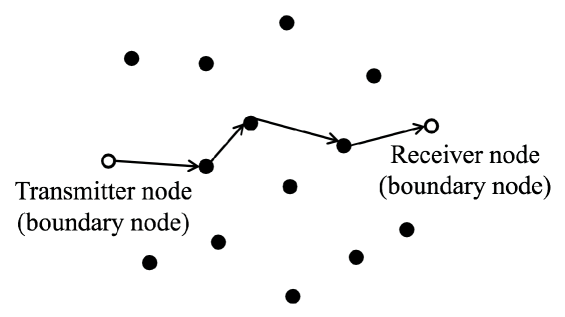
Figure 1: Transmissive end-to-end path measurement.

In a network with a defined boundary, it is assumed that access is available to nodes at the boundary, but not to any in the interior. In order to get transmissive end-to-end path measurements, some boundary nodes are selected as transmitter and receiver nodes. For example, in [4], two nodes are respectively assigned as a transmitter and a receiver, whereas in [5], there are many transmitter and receiver nodes. The transmitter nodes send probe packets to all (or a subset of) the receiver nodes to measure packet attributes on the paths between them. Accordingly, each probe packet transmissively penetrates the network along a measurement path, and brings a transmissive end-to-end path measurement. In [6], a transmissive tomographic methodology based on unicast communication is proposed. In [7] and [8], on the other hand, a single-source multicast transmission by a single or multiple transmitter nodes is applied to networks with tree and general topologies, respectively. From such transmissive end-to-end path measurements between transmitter and receiver nodes, the internal network states such as link-level network parameters can be estimated. For example, in [9], link delay variance is estimated from transmissive end-to-end path measurements in a multicast setting.

II-B Reflective Network Tomography

Unlike transmissive network tomography, reflective network tomography eliminates the need for special-purpose cooperation from receiver nodes. Namely, an end-to-end path measurement is calculated from records on only one node. A boundary node is selected as a transceiver node, and it injects probe packets into the network. Each probe packet goes and back to the transceiver node along a different measurement path, and brings reflective end-to-end path measurements. For example, in [10], a reflective network tomography scheme based on round trip time (RTT) measurement only along a folded path (see IV-B for its definition) is proposed to estimate the delay variance for a link of interest. Thus, in contrast to transmissive network tomography, reflective network tomography is defined by reflective end-to-end path measurements.

III Properties of Reflective Network Tomography

III-A Implementability

The methods described in the above transmissive network tomography all require a coordination between transmitter and receiver nodes. However, the following problems have not been discussed deeply: how to access all the transmitter and receiver nodes and how to establish the coordination between them, in order to implement the network tomography, i.e., designate the measurement paths, transmit active probe packets and collect the end-to-end path measurements. In a network, these would occupy some part of the time/frequency resource and consume some energy. Without any solution strategy, these problems would limit the scope of the paths over which the measurements can be made. Thus most of them would not be widely applicable because of the lack of an available widespread infrastructure for transmissive end-to-end path measurements.

On the other hand, the reflective network tomography scheme does not require special cooperation from the other interior and boundary nodes, because the reflective end-to-end path measurements are calculated only by a single transceiver node. We just use the transceiver node to implement the reflective network tomography, so we can say that the reflective network tomography can be carried out more easily.

III-B Adaptability

Most of the existing transmissive network tomography schemes are based on non-adaptive measurements in themselves. Namely, the measurement paths are often fixed in advance and do not depend on the previously acquired measurements. The reason is that it is difficult to feed back the prior end-to-end path measurements from receiver nodes to transmitter nodes every probing.

In the reflective network tomography scheme, on the other hand, since the probe packets return to the transceiver node, measurement paths can be adaptively selected depending on the previously gathered information. So it can give us the advantage of sequential measuring schemes that adapt to network states using information gathered throughout a measurement period. Furthermore, many current methodologies usually assume that network states are stationary throughout the tomography period. Even when this assumption is not satisfied, however, reflective network tomography scheme may be workable thanks to its adaptability.

III-C Asynchronism

When focusing on transmissive delay tomography which is transmissive network tomography for link delays, end-to-end path measurements are usually calculated from the transmission time and reception time reported by the transmitter and receiver nodes, respectively. Therefore, it requires clock synchronization between them. However, the clock synchronization is sometimes hard to achieve or not guaranteed, especially in wireless networks such as wireless sensor networks, in which electronic components of nodes are too untrustable to meet the requirement of clock synchronization in terms of accuracy and complexity [11, 12]. So, although delay tomography scheme workable in clock-asynchronous networks is preferable, to the best of the authors’ knowledge, the transmissive synchronization-free network tomography has been studied only in [13].

On the other hand, reflective network tomography scheme does not require any clock synchronization for any other nodes in a network. The time delay for a packet traveling through a measurement path can be estimated by checking the transmission time and reception time on a transceiver node’s clock. Therefore, the reflective network tomography scheme is potentially available in clock-asynchronous networks.

IV Proposed Reflective Network Tomography Scheme

IV-A Compressed Sensing

Compressed sensing is an effective theory in signal/image processing for reconstructing a finite-dimensional sparse vector based on its linear measurements of dimension smaller than the size of the unknown sparse vector [14, 15]. Recently, compressed sensing has been also used for network tomography [16, 4, 5]. In this subsection, as the preliminary for compressed sensing, we give several definitions.

First, we define the $\ell_{p}$ norm ($p\geq 1$) of a vector $\mathbf{x}=[x_{1}~{}x_{2}~{}\cdots~{}x_{J}]^{\top}\in\mathcal{R}^{J}$ as

$$\|\mathbf{x}\|_{p}=\Bigl{(}\sum_{i=1}^{J}|x_{i}|^{p}\Bigr{)}^{\frac{1}{p}},$$ (1)

where $\top$ denotes the transpose operator.

Next, we assume that, through a matrix $\mathbf{A}\in\mathcal{R}^{I\times J}$ ($I<J$), we obtain a linear measurement vector $\mathbf{y}=[y_{1}~{}y_{2}~{}\cdots~{}y_{I}]^{\top}\in\mathcal{R}^{I}$ for a vector $\mathbf{x}=[x_{1}~{}x_{2}~{}\cdots~{}x_{J}]^{\top}\in\mathcal{R}^{J}$ as $\mathbf{y}=\mathbf{A}\mathbf{x}$. Whether or not one can recover a sparse vector $\mathbf{x}$ from $\mathbf{y}$ by means of compressed sensing can be evaluated by the mutual coherence $\mu(\mathbf{A})$ [15]. To calculate the mutual coherence of $\mathbf{A}$, by picking up the j-th and j’-th column vectors from $\mathbf{A}$ we construct the partial matrix as

$$\mathbf{A}_{jj^{\prime}}=[\mathbf{c}_{j}~{}\mathbf{c}_{j^{\prime}}],$$ (2)

where $\mathbf{c}_{j}$ and $\mathbf{c}_{j^{\prime}}$ are the $j$-th and $j^{\prime}$-th column vectors of $\mathbf{A}$, respectively. The mutual coherence $\mu(\mathbf{A})$ is defined as the maximum value of $\nu(\mathbf{A}_{jj^{\prime}})$ ($1\leq j,j^{\prime}\leq J,j\neq j^{\prime}$):

$$\mu(\mathbf{A}) = \max_{1\leq j,j^{\prime}\leq J,j\neq j^{\prime}}\nu(\mathbf{A}_{jj^{\prime}}),$$ (3)

$$\nu(\mathbf{A}_{jj^{\prime}}) = \frac{|\mathbf{c}_{j}^{\top}\mathbf{c}_{j^{\prime}}|}{\|\mathbf{c}_{j}\|_{2}\|\mathbf{c}_{j^{\prime}}\|_{2}}.$$ (4)

If

$$k<\frac{1}{2}\Bigl{(}1+\frac{1}{\mu(\mathbf{A})}\Bigr{)},$$ (5)

then there exists at most one vector $\mathbf{x}$ with at most k nonzero components that $\mathbf{y}=\mathbf{A}\mathbf{x}$.

TABLE I: Symbols in Algorithm 1

$\mathcal{P}_{{\rm disjoint}}$	Set of node-disjoint paths.
$\overline{\mathcal{P}}_{{\rm disjoint}}$	Set of node-disjoint reverse paths, which are constructed by reversing directions of paths in $\mathcal{P}_{{\rm disjoint}}$
$\mathcal{W}$	Set of definitive measurement paths.
$\mathit{path}^{(a)}+\mathit{path}^{(b)}$	Path connecting $\mathit{path}^{(a)}$ and $\mathit{path}^{(b)}$.
$\mathcal{P}_{{\rm all}}$	Set of all candidates for measurement paths.
$F_{\mu}(\mathbf{A})$	Function which returns the mutual coherence of $\mathbf{A}$ if no column vector equals $\mathbf{0}$, and number greater than $1$ otherwise.
getCostMin($\mathcal{P}$)	Function which returns a path whose cost is the minimum in a path set $\mathcal{P}$.

IV-B System Model

We consider a delay tomographic scheme which identifies a few bottleneck links in an asynchronous network from reflective end-to-end path measurements. Our approach employs unicast communication. Let $\mathcal{G}=(\mathcal{V},\mathcal{E})$ denote an undirected network, where $\mathcal{V}$ is the node set, and $\mathcal{E}\subseteq\mathcal{V}\times\mathcal{V}$ is the link set. Note that $(i,j)\in\mathcal{E}$ implies that $(j,i)\in\mathcal{E}$ since the graph is undirected. We assume that the topology is fixed throughout the measurement period and there is only one transceiver node $s$.

Due to the fact that the overall delay of a path is the sum of the delays of all links belonging to the path, delay tomography problem can be formulated as an inverse problem to recover link delays based on linear measurements. Here, we measure packet traveling times (PTTs) along two kinds of paths by injecting probe packets into the network. One is a (fully) loopy path (LP) defined as the one where any nodes do not appear more than once except for a transceiver node, and the other is a folded path (FP) defined as the one where any nodes appear twice except for a destination node (in other words, an FP is composed of a path from a transceiver node to a destination node and a path from the destination node to the transceiver node along the same undirected curve between them). Fig. 2 shows an example for LP and FP, and we do not consider any path containing partial loops (routing constraint).

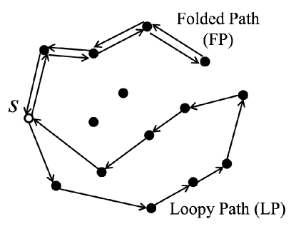
Figure 2: Measuring PTTs based on $s$.

Now, we define $\mathcal{W}=\{\mathit{path}_{s}^{(l)}|~{}l=1,2,\ldots,|\mathcal{W}|\}$ as a subset of all paths to measure PTTs based on $s$, where $\mathit{path}_{s}^{(l)}=\{(s,v^{(l,1)}),(v^{(l,1)},v^{(l,2)}),\ldots,(v^{(l,|\mathit{path}_{s}^{(l)}|-1)},s)\}\subset\mathcal{E}$ represents the $l$-th path in $\mathcal{W}$ and $v^{(l,m)}\in\mathcal{V}\setminus\{s\}$ $(m=1,\ldots,|\mathit{path}_{s}^{(l)}|-1)$ are intermediate nodes in the path.

We reformulate $\mathcal{W}$ and $\mathcal{E}$ as $\mathcal{W}=\{w_{1},w_{2},\ldots,w_{I}\}$ and $\mathcal{E}=\{e_{1},e_{2},\ldots,e_{J}\}$, respectively, where $I=|\mathcal{W}|$ and $J=|\mathcal{E}|$ denote the numbers of paths and links, respectively. We assume that link delays $d_{e_{j}}$ arise independently on each link $e_{j}$ ($j=1,2,\ldots,J$), which does not depend on the direction. Thus, a probe packet transmitted on a path $w_{i}$ ($i=1,2,\ldots,I$) is successfully returned to $s$ with total delay $D_{w_{i}}=\sum_{e_{j}\in w_{i}}d_{e_{j}}$. We define measurement vector $\mathbf{y}=[y_{1}~{}y_{2}~{}\cdots~{}y_{I}]^{\top}$ and link delay vector $\mathbf{x}=[x_{1}~{}x_{2}~{}\cdots~{}x_{J}]^{\top}$ as

$$\begin{split}y_{i}&=D_{w_{i}}=\sum_{e_{j}\in w_{i}}d_{e_{j}},\\ x_{j}&=d_{e_{j}}.\end{split}$$ (6)

Then, we obtain

$$\mathbf{y}=\mathbf{Ax},$$ (7)

where $\mathbf{A}\in\{0,1,2\}^{I\times J}$ represents the (reflective) routing matrix of $\mathcal{W}$, i.e., $(i,j)$-th component $a_{ij}$ ($i=1,2,\ldots,I,~{}j=1,2,\ldots,J$) in $\mathbf{A}$ is set to $a_{ij}=1$ or $a_{ij}=2$ if $e_{j}\in w_{i}$, and $a_{ij}=0$ otherwise. The row size $I$ is related to the interval devoted to the tomography scheme, and the entrywise matrix norm of $\mathbf{A}$

$$\|\mathbf{A}\|=\Bigl{(}\sum_{i=1}^{I}\sum_{j=1}^{J}|a_{ij}|\Bigr{)}$$ (8)

is related to the traffic load of probe packets. The $I$ and $\|\mathbf{A}\|$ determine the energy required for accomplishing a tomography scheme, so the former is referred to as the interval factor, whereas the latter the traffic factor. For a given detectability of bottleneck links, the two factors of a better routing matrix should be smaller.

Note that link states are assumed to be stationary, i.e., link delays do not change while the proposed scheme is applied, and a few bottleneck links exist in the network. Next, because it is possible to approximate the elements of $\mathbf{x}$ corresponding to small link delays to be zero by attributing the delays only to the few bottleneck links, the idea of compressed sensing can be naturally introduced to network tomography. So we utilize compressed sensing based on $\ell_{1}$-$\ell_{2}$ optimization [17, 18] in order to reduce traffic load of probe packets. Finally, when using the PTTs, the assumption of the undirected graph may lead to inaccurate estimates given the asymmetric communication [19]. However, we are interested in identification of a limited number of bottleneck links, thus, the assumption can be considered to be valid, since it does not require measurements with accuracy.

IV-C Routing Matrix Construction

Now, we propose a simple algorithm composed of two steps for constructing a routing matrix $\mathbf{A}$. This algorithm is for a reflective routing matrix which can quickly identify a bottleneck, assuming that a bottleneck link rarely arise in the network. Algorithm 1 shows the algorithm, and Table I describes symbols used in Algorithm 1.

First, in STEP $1$ the algorithm constructs a set of paths as measurement path candidates based on node-disjoint paths algorithm described in [20]. The function NodeDisjointAlgorithm($s$,$v$) in Algorithm 1 returns the maximum set of node-disjoint paths from $s$ to $v$. The set of node-disjoint paths implies the shortest combination of paths where no nodes are shared among the paths. By connecting every node-disjoint path from $s$ to $v$ (for all $v\in\mathcal{V}\setminus s$), this algorithm lists up the candidates for measurement paths, which satisfy the routing constraint that any path is an LP or an FP.

Then, out of the path candidates constructed by STEP 1, STEP $2$ selects paths as measurement paths one-by-one according to the cost of candidates until the mutual coherence of the constructed routing matrix becomes less than 1.0. If several paths have the same minimum cost, the shortest path is selected out of them. Here, we define the cost function for a measurement path ($\mathit{path}\in\mathcal{P}_{{\rm all}}$) as

$$\mbox{Cost}(\mathit{path})$$

$$= \begin{cases}~{}\left(\mbox{Number of unused links in $\mathcal{W}$ out of $\mathit{path}$}\right)^{-1}\\ ~{}~{}~{}~{}~{}~{}~{}~{}~{}~{}~{}~{}~{}~{}~{}~{}~{}~{}~{}~{}~{}~{}~{}~{}~{}~{}~{}~{}~{}~{}~{}~{}~{}\left(\mbox{if }F_{\mu}(\mathbf{A})>1.0\right)\\[6.0pt] \mbox{Number of }\nu(\mathbf{A}^{\prime}_{jj^{\prime}})=1~{}~{}(1\leq j,j^{\prime}\leq J;j\neq j^{\prime})\\ ~{}~{}~{}~{}~{}~{}~{}~{}~{}~{}~{}~{}~{}~{}~{}~{}~{}~{}~{}~{}~{}~{}~{}~{}~{}~{}~{}~{}~{}~{}~{}~{}~{}~{}~{}~{}~{}~{}~{}~{}~{}(\mbox{otherwise}),\end{cases}$$

where $\mathbf{A}^{\prime}$ is constructed from a set $\mathcal{W}+\{\mathit{path}\}$, and this cost function is used in getCostMin($\mathcal{P}$). Once the mutual coherence of the constructed matrix becomes less than 1.0, this algorithm terminates. STEP 2 cannot directly select a path depending on the number of nodes over the path. Therefore, the proposed routing matrix construction algorithm pays attention to the interval factor rather than the traffic factor.

Algorithm 1 Proposed Routing Matrix Construction Algorithm

0:  Network Topology and $s$.

0:  Routing Matrix $\mathbf{A}$.

0:  1 : Search for path candidates

  for all $v\in\mathcal{V}\setminus s$ do

     $\mathcal{P}_{{\rm disjoint}}:={\rm NodeDisjointAlgorithm}(s,v)$.

     for all $\mathit{path}^{(a)}\in\mathcal{P}_{{\rm disjoint}}(a=1,2\cdots|\mathcal{P}_{{\rm disjoint}}|)$ do

        for all $\mathit{path}^{(b)}\in\overline{\mathcal{P}}_{{\rm disjoint}}(b=1,2\cdots|\overline{\mathcal{P}}_{{\rm disjoint}}|)$ do

           $\mathcal{P}_{{\rm all}}:=\mathcal{P}_{{\rm all}}\cup\{\mathit{path}^{(a)}+\mathit{path}^{(b)}\}$.

        end for

     end for

  end for

  2 : Selection of measurement paths

  while  $F_{\mu}(\mathbf{A})\geq 1.0$  do

     $\mathit{path}^{({\rm min})}:={\rm getCostMin}\left(\mathcal{P}_{{\rm all}}\setminus\mathcal{W}\right)$.

     $\mathcal{W}:=\mathcal{W}\cup\{\mathit{path}^{({\rm min})}\}$.

     Construct $\mathbf{A}$ from set $\mathcal{W}$.

  end while

  return  $\mathbf{A}$.

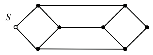
(a) Network topology

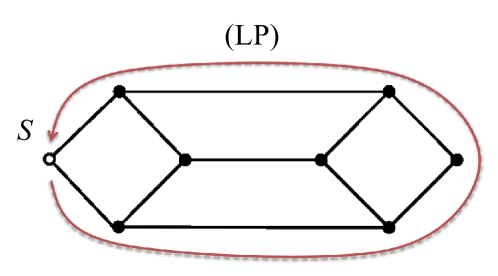
(b) Measurement path ($\mathit{path}_{s}^{(1)}$)

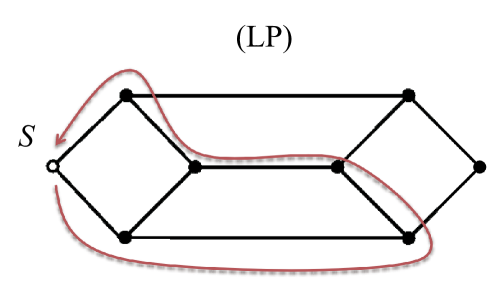
(c) Measurement path ($\mathit{path}_{s}^{(2)}$)

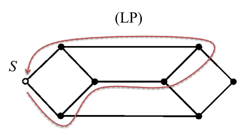
(d) Measurement path ($\mathit{path}_{s}^{(3)}$)

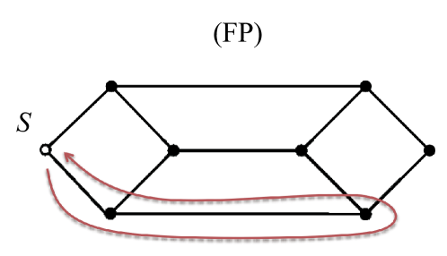
(e) Measurement path ($\mathit{path}_{s}^{(4)}$)

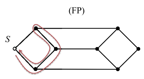
(f) Measurement path ($\mathit{path}_{s}^{(5)}$)

Figure 3: Network topology (8 nodes and 16 links) and the measurement paths constructed by the proposed algorithm.

V Performance Evaluation

In this section, we discuss the following items:

• Can the proposed algorithm (Algorithm 1) construct a fully adequate routing matrix?

• Can a routing matrix constructed by the proposed algorithm actually identify a bottleneck link in a network where only one bottleneck link exists?

• How does a routing matrix with smaller interval and traffic factors behave in a network where several bottleneck links exist?

Fig. 3(a) shows the network topology with $8$ nodes and $11$ links used for performance evaluation by computer simulation, where there is only one transceiver node $s$. We assume that the delay of a bottleneck link is constant with $x^{(B)}$ whereas that of a normal link denoted by $x^{(N)}$ is independent and identically distributed (i.i.d.) with average $\alpha_{x^{(N)}}$ and standard deviation $\sigma_{x^{(N)}}$. In this paper, we also assume that all the nodes are wirelessly connected so $x^{(N)}$ is Gaussian-distributed [21] with $\alpha_{x^{(N)}}=15$ msec and $\sigma_{x^{(N)}}=3$ msec [22, 23].

TABLE II: Routing Matrices

Matrix	Size	Entrywise Matrix Norm	LP:FP Numbers	Number of Candidates
$\mathbf{P}_{1}$	$5\times 11$	$30$	$3:2$	$18$paths
$\mathbf{P}_{2}$	$5\times 11$	$28$	$4:1$	$18$paths
$\mathbf{P}_{3}$	$4\times 11$	$28$	$3:1$	$78$paths

First, Table II shows the constructed three routing matrices whose mutual coherences are less than $1$. In Table II, $\mathbf{P}_{1}$ is constructed by the proposed algorithm composed of STEP 1 and STEP 2 (the measurement paths are shown in Figs. 3(b)-(f)), $\mathbf{P}_{2}$ is constructed by a greedy search from the path candidates listed by STEP 1 (instead of STEP 2, the paths are selected from all combinations of the path candidates by STEP 1, which minimizes the interval and traffic factors), and $\mathbf{P}_{3}$ is also constructed by a greedy search from path candidates listed by STEP 1 and additional FP candidates (all FPs are added to the path candidates by STEP 1 and then the paths are selected from all combinations of the increased path candidates, which minimize the interval and traffic factors). It is impossible for the proposed algorithm to always select the paths which really minimize the interval and traffic factors due to its one-by-one policy (in STEP $2$), on the other hand, the greedy search-based algorithms can always select the optimum set of paths from all combinations of paths. Comparing $\mathbf{P}_{1}$ and $\mathbf{P}_{2}$, the proposed algorithm composed STEP 1 and STEP 2 constructs the routing matrix whose traffic factor is a little larger, and comparing $\mathbf{P}_{2}$ and $\mathbf{P}_{3}$, the number of path candidates by STEP 1 seems insufficient. However, when the size of network is large, for the case where $I$ measurement paths are selected from $N$ candidates, the proposed algorithm calculates the cost function ($IN+I(I-1)/2$) times, whereas the greedy search-based algorithms lead to combinatorial explosion. So, taking into consideration that computational complexity of the proposed algorithm is much lower than that of the greedy search-based algorithm, it can be concluded that the proposed algorithm can efficiently construct a fully adequate routing matrix.

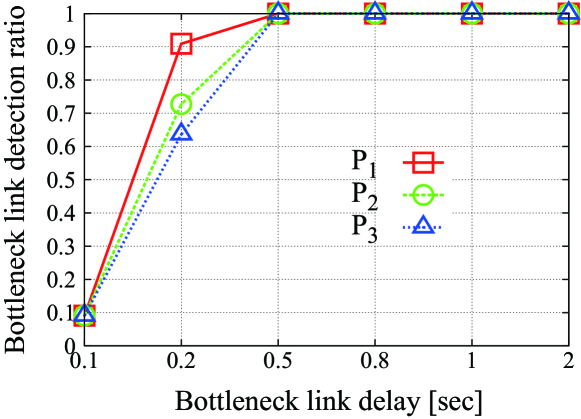
Figure 4: Bottleneck link detection ratio vs. bottleneck link delay $x^{(B)}$ (Number of bottleneck links $k=1$).

The termination of the proposed algorithm is guaranteed since as the number of measurement paths increases, the mutual coherence of the constructed routing matrix monotonously decreases. While mutual coherence can provide a guarantee of the recovery of exactly sparse vectors, the link delay vector $\mathbf{x}$ is approximately sparse in the model for performance evaluation. Therefore, to confirm whether or not the bottleneck link detectability of the reflective network tomography scheme is consistent with the meaning of the mutual coherence. So, we assumed that there is a bottleneck link in the network, that is, we set the number of bottleneck links $k$ to $1$ in the computer simulation. Here, we also define bottleneck link detection ratio which is defined as the number of correctly detected bottleneck links divided by the total number of given bottleneck links. Fig. 4 shows the bottleneck link detection ratio versus the bottleneck link delay for $k=1$. Although the link delay vector $\mathbf{x}$ is not exactly sparse, as the bottleneck link delay $x^{(B)}$ becomes larger, the bottleneck link detection ratios of the three routing matrices approaches $1.0$. This means that, if the bottleneck link delay $x^{(B)}$ is fully larger, the link delay vector $\mathbf{x}$ can be regarded approximately as a sparse vector, and the mutual coherence can also guarantee the recovery of approximately $1$-sparse vectors. Thus, it can be concluded that the proposed scheme can effectively detect a bottleneck link.

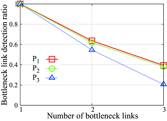
Figure 5: Bottleneck link detection ratio vs. number of bottleneck links $k$ (Bottleneck link delay $x^{(B)}=1.0$).

Finally, we evaluated the matrices $\mathbf{P}_{1},\mathbf{P}_{2},\mathbf{P}_{3}$ in the network with the number of the bottleneck links $k=1,2,3$. Fig. 5 shows the bottleneck link detection ratio versus the number of bottleneck links, where we set $x^{(B)}$ to $1$ sec, which corresponds to about $66.6$ times as large as $\alpha_{x^{(N)}}$. For $k\geq 2$, all the bottleneck link detection ratios fall down sharply. This is because that the algorithms introduced here all try to construct routing matrices with smaller interval and traffic factors, which have worse impact on the bottleneck link detectability of $k\geq 2$ (the proposed algorithm composed of STEP 1 and STEP 2 pays attention only to reducing the interval factor, but it also results in reduction of the traffic factor). Therefore, for a network with the possibility that several bottleneck links arise simultaneously, we need to redesign the termination condition and cost function.

VI Conclusion

In this paper, according to the types of end-to-end path measurements acquisition, we classified network tomography into transmissive and reflective schemes and proposed a new reflective network tomography with their advantageous characteristics over conventional transmissive network tomography. We proposed a simple reflective routing matrix construction algorithms composed of two steps, and by computer simulation we showed that it can effectively construct an adequate routing matrix guaranteeing a designed bottleneck link detectability of $k=1$.

Some technical issues remain in the proposed scheme. First, we have to propose a better routing matrix construction algorithm, and evaluate reflective network tomography on larger networks. We also have to propose an adaptive network tomography to take advantage of reflective characteristic. Since these issues are beyond the scope of this paper, we leave them as future works.

References

- [1] A.C. Kak and M. Slaney, Principles of Computerized Tomographic Imaging. IEEE, 1988.
- [2] Y. Vardi, “Network tomography : estimating source-destination traffic intensities from link data,” J. Amer. Stat. Assoc., vol. 91, no. 433, pp. 365–377, Mar. 1996.
- [3] M. Coates, A.O. Hero III, R. Nowak, and B. Yu, “Internet tomography,” IEEE Signal Process. Mag., vol. 19, no. 3, pp. 47–65, May. 2002.
- [4] K. Takemoto, T. Matsuda, and T. Takine, “Sequential loss tomography using compressed sensing,” IEICE Trans. Commun., vol. E96-B, no. 11, pp. 2756–2765, Nov. 2013.
- [5] M.H. Firooz and S. Roy, “Link delay estimation via expander graphs,” IEEE Trans. Commun., vol. 62, no. 1, pp. 170-181, Jan. 2014.
- [6] M. Coates and R. Nowak, “Network loss inference using unicast end-to-end measurement,” in Proc. ITC Conference on IP Traffic, pp. 28-1–28-9, Sep. 2000.
- [7] R. Cáceres, N.G. Duffield, J. Horowitz, and D.F. Towsley, “Multicast-based inference of network-internal loss characteristics,” IEEE Trans. Inf. Theory, vol. 45, no. 7, pp. 2462–2480, Nov. 1999.
- [8] T. Bu, N. Duffield, F.L. Presti, and D. Towsley, “Network tomography on general topologies,” in Proc. ACM SIGMETRICS, pp. 21–30, Jun. 2002.
- [9] N.G. Duffield and F.L. Presti, “Multicast inference of packet delay variance at interior network links,” in Proc. INFOCOM, pp. 1351–1360, Mar. 2000.
- [10] Y. Tsang, M. Yildiz, P. Barford, and R. Nowak, “Network radar: tomography from round trip time measurements,” in Proc. 4th ACM SIGCOMM Conference on Internet Measurement, pp. 175–180, Oct. 2004.
- [11] B. Sundararaman, U. Buy, and A.D. Kshemkalyani, “Clock synchronization for wireless sensor networks: a survey,” Ad Hoc Networks, vol. 3, no 3, pp. 281–323, May. 2005.
- [12] I.F. Akyildiz, X. Wang, and W. Wang, “Wireless mesh networks: a survey,” Computer Networks, vol. 47, no. 4, pp. 445–487, Mar. 2005.
- [13] K. Nakanishi, S. Hara, T. Matsuda, K. Takizawa, F. Ono, and R. Miura, “Synchronization-free delay tomography based on compressed sensing,” IEEE Commun. Lett., vol. 18, no. 8, pp. 1343–1346, Aug. 2014.
- [14] D.L. Donoho, “Compressed Sensing,” IEEE Trans. Inf. Theory, vol. 52, no. 4, pp. 1289–1306, Apr. 2006.
- [15] Y.C. Eldar and G. Kutyniok, Compressed Sensing: Theory to Applications. Cambridge University Press, 2012.
- [16] W. Xu, E. Mallada, and A. Tang, “Compressive sensing over graphs,” IEEE INFOCOM, pp. 2087–2095, 2011.
- [17] M. Zibulevski and M. Elad, “L1-L2 optimization in signal and image processing,” IEEE Signal Process. Mag., vol. 27, no. 3, pp. 76–88, May 2010.
- [18] T. Matsuda, M. Nagahara, and K. Hayashi, “Link quality classifier with compressed sensing based on - optimization,” IEEE Commun. Lett., vol. 15, no. 10, pp. 1117–1119, Oct. 2011.
- [19] J. Zhao and R. Govindan, “Understanding packet delivery performance in dense wireless sensor networks,” in Proc. the 1st ACM International Conference on Embedded Networked Sensor Systems (SenSys), pp. 1–13, Nov. 2003.
- [20] R. Bhandari, Survivable Networks : Algorithms for Diverse Routing. Springer, 1999.
- [21] K.L. Noh, Q.M. Chaudhari, E. Serpedin, and B.W. Suter, “Novel clock phase offset and skew estimation using two-way timing message exchanges for wireless sensor networks,” IEEE Trans. Commun., vol. 55, no. 4, pp. 766-777, Apr. 2007.
- [22] W. Zeng, X. Chen, Y.A. Kim, and W. Wei, “Delay monitoring for wireless sensor networks: An architecture using air sniffers,” in Proc. IEEE MILCOM., pp. 1–8, Oct. 2009.
- [23] K. Liu, Q. Ma, H. Liu, Z. Cao, and Y. Liu, “End-to-end delay measurement in wireless sensor networks without synchronization,” in Proc. IEEE 10th International Conference on Mobile Ad-Hoc and Sensor Systems (MASS), pp. 583–591, Oct. 2013.