Toward robust early-warning models:
A horse race, ensembles and model uncertainty

Abstract

This paper presents first steps toward robust models for crisis prediction. We conduct a horse race of conventional statistical methods and more recent machine learning methods as early-warning models. As individual models are in the literature most often built in isolation of other methods, the exercise is of high relevance for assessing the relative performance of a wide variety of methods. Further, we test various ensemble approaches to aggregating the information products of the built models, providing a more robust basis for measuring country-level vulnerabilities. Finally, we provide approaches to estimating model uncertainty in early-warning exercises, particularly model performance uncertainty and model output uncertainty. The approaches put forward in this paper are shown with Europe as a playground. Generally, our results show that the conventional statistical approaches are outperformed by more advanced machine learning methods, such as $k$-nearest neighbors and neural networks, and particularly by model aggregation approaches through ensemble learning.

Non-technical summary

The repeated occurrence of financial crises at the turn of the 21st century has stimulated theoretical and empirical work on the phenomenon, not least early-warning models. Yet, the history of these models goes far back. Despite not always referring to macroprudential analysis, the early days of risk analysis relied on assessing financial ratios by hand rather than with advanced statistical methods on computers. During the 1960s, discriminant analysis emerged, being the most dominantly used technique until the 1980s. After the 1980s, DA has mainly been replaced by logit/probit models. Applications of these models range from early models for currency crises to recent ones on systemic financial crises. In parallel, the simple yet intuitive signal extraction approach that simply finds thresholds on individual indicators has gained popularity. With technological advances, a soar in data availability and a thriving need for progress in systemic risk identification, a new group of flexible and non-linear machine learning techniques have been introduced to various forms of financial stability surveillance. Recent literature indicates that these novel approaches hold promise for systemic risk identification because of their ability to identify and map complex dependencies. The premise of difference in performance relates to how methods treat two aspects: individual vs. multiple risk indicators and linear vs. non-linear relationships. While the simplest approaches linearly link individual indicators to crises, the more advanced techniques account for both multiple indicators and different types of non-linearity, such as the mapping of an indicator to crises and interaction effects between multiple indicators.

Despite the fact that some methods hold promise over others, the use and ranking of them is not an unproblematic task. This paper touches upon three problem areas. First, there are few objective and thorough comparisons of conventional and novel methods, and thus neither unanimity on an overall ranking of methods nor on a single best-performing method. Second, given an objective comparison, it is still unclear whether one method can be generalized to outperform others on every single dataset. It is not seldom that different approaches capture different types of vulnerabilities, and hence can be seen to complement each other. Despite potential differences in performance, this would contradict the existence of one single best-in-class method, and instead suggest value in simultaneous use of multiple approaches, or so-called ensembles. Yet, the early-warning literature lacks a structured approach to the use of multiple methods. Third, even if one could identify the best-performing methods and come up with an approach to make use of multiple methods simultaneously, the literature on early-warning models lacks measures of statistical significance or uncertainty. Although crisis probabilities may breach a threshold, there is no work testing the possibility of an exceedance to have occurred due to sampling error alone. Likewise, little or no attention has been given to testing equality of two methods’ early-warning performance or individual probabilities and thresholds.

This paper aims at providing a solution to all of the three above mentioned challenges. First, we conduct an objective horse race of methods for early-warning models, including a large number of common techniques from conventional statistics and machine learning, with a particular focus on the problem as a classification task. The objectivity of the exercise derives from identical sampling into in-sample and out-of-sample data for each method, identical model selection, and identical model specification. For generalizability and comparability, we make use of cross-validation and recursive real-time estimation to assure that and assess how results generalize to out-of-sample data. The two exercises differ in their sampling of data, particularly the in-sample and out-of-sample partitions used for each estimation. While cross-validation is common in machine learning and allows an efficient use of small samples, exercises may benefit from the fact that data are sampled randomly despite most likely exhibiting time dependence. The recursive exercises, on the contrary, account for time dependence in data by strictly using historical samples for out-of-sample predictions, which nevertheless requires more data, particularly in the time-series dimension. These two exercises allow exploring performance across methods, and how that is impacted by the evaluation exercise.

Second, acknowledging the fact that no one method can be generalized to outperform all others, we put forward two strands of approaches for the simultaneous use of multiple methods. A natural starting point is to collect model signals from all methods in the horse race, in order to assess the number of methods that signal for a given country at a given point in time. Two structured approaches involve choosing the best method (in-sample) for out-of-sample use, and relying on the majority vote of all methods together. Then, moving toward more standard ensemble methods for the use of multiple methods, we combine model output probabilities into an arithmetic mean of all methods. With potential further gains in aggregation, we take a performance-weighted mean by letting methods with better in-sample performance contribute more to the aggregated model output. Third, we provide approaches to testing statistical significance in early-warning exercises, including both model performance and output uncertainty. With the sampling techniques of repeated cross-validation and bootstrapping, we estimate properties of the performance of models, and may hence test for statistical significance when ranking models. Further, through sampling techniques, we may also use the variation in model output and thresholds to compute properties for capturing their reliability for individual observations. Beyond confidence bands for representation of uncertainty, this also provides a basis for hypothesis testing, in which an interest of importance ought to be whether a model output is statistically significantly different from the cut-off threshold.

The approaches put forward in this paper are illustrated in a European setting, for which we use a large number of macro-financial indicators for 15 European economies since the 1980s. First, we present rankings of all methods for the objective horse race, after which we proceed to aggregation and statistical significance tests. Generally, our results show that the classical approaches are outperformed by more advanced machine learning methods, such as $k$-nearest neighbors and neural networks, in terms of the Usefulness and Area Under the Curve (AUC) measures. This holds for both horse race exercises. While several of the differences in rankings are statistically insignificant, a particular finding is the outperformance of ensemble models, which is significant in both exercises. More importantly, the objective exercises in this paper provide strong evidence that early-warning modeling in general is a useful tool to identify systemic risk at an early stage.

1 Introduction

Systemic risk measurement lies at the very core of macroprudential oversight, yet anticipating financial crises and issuing early warnings is intrinsically difficult. The literature on early-warning models has, nevertheless, shown that it is no impossible task. This paper provides a three-fold contribution to the early-warning literature: (i) a horse race of early-warning methods, (ii) approaches to aggregating model output from multiple methods, and (iii) model performance and output uncertainty.

The repeated occurrence of financial crises at the turn of the 21st century has stimulated theoretical and empirical work on the phenomenon, not least early-warning models. Yet, the history of these models goes far back. Despite not always referring to macroprudential analysis, the early days of risk analysis relied on assessing financial ratios by hand rather than with advanced statistical methods on computers (e.g., Ramser and Foster [66]). After Beaver’s [9] seminal work on a univariate approach to discriminant analysis (DA), Altman [4] further developed DA for multivariate analysis. Even though DA suffers from frequently violated assumptions like normality of the indicators, it was the dominant technique until the 1980s. Frank and Cline [38] and Taffler and Abassi [83], for example, used DA for predicting sovereign debt crises. After the 1980s, DA has mainly been replaced by logit/probit models. Applications of these models range from the early model for currency crises by Frankel and Rose [39] to a recent one on systemic financial crises by Lo Duca and Peltonen [62]. In parallel, the simple yet intuitive signal extraction approach that simply finds thresholds on individual indicators has gained popularity, again ranging from early work on currency crises by Kaminsky et al. [51] to later work on costly asset booms by Alessi and Detken [1]. Yet, these methods suffer from assumptions violated more often than not, such as fixed distributional relationship between the indicators and the response (e.g., logistic/normal), and the absence of interactions between indicators (e.g., non-linearities in crisis probabilities with increases in fragilities). With technological advances, a soar in data availability and a thriving need for progress in systemic risk identification, a new group of flexible and non-linear machine learning techniques have been introduced to various forms of financial stability surveillance. Recent literature indicates that these novel approaches hold promise for systemic risk identification (e.g., as reviewed in Demyanyk and Hasan [24] and Sarlin [71]). The premise of difference in performance relates to how methods treat two aspects: individual vs. multiple risk indicators and linear vs. non-linear relationships. While the simplest approaches linearly link individual indicators to crises, the more advanced techniques account for both multiple indicators and different types of non-linearity, such as the mapping of an indicator to crises and interaction effects between multiple indicators.

Despite the fact that some methods hold promise over others, the use and ranking of them is not an unproblematic task. This paper touches upon three problem areas. First, there are few objective and thorough comparisons of conventional and novel methods, and thus neither unanimity on an overall ranking of methods nor on a single best-performing method. Though the horse race conducted among members of the Macro-prudential Research Network of the European System of Central Banks aims at a prediction competition, it does not provide a solid basis for objective performance comparisons [3]. Even though disseminating information of models underlying discretionary policy discussion is a valuable task, the panel of presented methods are built and applied in varying contexts. This relates more to a horse show than a horse race. Second, given an objective comparison, it is still unclear whether one method can be generalized to outperform others on every single dataset. It is not seldom that different approaches capture different types of vulnerabilities, and hence can be seen to complement each other. Despite potential differences in performance, this would contradict the existence of one single best-in-class method, and instead suggest value in simultaneous use of multiple approaches, or so-called ensembles. Yet, the early-warning literature lacks a structured approach to the use of multiple methods. Third, even if one could identify the best-performing methods and come up with an approach to make use of multiple methods simultaneously, the literature on early-warning models lacks measures of statistical significance or uncertainty. Moving beyond the seminal work by El-Shagi et al. [33], where the authors put forward approaches for assessing the null of whether or not a model is useful, there is a lack of work estimating statistically significant differences in performance among methods. Likewise, although crisis probabilities may breach a threshold, there is no work testing the possibility of an exceedance to have occurred due to sampling error alone. While Hurlin et al. [47] provide a general-purpose equality test for firms’ risk measures, little or no attention has been given to testing equality of two methods’ early-warning performance or individual probabilities and thresholds.

This paper aims at providing a solution to all of the three above mentioned challenges. First, we conduct an objective horse race of methods for early-warning models, including a large number of common techniques from conventional statistics and machine learning, with a particular focus on the problem as a classification task. The objectivity of the exercise derives from identical sampling into in-sample and out-of-sample data for each method, identical model selection, and identical model specification. For generalizability and comparability, we make use of cross-validation and recursive real-time estimation to assure that and assess how results generalize to out-of-sample data. Rather than an absolute ranking that could be generalized to any context, this provides evidence on the potential in more advanced machine learning approaches in these types of exercises, as well as points to the importance of using appropriate resampling techniques, such as accounting for time dependence. Second, acknowledging the fact that no one method can be generalized to outperform all others, we put forward two strands of approaches for the simultaneous use of multiple methods. A natural starting point is to collect model signals from all methods in the horse race, in order to assess the number of methods that signal for a given country at a given point in time. Two structured approaches involve choosing the best method (in-sample) for out-of-sample use, and relying on the majority vote of all methods together. Then, moving toward more standard ensemble methods for the use of multiple methods, we combine model output probabilities into an arithmetic mean of all methods. With potential further gains in aggregation, we take a performance-weighted mean by letting methods with better in-sample performance contribute more to the aggregated model output. Third, we provide approaches to testing statistical significance in early-warning exercises, including both model performance and output uncertainty. With the sampling techniques of repeated cross-validation and bootstrapping, we estimate properties of the performance of models, and may hence test for statistical significance when ranking models. Further, through sampling techniques, we may also use the variation in model output and thresholds to compute properties for capturing their reliability for individual observations. Beyond confidence bands for representation of uncertainty, this also provides a basis for hypothesis testing, in which an interest of importance ought to be whether a model output is statistically significantly different from the cut-off threshold.

The approaches put forward in this paper are illustrated in a European setting, for which we use a large number of macro-financial indicators for 15 European economies since the 1980s. First, we present rankings of all methods for the objective horse race, after which we proceed to aggregation and statistical significance tests. Generally, our results show that the classical approaches are outperformed by more advanced machine learning methods, such as $k$-nearest neighbors and neural networks, in terms of the Usefulness and Area Under the Curve (AUC) measures. This holds for both horse race exercises. While several of the differences in rankings are statistically insignificant, a particular finding is the outperformance of ensemble models, which is significant in both exercises. More importantly, the objective exercises in this paper provide strong evidence that early-warning modeling in general is a useful tool to identify systemic risk at an early stage.

This paper is organized as follows. In Section 2, we describe the used data, including indicators and events, the methods for the early-warning models, and estimation strategies. Then, we present the set-up for the horse race, as well as approaches for aggregating model output and computing model uncertainty. In Section 4, we present results of the horse race, its aggregations, and model uncertainty in a European setting. Finally, we conclude in Section 5.

2 Data and methods

This section presents the data and methods used in the paper. Whereas the dataset covers both crisis event definitions and vulnerability indicators, the methods include classification techniques ranging from conventional statistical modeling to more recent machine learning algorithms.

2.1 Data

The dataset used in this paper has been collected with the aim of covering as many European economies as possible. While a focus on similar economies might improve homogeneity in early-warning models, we aim at collecting a dataset as large as possible for the data-demanding estimations. The data used in this paper are quarterly and span from 1976Q1 to 2014Q3. The sample is an unbalanced panel with 15 European Union countries: Austria, Belgium, Denmark, Finland, France, Germany, Greece, Ireland, Italy, Luxembourg, the Netherlands, Portugal, Spain, Sweden, and the United Kingdom. In total, the sample includes 15 crisis events, which cover systemic banking crises. The dataset consists of two parts: crisis events and vulnerability indicators. In the following, we provide a more detailed description of the two parts.

Crisis events

The crisis events used in this paper are chosen as to cover country-level distress in the financial sector. We are concerned with banking crises with systemic implications and hence mainly rely on the IMF’s crisis event initiative by Laeven and Valencia [59]. Yet, as their database is partly annual, we complement our events with starting dates from the quarterly database collected by the European System of Central Banks (ESCB) Heads of Research Group, and as reported in Babecky et al. [7]. The database includes banking, currency and debt crisis events for a global set of advanced economies from 1970 to 2012, of which we only use systemic banking crisis events. In general, both of the above databases are a compilation of crisis events from a large number of influential papers, which have been complemented and cross-checked by ESCB Heads of Research. The paper with which the events have been cross-checked include Kindleberger and Aliber [53], IMF [48], Reinhart and Rogoff [67], Caprio and Klingebiel [19], Caprio et al. [20], and Kaminsky and Reinhart [50] among many others.

Early-warning indicators

The second part of the dataset consists of a number of country-level vulnerability indicators. Generally, these cover a range of macro-financial imbalances. We include measures covering asset prices (e.g., house and stock prices), leverage (e.g., mortgages, private loans and household loans), business cycle indicators (GDP and inflation), measures from the EU Macroeconomic Imbalance Procedure (e.g., current account deficits and government debt), and the banking sector (e.g., loans to deposits). In most cases, we have relied on the most commonly used transformation, such as ratios to GDP or income, growth rates, and absolute and relative deviations from a trend. The indicators are sourced from Eurostat, OECD, ECB Statistical Data Warehouse and the BIS Statistics.

For detrending, the trend is extracted using one-sided Hodrick–Prescott filter (HP filter). This means that each point of the trend line corresponds to the ordinary HP trend calculated recursively from the beginning of the series to each point in time. By doing this, we do not use future information when calculating the trend, but rather use the information set available to the policymaker at each point in time. The smoothness parameter of the HP filter is specified to be 400 000 as suggested by Drehmann et al. [25]. This has been suggested to appropriately capture the nature of financial cycles in quarterly data. Growth rates are defined to be annual, whereas we follow Lainà et al. [60] by using both absolute and relative deviations from trend, of which the latter differs from the former by relating the deviation to the value of the trend. The indicators used in this paper combine several sources for broad coverage and for deriving ratios of appropriate variables, and are presented in Table 1. Their descriptive statistics are shown in Table 2.

As proper use of data is essential in order to obtain an objective indication of the usefulness of any modeling approach, a note regarding the relationship between crisis events and indicators is in order. Whilst the uncertainty regarding the definitions of crisis events cannot be disputed, this holds true for any empirical exercise. To visualize the relationship between the actual crisis events and the indicators, as well as their lead time, we include time-series plots for each indicator from $t-12$ to $t+8$ around crisis occurrences in Figure A.1. The figure illustrates that patterns of several indicators, such as the credit gap and asset price changes, for instance, take elevated values prior to crisis events, which is indeed in line with the early-warning literature.

Table 1: A list of indicators.

Table 2: Descriptive statistics of indicators.

2.2 Early warning as a classification problem

Early-warning models require evaluation criteria that account for the nature of the underlying problem, which relates to low-probability, high-impact events. It is of central importance that the evaluation framework resembles the decision problem faced by a policymaker. The signal evaluation framework focuses on a policymaker with relative preferences between type I and II errors, and the usefulness that she derives by using a model, in relation to not using it. In the vein of the loss-function approach proposed by Alessi and Detken [1], the framework applied here follows an updated and extended version in Sarlin [74].

To mimic an ideal leading indicator, we build a binary state variable $C_{n}(h)\in\left\{0,1\right\}$ for observation $n$ (where $n=1,2,\ldots,N$) given a specified forecast horizon $h$. Let $C_{n}(h)$ be a binary indicator that is one during pre-crisis periods and zero otherwise. For detecting events $C_{n}$ using information from indicators, we need to estimate the probability of being in a vulnerable state $p_{n}\in\left[0,1\right]$. Herein, we make use of a number of different methods $m$ for estimating $p_{n}^{m}$, ranging from the simple signal extraction approach to more sophisticated techniques from machine learning. The probability $p_{n}$ is turned into a binary prediction $B_{n}$, which takes the value one if $p_{n}$ exceeds a specified threshold $\tau\in\left[0,1\right]$ and zero otherwise. The correspondence between the prediction $B_{n}$ and the ideal leading indicator $C_{n}$ can then be summarized into a so-called contingency matrix, as described in Table 3.

Table 3: A contingency matrix.

		Actual class $C_{n}$
		Pre-crisis period	Tranquil period
Predicted class $P_{n}$	Signal	Correct call	False alarm
		True positive (TP)	False positive (FP)
	No signal	Missed crisis	Correct silence
		False negative (FN)	True negative (TN)

The frequencies of prediction-realization combinations in the contingency matrix can be used for computing measures of classification performance. A policymaker can be thought to be primarily concerned with two types of errors: issuing a false alarm and missing a crisis. The evaluation framework described below is based upon that in Sarlin [74] for turning policymakers’ preferences into a loss function, where the policymaker has relative preferences between type I and II errors. While type I errors represent the share of missed crises to the frequency of crises $T_{1}\in\left[0,1\right]=$FN/(TP+FN), type II errors represent the share of issued false alarms to the frequency of tranquil periods $T_{2}\in\left[0,1\right]=$FP/(FP+TN). Given probabilities $p_{n}$ of a model, the policymaker then finds an optimal threshold $\tau^{*}$ such that her loss is minimized. The loss of a policymaker includes $T_{1}$ and $T_{2}$, weighted by relative preferences between missing crises ($\mu$) and issuing false alarms ($1-\mu$). By accounting for unconditional probabilities of crises $P_{1}=\mbox{Pr}(C=1)$ and tranquil periods $P_{2}=\mbox{Pr}(C=0)=1-P_{1}$, as classes are not of equal size and errors are scaled with class size, the loss function can be written as follows:

$$L(\mu)=\mu T_{1}P_{1}+(1-\mu)T_{2}P_{2}.$$ (1)

Further, the Usefulness of a model can be defined in a more intuitive manner. First, the absolute Usefulness ($U_{a}$) is given by:

$$U_{a}(\mu)=\mbox{min}(\mu P_{1},\left(1-\mu\right)P_{2})-L(\mu),$$ (2)

which computes the superiority of a model in relation to not using any model. As the unconditional probabilities are commonly unbalanced and the policymaker may be more concerned about the rare class, a policymaker could achieve a loss of $\mbox{min}(\mu P_{1},\left(1-\mu\right)P_{2})$ by either always or never signaling a crisis. This predicament highlights the challenge in building a Useful early-warning model: With a non-perfect model, it would otherwise easily pay-off for the policymaker to always signal the high-frequency class. Second, we can compute the relative Usefulness $U_{r}$ as follows:

$$U_{r}(\mu)=\frac{U_{a}(\mu)}{\mbox{min}(\mu P_{1},\left(1-\mu\right)P_{2})},$$ (3)

where $U_{a}$ of the model is compared with the maximum possible usefulness of the model. That is, the loss of disregarding the model is the maximum available Usefulness. Hence, $U_{r}$ reports $U_{a}$ as a share of the Usefulness that a policymaker would gain with a perfectly-performing model, which supports interpretation of the measure. It is worth noting that $U_{a}$ better lends to comparisons over different $\mu$.

Beyond the above measures, the contingency matrix may be used for computing a wide range of other quantitative measures. Receiver operating characteristics (ROC) curves and the area under the ROC curve (AUC) are also used for comparing performance of early-warning models and indicators. The ROC curve plots, for the complete range of $\tau\in[0,1]$, the conditional probability of positives to the conditional probability of negatives:

$$ROC=\frac{\mbox{Pr}(P=1\mid C=1)}{1-\mbox{Pr}(P=0\mid C=0)}.$$

2.3 Classification methods

The purpose of any classification algorithm is to identify to which of a set of classes a new observation belongs, based on one or more predictor variables. Classification is considered an instance of supervised learning, where a training set of correctly identified observations is available. In this paper, a number of probabilistic classifiers are used, whose outputs are probabilities indicating to which of the qualitative classes an observation belongs. In our case, the dependent (or outcome) variable represents the two classes of pre-crisis periods (1) and tranquil periods (0).

Generally, a classifier attempts to assign each observation to the most likely class, given its predictor values. For the binary case, where there are only two possible classes, an optimal classifier (which minimizes the error rate) predicts class one if $\mbox{Pr}(Y=1|X=x)>0.5$, and class zero otherwise. This classifier is denoted as the Bayes classifier. Ideally, one would like to predict qualitative responses using the Bayes classifier, but for real-world data, however, the conditional distribution of $Y$ given $X$ is unknown. Thus, the goal of many approaches is to estimate this conditional distribution and classify an observation to the category with the highest estimated probability. For real-world applications, it may also be noted that the optimal threshold $\tau$ between classes is not always 0.5, but varies. This optimal threshold may be a result of optimizing the above discussed Usefulness, and is examined in further detail later in the paper.

This paper aims to gather a versatile set of different classification methods, from the simple approach of signal extraction to the considerably more computationally intensive neural networks and support vector machines. The methods used for deriving early-warning models have been put into context in Figure 1 and papers applying these methods in an early-warning exercise have been reviewed in Table 4. The methods are presented in more detail below.

Signal extraction

The signal extraction approach introduced by Kaminsky et al. [51] simply analyzes the level of an indicator, and issues a signal if the value exceeds a specified threshold. In order to issue binary signals, we specify the threshold value as to optimize classification performance, which is herein measured with relative Usefulness [50]. However, the key limitation of this approach is that it does not enable any interaction between or weighting of indicators, while an advantage is that it demonstrates a more direct measure of the importance and provides a ranking of each indicator. Despite this, it is one of the most commonly applied early-warning techniques.

Linear Discriminant Analysis (LDA)

LDA, introduced by Fisher [36], is a commonly used method in statistics for expressing one dependent variable as a linear combination of one or more continuous predictors. LDA assumes that the predictor variables are normally distributed, with a mean vector and a common covariance matrix for all classes, and implements Bayes’ theorem to approximate the Bayes classifier. LDA has been shown to perform well on small data sets, if the above-mentioned conditions apply. Yet even though DA suffers from the frequently violated assumptions, it was the dominant technique until the 1980s, after which it was oftentimes replaced by logit/probit models.

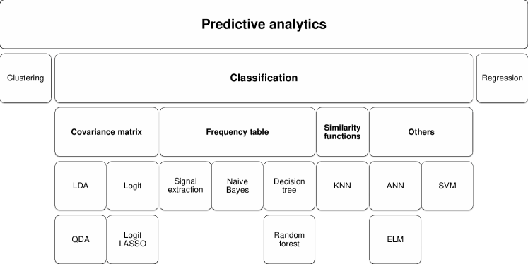
Figure 1: A taxonomy of classification methods

Quadratic Discriminant Analysis (QDA)

QDA is a variant of LDA, which estimates a separate covariance matrix for each class (see, e.g., Venables and Ripley [86]). This causes the number of parameters to estimate to rise significantly, but consequently results in a non-linear decision boundary. To the best of our knowledge, QDA has not been applied for early-warning exercises at the country level.

Logit analysis

Much of the early-warning literature deals with models that rely on logit/probit regression. Logit analysis uses the logistic function to describe the probability of an observation belonging to one of two classes, based on a regression of one or more continuous predictors. For the case with one predictor variable, the logistic function is $p(X)=\frac{e^{\beta_{0}+\beta_{1}X}}{1+e^{\beta_{0}+\beta_{1}X}}$. From this, it is obvious to extend the function to the case of several predictors. Logit and probit models have frequently been applied to predicting financial crises, as can be seen in an early review by Berg et al. [11]. However, the distributional (logistic/normal) assumption on the relationship between the indicators and the response as well as the absence of interactions between variables may often be violated. Lo Duca and Peltonen [62], for example, show that the probability of a crisis increases non-linearly as the number of fragilities increase.

Logit LASSO

The LASSO (Least Absolute Shrinkage and Selection Operator) logistic regression (Tibshirani [84]) attempts to select the most relevant predictor variables for inference and is often applied to problems with a large number of predictors. The method maximizes the log likelihood subject to a bound on the sum of absolute values of the coefficients $\mathrm{max}{}_{\beta}l(\beta\mid y)-\lambda\sum_{i}\mid\beta_{i}\mid$, for which the $\mid\beta_{i}\mid$ is penalized by the $L_{1}$ norm. This implies that the LASSO sets some coefficients to equal zero, and produces sparse models with a simultaneous variable selection. The optimal penalization parameter $\lambda$ is oftentimes chosen empirically via cross-validation. We are only aware of the use of the Logit LASSO in this context in Lang et al. [61], wherein it is mainly used to identify risks in bank-level data, but also aggregated to the country level for assessing risks in entire banking sectors.

Naive Bayes

In machine learning, the Naive Bayes method is one of the most common Bayesian network methods (see e.g. Kohavi et al. [57]). Bayesian learning is based on calculating the probability of each hypothesis (or relation between predictor and response), given the data. The method is called ’naive’ as it assumes that the predictor variables are conditionally independent. Consequently, the method may give high weights to several predictors which are correlated, unlike the methods discussed above, which balance the influence of all predictors. However, the method has been known to scale well to large problems. To the best of our knowledge, Naive Bayes has not been applied for early-warning exercises at the country level.

$k$-nearest neighbors (KNN)

KNN is a non-parametric method which uses similarity functions to determine the class of an observation based on its $k$ nearest observations (see, e.g. Altman [5]). Given a positive integer $k$ and an observation $x_{0}$, the algorithm first identifies the $k$ points $x_{k}$ in the data closest to $x_{0}$. The probability for belonging to a class is then estimated as the fraction of the $k$ closest points, whose response values correspond with the respective class. The method is considered to be among the simplest in the realm of machine learning, and has two free parameters, the integer $k$ and a parameter which affects the search distance for neighbors, which can be optimized for each data set. As with Naive Bayes, we are not aware of previous use of KNN in early-warning exercises at the country level.

Classification trees

Classification trees, as discussed by Breiman et al. [17], implement a decision tree-type structure, which reach a decision by performing a sequence of tests on the values of the predictors. In a classification tree, the classes are represented by leaves, and the conjunctions of predictors are represented by the branches leading to the classes. These conjunction rules segment the predictor space into a number of simpler regions, allowing for decision boundaries of complex shapes. Given similar loss functions, an identical result could also be reached through sequential signal extraction. The method has proven successful in many areas of machine learning, and has the advantage of high interpretability. To reduce complexity and improve generalizability, sections of the tree are often pruned until optimal out-of-sample performance is reached. The degree of pruning is determined by a complexity parameter, which is used in this paper as a free parameter. In the early-warning literature, the use of classification trees has been fairly common.

Random forest

The random forest method, introduced by Breiman [15], uses classification trees as building blocks to construct a more sophisticated method, at the expense of interpretability. The method grows a number of classification trees based on differently sampled subsets of the data. Additionally, at each split, a randomly selected sample is drawn from the full set of predictors. Only predictors from this sample are considered as candidates for the split, effectively forcing diversity in each tree. Lastly, the average of all trees is calculated. As there is less correlation between the trees, this leads to a reduction in variance in the average. In this paper, two free parameters are considered: the number of trees, and the number of predictors sampled as candidates at each split. To the best of our knowledge, random forests have only been applied to early-warning exercises in Alessi and Detken [2].

Artificial Neural Networks (ANN)

Inspired by the functioning of neurons in the human brain, ANNs are composed of nodes or units connected by weighted links (see, e.g., Venables and Ripley [86]). These weights act as network parameters that are tuned iteratively by a learning algorithm. The simplest type of ANN is the single hidden layer feed-forward neural network (SLFN), which has one input, hidden and output layer. The input layer distributes the input values to the units in the hidden layer, whereas the unit(s) in the output layer computes the weighted sum of the inputs from the hidden layer, in order to yield a classifier probability. Despite ANNs with no size restrictions are universal approximators for any continuous function [44], computation time increases exponentially and their interpretability diminishes as ANNs grow in size. Further, discriminant and logit/probit analysis can in fact be related to very simple ANNs [68, 70]: so-called single-layer perceptrons (i.e., no hidden layer) with a threshold and logistic activation function. This paper uses a basic SLFN with three free parameters: the number of units in the hidden layer, the maximum number of iterations, and the weight decay. The first parameter controls the complexity of the network, while the last two are used to control how the learning algorithm converges. The use of ANNs has been fairly common in the academic early-warning literature.

Extreme Learning Machines (ELM)

As introduced by Huang et al. [46], the ELM refers to a specific learning algorithm used to train a SLFN-type neural network. Unlike conventional iterative learning algorithms, the ELM algorithm randomizes the input weights and analytically determines the output weights of the network. When trained with this algorithm, the SLFN generally requires a higher number of units in the hidden layer, but computation time is greatly reduced and the resulting neural network may have better generalization ability. In this paper, two free parameters are considered: the number of units in the hidden layer, and the type of activation function used in the network. To the best of our knowledge, we are not aware of previous applications of the ELM algorithm to crisis prediction.

Support Vector Machines (SVM)

The SVM, introduced by Cortes and Vapnik [23], is one of the most popular machine learning methods for supervised learning. It is a non-parametric method that uses hyperplanes in a high-dimensional space to construct a decision boundary for a separation between classes. It comes with several desirable properties. First, an SVM constructs a maximum margin separator, i.e. the chosen decision boundary is the one with the largest possible distance to the training data points, enhancing generalization performance. Second, it relies on support vectors when constructing this separator, and not on all the data points, such as in logistic regression. These properties lead to the method having high flexibility, but still being somewhat resistant to overfitting. However, SVMs lack interpretability. The free parameters considered are: the cost parameter, which affects the tolerance for misclassified observations when constructing the separator; the gamma parameter, defining the area of influence for a support vector; and the kernel type used. We are not aware of studies using SVMs for the purpose of deriving early-warning models.

Table 4: Literature review.

Method	Currency crisis	Sovereign crisis	Banking crisis
Signal extraction	[51]	[54]	[12] [1]
LDA	–	[38] [83]	–
QDA	–	–	–
Logit	[32] [39] [69] [10] [18]	[80] [40]	[8] [62]
Logit LASSO	–	–	[61]
KNN	–	–	–
Trees	[49] [21]	[79]	[26]
Random forest	–	–	[2]
ANN	[63] [37] [64] [76]	[34]	[71]
ELM	–	–	–
SVM	–	–	–

3 Horse race, aggregation and model uncertainty

This section presents the methodology behind the robust and objective horse race and its aggregation, as well as approaches for estimating model uncertainty.

3.1 Set-up of the horse race

To continue from the data, classification problem and methods presented in Section 2, we herein focus on the set-up for and parameters used in the horse race, ranging from details in the use of data and general specification of the classification problem to estimation strategies and modeling. The aim of the set-up is to mimic real-time use as much as possible by both using data in a realistic manner and tackling the classification problem using state-of-the-art specifications. The specification needs also to be generic in nature, as the objectivity of a horse race relies on applying the same procedures to all methods.

Model specifications

This section describes the choices regarding model specifications that underlie the exercises in this paper. In all choices, we have tried to follow the convention in the most recent literature on the topic. Despite the fact that model output is country-specific, the literature has preferred the use of pooled data and models (e.g., Fuertes and Kalotychou [40], Sarlin and Peltonen [77]). In theory, one would desire to account for country-specific effects describing crises, but the rationale behind pooled models descends from the aim to capture a wide variety of crises and the relatively small number of events in individual countries. Further, as we are interested in vulnerabilities prior to crises and do not lag explanatory variables for this purpose, the benchmark dependent variable is defined as a specified number of years prior to the crisis. In the horse race, the benchmark is 5–12 quarters prior to a crisis.

As proposed by Bussière and Fratzscher [18], we account for post-crisis and crisis bias by not including periods when a crisis occurs or the two years thereafter. The excluded observations are not informative regarding the transition from tranquil times to distress events, as they can neither be considered “normal” periods nor vulnerabilities prior to crises. Following the same reasoning, observations 1–4 quarters prior to crises are also left out. To issue binary signals with method $m$, we need to specify a threshold value $\tau$ on the estimated probabilities $p_{n}^{m}$, which is set as to optimize Usefulness (as outlined in Section 2.2). We assume a policymaker to be more concerned of missing a crisis than giving a false alarm. Hence, the benchmark preference $\mu$ is assumed to be 0.8. This reasoning follows the fact that a signal is treated as a call for internal investigation, whereas significant negative repercussions of a false alarm only descend from external announcements.

For comparability, we consistently transform output probabilities of each method into their own percentile distributions of in-sample data. This is particularly relevant for model aggregation, as it is important for model output to be on the same scale. More specifically, the empirical cumulative distribution function is computed based on the in-sample probabilities for each method, and both the in-sample and out-of-sample probabilities are converted to percentiles of the in-sample probabilities.

Estimation strategies

With the aim of tackling the classification problem at hand, this paper uses two conceptually different estimation strategies. First, we use cross-validation for preventing overfitting and for objective comparisons of generalization performance. Second, we test the performance of methods when applied in the manner of a real-time exercise.

The resampling method of cross-validation, as introduced by Stone [82] in the 1970s, is commonly used in machine learning to assess the generalization performance of a model on out-of-sample data and to prevent overfitting. Out of a range of different approaches to cross-validation, we make use of so-called $K$-fold cross-validation. In line with the famous evidence by Shao [81], leave-one-out cross-validation does not lead to a consistent estimate of the underlying true model, whereas certain kinds of leave-n-out cross-validation are consistent. Further, Breiman [14] shows that leave-one-out cross-validation may also run into trouble with the problem that a small change in the data causes a large change in the model selected, whereas Breiman and Spector [16] and Kohavi [56] found that $K$-fold works better than leave-one-out cross-validation. For an extensive survey article on cross-validation see Arlot and Celisse [6]. Cross-validation is used here in two ways. The first aim of cross-validation is to function as a tool for model selection for obtaining optimal free parameters, with the aim of generalizing data rather than (over)fitting on in-sample data. The other aim relates to objective comparisons of models’ performance on out-of-sample data, given an identical sampling for the cross-validated model estimations. The scheme used herein involves sampling data into $K$ folds for cross-validation and functions as follows:

1. Randomly split the set of observations into $K$ folds of approximately equal size.

2. For the $k\mbox{th}$ out-of-sample validation fold, fit a model to and compute an optimal threshold $\tau^{*}$ using $U_{r}^{K-1}(\mu)$ with the remaining $K-1$ folds, also called the in-sample data. Apply the threshold to the $k\mbox{th}$ fold and collect its out-of-sample $U_{r}^{k}(\mu)$.

3. Repeat Steps 1 and 2 for $k=1,2,...,K$, and collect out-of-sample performance for all $K$ validation sets as $U_{r}^{K}(\mu)=\frac{1}{K}\sum_{k=1}^{K}U_{r}^{k}(\mu)$.

For model selection, a grid search of free parameters is performed for the methods supporting those. As stated previously, $K$-fold cross-validation is used and the free parameters yielding the best performance on the out-of-sample data are stored and applied in subsequent analysis. The literature has generally preferred small values for $K$, with $K=10$ being among the most prominently used number of folds (see e.g. Zhang [88].) The cross-validated horse race makes use of 10-fold cross-validation to provide objective relative assessments of generalization performance of different models. The latter purpose of cross-validation is central for the horse race, as it allows for comparisons of models, and thus different modeling techniques, but still assures identical sampling.

The standard approach to cross-validation may not, however, be entirely unproblematic. As we make use of panel data, including a cross-sectional and time dimension, we should also account for the fact that the data are more likely to exhibit temporal dependencies. Although the cross-validation literature has put forward advanced techniques to decrease the impact of dependence, such as a so-called modified cross-validation by Chu and Marron [22] (further examples in Arlot and Celisse [6]), the most prominent approach is to limit estimation samples to historical data for each prediction. To test models from the viewpoint of real-time analysis, we use a recursive exercise that derives a new model at each quarter using only information available up to that point in time. This enables testing whether the use of a method would have provided means for predicting the global financial crisis of 2007–2008, and how methods are ranked in terms of performance for the task. This involves accounting for publication lags by lagging accounting based measures with 2 quarters and market-based variables with 1 quarter. The recursive algorithm proceeds as follows. We estimate a model at each quarter with all available information up to that point, evaluate the signals to set an optimal threshold $\tau^{*}$, and provide an estimate of the current vulnerability of each economy with the same threshold as on in-sample data. The threshold is thus time-varying. At the end, we collect all probabilities and thresholds, as well as the signals, and evaluate how well the model has performed in out-of-sample analysis. As any ex post assessment, it is crucial to acknowledge that also this exercise is performed in a quasi real-time manner with the following caveats. Given how data providers report data, it is not possible to account for data revisions, and potential changes may hence have occurred after the first release. Moreover, we experiment with two different approaches for real-time use of pre-crisis periods as the dependent variable. With a forecast horizon of three years, we will at each quarter know with certainty only after three years whether or not the current quarter is a pre-crisis period to a crisis event (unless a crisis has occurred in the past three years). We test both dropping a window of equal length as the forecast horizon and using pre-crisis periods for the assigned quarters. As a horse race, the recursive estimations test the models from the viewpoint of real-time analysis. Using in-sample data ranging back as far as possible, the recursive exercise starts from 2005Q2, with the exception of the QDA method, for which analysis starts from 2006Q2, due to requirements of more training data than for the other methods. This procedure enables us to test performance with no prior information on the build-up phase of the recent crisis.

3.2 Aggregation procedures

From individual methods, we move forward to combining the outputs of several different methods into one through a number of aggregation procedures. The approaches here descend from the subfield of machine learning focusing on ensemble learning, wherein the main objective is the use of multiple statistical learning algorithms for better predictive performance. Although we aim for simplicity and do not adopt the most complex algorithms herein, we make use of the two common approaches in ensemble learning: bagging and boosting. Bagging stands for Bootstrap Aggregation [13] and makes use of resampling from the original data, which is to be aggregated into one model output. While being an approach for ensemble learning, we discuss this under the topic of resampling and model uncertainty, as can be seen in Section 3.3. Boosting [78] refers to computing output from multiple models and then averaging the results with specified weights, which we mainly rely on in our aggregation procedures below. A third group of stacking approaches [87], which add another layer of models on top of individual model output to improve performance, are not used in this paper for the sake of simplicity. Again, we use the optimal free parameters identified through cross-validated grid searches, and then estimate individual methods. For this, we make use of four different aggregation procedures: the best-of and voting approaches, and arithmetic and weighted averages of probabilities.

The best-of approach simply makes use of one single method $m$ by choosing the most accurate one. To use information in a truthful manner, we always choose the method, independent of the exercise (i.e., cross-validation or recursion), which has the best in-sample relative Usefulness. Voting simply makes use of the signals $B_{n}^{m}$ of all methods $m=1,2,...,M$ for each observation $x_{n}$ in order to signal or not based upon a majority vote. That is, the aggregate $B_{n}^{a}$ chooses for observation $x_{n}$ the class that receives the largest total vote from all individual methods:

$$B_{n}^{a}=\left\{\begin{array}[]{ccc}1&\mbox{if}&\frac{1}{M}\sum_{m=1}^{M}B_{n}^{m}>0.5\\ 0&\mbox{otherwise}\end{array}\right.,$$

where $B_{n}^{m}$ is the binary output for method $m$ and observation $n$, and $B_{n}^{a}$ is the binary output of the majority vote aggregate.

Aggregating probabilities requires an earlier intervention in modeling. In contrast to the best-of and voting approaches, we directly make use of the probabilities $p_{n}^{m}$ of each method $m$ for all observations $n$ to average them into aggregate probabilities. The simpler case uses an arithmetic mean to derive aggregate probabilities $p_{n}^{a}$. For weighted aggregate probabilities $p_{n}^{a}$, we make use of in-sample model performance when setting the weights of methods, so that the most accurate method (in-sample) is given the most weight in the aggregate. The non-weighted and weighted probabilities $p_{n}^{a}$ for observations $x_{n}$ can be derived as follows:

$$p_{n}^{a}=\sum_{m=1}^{M}\frac{w_{m}}{\sum_{m=1}^{M}w_{m}}p_{j}^{m}$$

where the probabilities $p_{n}^{m}$ of each method $m$ are weighted with its performance measure $w_{m}$ for all observations $n$. In this paper, we make use of weights $w_{m}=U_{r}^{m}(\mu)$, but the approach is flexible for any chosen measure, such as the AUC. This weighting has the property of giving the least useful method the smallest weight, and accordingly a bias towards the more useful ones. The arithmetic mean can be shown to result in $p_{n}^{a}=\frac{1}{M}\sum_{m=1}^{M}p_{n}^{m}$ for $w_{m}=1$. To make use of only available information in a real-time set-up, the $U_{r}^{m}(\mu)$ used for weighting refers always to in-sample results. In order to assure non-negative weights, we drop methods with negative values (i.e., $U_{r}^{m}(\mu)<0$) from the vector of performance measures. In the event that all methods show a negative Usefulness, they are given weights of equal size. After computing aggregate probabilities $p_{n}^{a}$, they are treated as if they were outputs for a single method (i.e., $p_{n}^{m}$), and optimal thresholds $\tau^{*}$ identified accordingly. In contrast, the best-of approach signals based upon the identified individual method and voting signals if and only if a majority of the methods signal, which imposes no requirement of a separate threshold. Thus, the overall cross-validated Usefulness of the aggregate is calculated in the same manner as for individual methods. Likewise, for the recursive model, the procedure is identical, including the use of in-sample Usefulness $U_{r}^{m}(\mu)$ for weighting.

3.3 Model uncertainty

We herein tackle uncertainty in classification tasks concerning model performance uncertainty and model output uncertainty. While descending from multiple sources and relating to multiple features, we are particularly concerned with uncertainties coupled with model parameters. Accordingly, we assess the extent to which model parameters, and hence predictions, vary if models were estimated with different datasets. With varying data variation in the predictions is caused by imprecise parameter values, as otherwise predictions would always be the same. Not to confuse variability with measures of model performance, zero parameter value uncertainty in the predictions would still not imply perfectly accurate predictions. To represent any uncertainty, we need to derive properties of the estimates, including standard errors (SEs), confidence intervals (CIs) and critical values (CVs). To move toward robust statistical analysis in early-warning modeling, we first present our general approach to early-warning inference through resampling, and then present the required specification for assessing model performance and output uncertainty.

Early-warning inference

The standard approaches to inference and deriving properties of estimates descend from conventional statistical theory. If we know the data generating process (DGP), we also know that for data $x_{1},x_{2},...,x_{N}$, we have the mean $\hat{\theta}=\sum_{n=1}^{N}x_{n}/N$ as an estimate of the expected value of $x$, the SE $\hat{\sigma}=\sqrt{\sum_{n=1}^{N}\left(x_{n}-\hat{\theta}\right)^{2}/N^{2}}$ showing how well $\hat{\theta}$ estimates the true expectation, and the CI through $\hat{\theta}\pm t\cdot\hat{\sigma}$ (where $t$ is the CV). Yet, we seldom do know the DGP, and hence cannot generate new samples from the original population. In the vein of the above described cross-validation [82], we can generally mimic the process of obtaining new data through the family of resampling techniques, including also permutation tests [35], the jackknife [65] and bootstraps [27]. At this stage, we broadly define resampling as random and repeated sampling of sub-samples from the same, known sample. Thus, without generating additional samples, we can use the sampling distribution of estimators to derive the variability of the estimator of interest and its properties (i.e., SEs, CIs and CVs). For a general discussion of resampling techniques for deriving properties of an estimator, the reader is referred to original works by Efron [28, 29] and Efron and Tibshirani [30, 31].

Let us consider a sample with $n=1,...,N$ independent observations of one dependent variable $y_{n}$ and $G+1$ explanatory variables $x_{n}$. We consider our resamplings to be paired by drawing independently $N$ pairs $(x_{n},y_{n})$ from the observed sample. Resampling involves drawing randomly samples $s=1,...,S$ from the observed sample, in which case an individual sample is ($x_{n}^{s},y_{n}^{s}$). To estimate SEs for any estimator $\hat{\theta}$, we make use of the empirical standard deviation of resamplings $\hat{\theta}$ for approximating the SE $\sigma(\hat{\theta})$. We proceed as follows:

1. Draw $S$ independent samples ($x_{n}^{s},y_{n}^{s}$) of size $N$ from $(x_{n},y_{n})$.

2. Estimate the parameter $\theta$ through $\hat{\theta}_{s}^{*}$ for each resampling $s=1,...,S$.

3. Estimate $\sigma(\hat{\theta})$ by $\hat{\sigma}=\sqrt{\frac{1}{S-1}\sum_{s=1}^{S}\left(\hat{\theta}_{s}^{*}-\hat{\theta}^{*}\right)^{2}}$, where $\hat{\theta}^{*}=\frac{1}{S}\sum_{s=1}^{S}\hat{\theta}_{s}^{*}$.

Now, given a consistent and asymptotically normally distributed estimator $\hat{\theta}$, the resampled SEs can be used to construct approximate CIs and to perform asymptotic tests based on the normal distribution, respectively. Thus, we can use percentiles to construct a two-sided asymmetric but equal-tailed $(1-\alpha)$ CI, where the empirical percentiles of the resamplings ($\alpha/2$ and $1-\alpha/2$) are used as lower and upper limits for the confidence bounds. We make use of the above Steps 1 and 2, and then proceed instead as follows:

1. Order the resampled replications of estimator $\hat{\theta}$ such that $\hat{\theta}_{1}^{*}\leq...\leq\hat{\theta}_{B}^{*}$. With the $S\cdot\alpha/2$th and $S\cdot(1-\alpha/2)$th ordered elements as the lower and upper limits of the confidence bounds, the estimated $(1-\alpha)$ CI of $\hat{\theta}$ is $\left[\hat{\theta}_{S\cdot\alpha/2}^{*},\hat{\theta}_{S\cdot(1-\alpha/2)}^{*}\right]$.

Using the above discussed resampled SEs and approximate CI, we can use a conventional (but approximate) two-sided hypothesis test of the null $H_{0}:\theta=\theta^{0}$. In case $\theta^{0}$ is outside the two-tailed $(1-\alpha)$ CI with the significance level $\alpha$, the null hypothesis is rejected. Yet, if we have two resampled estimators $\hat{\theta}^{i}$ and $\hat{\theta}^{j}$ with non-overlapping CIs, it is obvious that they are necessarily significantly different, but it is not necessarily true that they are not significantly different if they overlap. Rather than mean CIs, we are concerned with the test statistic for the difference between two means. Two means are significantly different for $(1-\alpha)$ confidence levels when the CI for the difference between the group means does not contain zero: $\left(\hat{\theta}^{i}-\hat{\theta}^{j}\right)-t\sqrt{\hat{\sigma}_{i}^{2}+\hat{\sigma}_{j}^{2}}>0$. Yet, we may be violating the normality assumption as the traditional Student $t$ distribution for calculating CIs relies on a sampling from a normal population.

Even though we could by the central limit theorem argue for the distributions to be approximately normal if the sampling of the parent population is independent, the degree of the approximation would still depend on the sample size $N$ and on how close the parent population is to the normal. As the common purpose behind resampling is not to impose such distributional assumptions, a common approach is to rely on so-called resampled $t$ intervals. Thus, based upon statistics of the resamplings, we can solve for $t^{*}$ and use confidence cut-offs on the empirical distribution. Given consistent estimates of $\hat{\theta}$ and $\hat{\sigma}(\hat{\theta})$, and a normal asymptotic distribution of the $t$-statistic $t=\frac{\hat{\theta}-\theta_{0}}{\hat{\sigma}(\hat{\theta})}\rightarrow N(0,1)$, we can derive approximate symmetrical CVs $t^{*}$ from percentiles of the empirical distribution of all resamplings for the $t$-statistic.

1. Consistently estimate the parameter $\theta$ and $\sigma(\hat{\theta})$ using the observed sample: $\hat{\theta}$ and $\hat{\sigma}(\hat{\theta})$.

2. Draw $S$ independent resamplings ($x_{n}^{s},y_{n}^{s}$) of size $N$ from $(x_{n},y_{n})$.

3. Assuming $\theta^{0}=\hat{\theta}$, estimate the $t$-value $t_{s}^{*}=\frac{\hat{\theta}_{s}^{*}-\hat{\theta}}{\hat{\sigma}_{s}^{*}(\hat{\theta})}$ for $s=1,...,S$ where $\hat{\theta}_{s}^{*}$ and $\hat{\sigma}_{s}^{*}(\hat{\theta})$ are resampled estimates of $\theta$ and its SE.

4. Order the resampled replications of $t$ such that $\left|t_{1}^{\text{\textasteriskcentered}}\right|\leq...\leq\left|t_{S}^{\text{\textasteriskcentered}}\right|$. With the $S\cdot\left(1-\alpha\right)$th ordered element as the CV, we have $t_{\alpha/2}=\left|t_{S\cdot\left(1-\alpha\right)}^{*}\right|$ and $t_{1-\alpha/2}=\left|t_{S\cdot\left(1-\alpha\right)}^{*}\right|$.

With these symmetrical CVs, we can utilize the above described mean-comparison test. Yet, as CVs for the resampled $t$ intervals may differ for the two means, we amend the test statistic as follows:

$$\left(\hat{\theta}^{i}-\hat{\theta}^{j}\right)-\frac{t_{S\cdot\left(1-\alpha\right)}^{*j}+t_{S\cdot\left(1-\alpha\right)}^{*i}}{2}\sqrt{\hat{\sigma}_{i}^{2}+\hat{\sigma}_{j}^{2}}>0.$$

Model performance uncertainty

For a robust horse race, and ranking of methods, we make use of resampling techniques to assess variability of model performance. We compute for each individual method and the aggregates resampled SEs for the relative Usefulness and AUC measures. Then, we use the SEs to obtain CVs for the measures, analyze pairwise among methods and aggregates whether intervals exhibit statistically significant overlaps, and produce a matrix that represents pairwise significant differences among methods and aggregates. More formally, the null hypothesis that methods $i$ and $j$ have equal out-of-sample performance can be expressed as $H_{0}:\,U_{r}^{i}(\mu)=U_{r}^{j}(\mu)$ (and likewise for AUC). To this end, the alternative hypothesis of a difference in out-of-sample performance of methods $i$ and $j$ is $H_{1}:\,U_{r}^{i}(\mu)\neq U_{r}^{j}(\mu)$.

In machine learning, supervised learning algorithms are said to be prevented from generalizing beyond their training data due to two sources of error: bias and variance. While bias refers to error from erroneous assumptions in the learning algorithm (i.e., underfit), variance relates to error from sensitivity to small fluctuations in the training set (i.e., overfit). The above described $K$-fold cross-validation may run the risk of leading to models with high variance and non-zero yet small bias (e.g., Kohavi [56], Hastie et al. [41]). To address the possibility of a relatively high variance and to better derive estimates of properties (i.e., SEs, CIs and CVs), repeated cross-validations are oftentimes advocated. This allows averaging model performance, and hence ranking average performance rather than individual estimations, as well as better enables deriving properties of the estimates. For both individual methods and aggregates, we make use of 500 repetitions of the cross-validations (i.e., $S=500$).

In the recursive exercises, we opt to make use of resampling with replacement to assess model performance uncertainty due to limited sample sizes for the early quarters. The family of bootstrapping approaches was introduced by Efron [27] and Efron and Tibshirani [31]. Given data $x_{1},x_{2},...,x_{N}$, bootstrapping implies drawing a random sample of size $N$ through resampling with replacement from $x$, leaving some data points out while others will be duplicated. Accordingly, an average of roughly 63% of the training data is utilized for each bootstrap. However, the standard bootstrap procedure assumes data to be i.i.d., and thus does not account for possible dependencies present in the data. Since early-warning models commonly use panel data, both cross-sectional and time-series dependence are to be assumed. In line with Kapetanios [52] and Hounkannounon [45], we thus utilize a double bootstrap for the robust recursive horse race, consisting of two components: cross-sectional resampling and the moving block bootstrap. For panel data of dimensions $E\times T$, where $E$ is the number of entities, and $T$ is the number of periods, cross-sectional resampling entails drawing full time-series for $E$ entities with replacement. The moving block bootstrap, introduced by Künsch [55], draws blocks of a defined size $B$ of observations, in order to preserve temporal dependency within the resampled blocks. Our double bootstrap procedure combines both in the following way:

1. From the available in-sample data of dimensions $E\times N$ , draw $E$ entities with replacement. This constitutes the pseudo-sample $S^{*}$.

2. From the obtained pseudo-sample $S^{*}$, draw a randomly selected block of size $B$ from all $E$ entities.

3. Repeat 2. until the length of all combined blocks is > $N$ by cutting at the end. This constitutes the final bootstrap sample $S^{**}.$

For each quarter, we draw randomly the bootstrap sample $S^{**}$ from the available in-sample data using the above procedure, which is repeated 500 times. Each of these bootstraps are treated individually to compute the performance of individual methods and the aggregates. These results are then averaged to obtain the corresponding results of a robust bootstrapped classifier for each method and aggregate.

Model output uncertainty

In order to assess the reliability of estimated probabilities and optimal thresholds, and hence signals, we study the notion of model output uncertainty. The question of interest would be whether or not an estimated probability is statistically significantly above or below a given optimal threshold. More formally, the null hypothesis that probabilities $p_{n}\in\left[0,1\right]$ and optimal thresholds $\tau_{n}^{*}\in\left[0,1\right]$ are equal can be expressed as $H_{0}:\,p_{n}=\tau_{n}^{*}$. Hence, the alternative hypothesis of a difference in probabilities $p_{n}$ and optimal thresholds $\tau_{n}^{*}$ is $H_{1}:\,p_{n}\neq\tau_{n}^{*}$. This can be tested both for probabilities of individual methods $p_{n}^{m}$ and probabilities of aggregates $p_{n}^{a}$ as well as their thresholds $\tau_{n}^{*m}$ and $\tau_{n}^{*a}$.

We assess the trustworthiness of the output of models, be they individual methods or aggregates, by computing SEs for the estimated probabilities and the optimal thresholds. We follow the approach for model performance uncertainty to compute CVs and mean-comparison tests. For both cross-validation and bootstraps, the 500 resamplings of the out-of-sample probabilities are computed separately for each method and averaged with and without weighting, as above discussed (i.e., $S=500$). From these, the mean and the SE are drawn and used to construct a CV for individual methods and the aggregates, based on bootstrapped crisis probabilities and optimal thresholds, which allows us to test when model output is statistically significantly above or below a threshold. The above implemented bootstraps also serve another purpose. We make use of the CI as a visual representation of uncertainty. Thus, we produce confidence bands $\left[\hat{\theta}_{S\cdot\alpha/2}^{*},\hat{\theta}_{S\cdot(1-\alpha/2)}^{*}\right]$ around time-series of probabilities and thresholds for each method and country, which is useful information for policy purposes when assessing the reliability of model output.

3.4 Summary of horse race exercises

To sum up the above described exercises, we herein provide a simplified description of the cross-validated and the recursive horse races, as well as steps within them.

• Cross-validation: Split the full sample into $k$ folds of equal size, and estimate models and thresholds using the remaining $k-1$ folds of data. Collect out-of-sample probabilities and binary predictions for each left-out fold.

• Recursive: Utilize an out-of-sample span split into individual quarters, for which the model is estimated and optimal threshold computed using all data available up until each quarter.

For both exercises, all out-of-sample output is finally reassembled and performance summarized in terms of a range of evaluation measures. The two exercises differ in their sampling of data, particularly the in-sample and out-of-sample partitions used for each estimation. While cross-validation is common in machine learning and allows an efficient use of small samples, exercises may benefit from the fact that data are sampled randomly despite most likely exhibiting time dependence. The recursive exercises, on the contrary, account for time dependence in data by strictly using historical samples for out-of-sample predictions, which nevertheless requires more data, particularly in the time-series dimension. These two exercises allow exploring performance across methods, and how that is impacted by the evaluation exercise.

For both exercises, we go through the following steps to estimate individual models, aggregate model output and represent model and performance uncertainty:

• Following the above exercises, estimate models with all individual methods $m=1,2,...,M$.

• Aggregate model output $p^{m}$ from $M$ models to $p^{a}$ using four approaches: best-of, voting, non-weighted and weighted.

• Represent model performance uncertainty for individual and aggregated methods by repeating the exercises using sampling of in-sample data with and without replacement and reporting statistically significant rankings.

• Represent model output uncertainty for individual and aggregated methods by repeating the exercises using sampling of in-sample data with and without replacement and reporting statistically significant signals and non-signals.

4 The European crisis as a playground

This section applies the above introduced concepts in practice. Using a European sample, we implement the horse race with a large number methods, apply aggregation procedures and illustrate the use and usefulness of accounting for and representing model uncertainty.

4.1 Model selection

To start with, we need to derive suitable (i.e., optimal) values for the free parameters for a number of methods. Roughly half of the above discussed methods have one or more free parameters relating to their learning algorithm, for which optimal values are identified empirically. In summary, these methods are: signal extraction, LASSO, KNN, classification trees, random forest, ANN, ELM and SVM. To perform model selection for these six methods, we make use of a grid search to find optimal free parameters with respect to out-of-sample performance. A set of tested values are selected based upon common rules of thumb for each free parameter (i.e., usually minimum and maximum values and regular steps in between), whereafter an exhaustive grid search is performed on the discrete parameter space of the Cartesian product of the parameter sets. To obtain generalizable models, we use 10-fold cross-validation and optimize out-of-sample Usefulness for guiding the specifications of the algorithms. Finally, the parameter combinations yielding the highest out-of-sample Usefulness are chosen, as is optimal for each method. For the signal extraction method, we vary the used indicator, and the indicator with the highest Usefulness is chosen (for a full table see Table A.1 in the Appendix). The chosen parameters are reported in Table 5.

Table 5: Optimal parameters obtained through a grid-search algorithm.

Method	Parameters
Signal extraction	Debt service ratio
Logit LASSO	$\lambda=0.0012$
KNN	$k$ = 2	Distance = 1
Trees	Complexity = 0.01
Random forest	No. of trees = 180	No. of predictors sampled = 5
ANN	No. of hidden layer units = 8	Max no. of iterations = 200	Weight decay = 0.005
ELM	No. of hidden layer units = 300	Activation function = Tan-sig
SVM	$\gamma$ = 0.4	Cost = 1	Kernel = Radial basis

4.2 A horse race of early-warning models

We conduct in this section two types of horse races: a cross-validated and a recursive. This provides a starting point for the ranking of early-warning methods and simultaneous use of multiple models.

Cross-validated race

The first approach to ranking early-warning methods uses 10-fold cross-validation. Rather than optimizing free parameters, the cross-validation exercise aims at producing comparable models with all included methods, which can be assured due to the similar sampling of data and modeling specifications. For the above discussed methods, we use the optimal parameters as shown in Table 5. Methods with no free parameters are run through the 10-fold cross-validation without any further ado. Table 6 presents the out-of-sample results of the cross-validation horse race for the individual early-warning methods, sorted by descending Usefulness. At first, we can note that the simple approaches, such as signal extraction, LDA and logit analysis, are outperformed in terms of Usefulness by most machine learning techniques. At the other end, the methods with highest Usefulness are KNN and SVM. In terms of AUC, QDA, random forest, ANN, ELM and SVM yield good results. It is still worth noting that a standard cross-validated test does not account for potential excessive correlation across folds due to dependence in data, and hence the more flexible non-linear approaches are also more prone to exhibit a too good model fit. Yet, this can easily be controlled for with the recursive real-time analysis.

Table 6: A horse race of cross-validated estimations.

Recursive race

To further test the performance of all individual methods, we conduct a recursive horse race among the approaches. As outlined in Section 3.1, we estimate new models with the available information in each quarter to identify vulnerabilities in the same quarter, starting from 2005Q2 (2006Q2 for QDA). Besides for a few exceptions, the results in Table 7 are in line with those in the cross-validated horse race in Table 6. For instance, the top six methods are the same with only minor differences in ranks, and classification trees perform poorly in the recursive exercise and logit in the cross-validated exercise. Generally, machine learning based approaches again outperform more conventional techniques from the early-warning literature.

We also experiment with so-called “unknown events” in recursive exercises, as any given quarter is known to be tranquil only when the forecast horizon has passed. Hence, we test two approaches: (i) dropping a window of equal length as the forecast horizon at each quarter, and (ii) simply using pre-crisis periods for the assigned quarters. We can conclude that dropping quarters had no impact on the ranking of methods and only minor negative impact on the levels of performance measures. Besides for a starting quarter only in 2005Q3 due to data requirements (and only 2006Q2 for QDA), Table A.3 in the Appendix shows results for a similar recursive exercise as in Table 7, but where a pre-crisis window prior to each prediction quarter has been dropped. It is to be noted that data sparsity hinders this exercise with the current set of indicators, due to which we drop the indicator loans to income. Although the table shows a drop in average $U_{r}$ from 46% to 32% and average AUC from 0.87 to 0.86, which might also relate to dropping one indicator, the rankings of individual methods are with a few exceptions unchanged. The largest change in rankings occurs for QDA, but this might to a large extent descend from the change in the starting quarter, as well as refers only to Usefulness as AUC is close to unchanged. Moreover, while the $U_{r}$ (AUC) drop for machine learning approaches is on average 13 percentage points (0.01), the more conventional statistical approaches drop by 16 percentage points (0.05). Hence, this does not point to an overfit caused by assigning events to reference quarters.

The added value of a palette of methods is that it not only allows for handpicking the best-in-class techniques, but also the simultaneous use of all or a number of methods. As some of the recent machine learning approaches may be seen as less interpretable for those unfamiliar with them, the simultaneous use of a large number of methods may build confidence through performance comparisons and the simultaneous assessment of model output. The purpose of multiple models would hence relate to confirmatory uses, as policy is most often an end product of a discretionary process. On the other hand, the dissimilarity in model output may also be seen as a way to illustrate uncertainty of or variation in model output. Yet, this requires a more structured assessment (as is done in Section 4.4).

Table 7: A horse race of recursive real-time estimations.

4.3 Aggregation of models

Beyond the use of a single technique, or many techniques in concert, the obvious next step is to aggregate them into one model output. This is done with four approaches, as outlined in Section 3.2. The first two approaches combine the signals of individual methods, by using (i) only the best method for out-of-sample analysis as per in-sample performance, and (ii) a majority vote to allow for the simultaneous use of all model signals. The third and the fourth approach rely on the estimated probabilities for each method by deriving an arithmetic and weighted mean of the probability for all methods present in Tables 6 and 7. A natural way for weighting model output is to use their in-sample performance, in our case relative Usefulness. This allows for giving a larger weight to those methods that perform better and yields a similar model output as for individual methods, which can be tested through cross-validated and recursive exercises.

Table 8 presents results for four different aggregation approaches for both the cross-validated and recursive exercises. The simultaneous use of many models yields in general good results. While cross-validated models rank among top five, in recursive estimations three out of four of the aggregated approaches rank among the best two individual approaches. One potential explanation to better performance in the recursive exercise is that it is a more stringent test and the cross-validated exercise might be biased through excessive correlation among folds. Thus, when removing the potential dependence in sampling, ensemble methods perform better than individual machine learning methods. Further to this, we decrease uncertainty in the chosen method, as in-sample (or a priori) performance is not an undisputed indicator of future performance. That is, beyond the potential in convincing policymakers’ who might have a taste for one method over others, the aggregation tackles the problem of choosing one method based upon performance. While in-sample performance might indicate that one method outperforms others, it might still relate to sampling errors or an overfit to the sample at hand, and hence perform poorly on out-of-sample data. This highlights the value of using an aggregation rather than the choice of one single approach, however that is done. We again experiment with so-called “unknown events” in recursive exercises. Table A.4 in the Appendix shows similar results to those in Table 8 for individual methods, when dropping unknown events in the recursive exercise. The aggregates show a drop in average $U_{r}$ from 77% to 67%, whereas the AUC on average similar. Again, no overfitting can be observed even with the more stringent test.

As can be observed in Table 8, in most cases the other aggregation approaches do not perform much better than the results of the simple arithmetic mean. This may be related to the fact that model diversity has been shown to improve performance at the aggregate level (e.g., Kuncheva and Whitaker [58]). For instance, more random methods (e.g., random forests) have been shown to produce a stronger aggregate than more deliberate techniques (e.g., Ho [42]), in which case the aggregated models not only use resampled observations but also resampled variables. As the better methods of our aggregate may give similar model output, they might lead to lesser degree of diversity in the aggregate, but it is also worth noting that we are close to reaching perfect performance, at which stage performance improvements obviously become more challenging. Further approaches to ensemble learning should be a topic of future work, as more diversity could easily be introduced to the different learning algorithms through various approaches, such as variable and observation resampling.

Table 8: Aggregated results of cross-validated and recursive estimations.

4.4 Model uncertainty

The final step in our empirical analysis involves computing model uncertainty, particularly related to model performance and output.

Model performance uncertainty

One may question the above horse races to be outcomes of potential biases due to sampling error and randomness in non-deterministic methods. This we ought to test statistically for any rank inference to be valid. Hence, we perform similar exercises as in Tables 6, 7 and 8, but resample to account for model uncertainty. For the cross-validated exercise, we draw 500 samples for the 10 folds, and report average results, including SEs for three key performance measures. Thus, Table 9 presents a robust horse race of cross-validated estimations. We can observe that KNN, SVM, ANN and ELM are still the top-performing methods. They are followed by the aggregates, whereafter the same methods as in Table 6 follow (descending order of performance): random forests, QDA, classification trees, logit, LASSO, LDA and signal extraction.

In addition to a simple ranking, we also use Usefulness to assess statistical significance of rankings among all other methods. The cross-comparison matrix for all methods can be found in Table A.5 in the Appendix. The second column in Table 9 summarizes the results by showing the first lower-ranked method that is statistically significantly different from each method. This indicates clustering of model performance both among the best-in-class and worst-in-class methods. All methods until rank 6 are shown to be better than non-weighted aggregates ranked at number 8. Likewise, all methods above rank 11 seem to belong to a similarly performing group. The methods ranked below the 11th have larger bilateral differences in performance, particularly signal extraction, which is significantly poorer than all other approaches. It is also worth noting the true ensemble approaches (i.e., aggregations excluding the best-of approach) decrease variation in model performance, which is expected as model averaging decreases the impact of extreme outcomes. This is obviously of key concern when aiming at robust early-warning models for policymaking. As a further robustness check, we also provide cross-validated out-of-sample ROC curve plots for all methods and the aggregates in Figure A.2 in the Appendix. Yet, we prefer to focus on the Usefulness-based rankings as they focus on a relevant point of the AUC ($\mu=0.8$), rather than covering all potential preferences of a policymaker.

Table 9: A robust horse race of cross-validated estimations.

To again perform the more stringent recursive real-time evaluation, but as a robust exercise, we combine the recursive horse race with double resampling. In Table 10, we draw 500 bootstrap samples of in-sample data for each quarter, and again report average out-of-sample results, including its SE. In comparison with the results for the single estimations in Table 7, the rankings exhibit slight differences. Whilst most machine learning methods still outperform the more conventional methods, the difference is smaller in general. In particular, ANN exhibits best Usefulness among the individual methods, while its counterpart SVM performs worse than in the single estimations. Most notably, Logit LASSO and classification trees show a positive increase in ranking. Again, based upon the statistical significances of the cross-comparison matrix in Table A.6 in the Appendix, we report significant differences in ranks in the second column of Table 10. Compared to the cross-validation exercise, the variation in in-sample data introduced by the double bootstrap has a notable effect on the variation in performance, and hence also on the significant differences in ranks. The top three methods in Table 10 are aggregates, being the only methods statistically significantly better than any other method than signal extraction. Next is a large intermediate group of approaches, with signal extraction being the worst-in-class method. Again, we also provide recursive out-of-sample ROC curve plots for all methods and the aggregates in Figure A.3 in the Appendix.

In line with this, as there is no one single performance measure, we also rank methods in both of the two exercises based upon their AUC, compute their variation in the exercise and conduct equality tests. For both the cross-validated and the recursive exercises, these tables show coinciding results with the Usefulness-based rankings, as is shown in the Appendix in A.7 and A.8. For cross-validated evaluations, one key difference is that the AUC ranking shows better relative performance for the random forest and the best-of and non-weighted aggregates, whereas the KNN and QDA improve their ranking in the recursive exercise.

Table 10: A robust horse race of recursive real-time estimations.

Model output uncertainty

This section goes beyond pure measurement of classification performance by first illustrating more qualitatively the value of representing uncertainty for early-warning models. In line with Section 3.3, we provide confidence intervals (CIs) as an estimate of the uncertainty in a crisis probability and its threshold. When computed for the aggregates, we also capture increases in the variance of sample probabilities due to disagreement in model output among methods, beyond variation caused by resampling. In Figure 2, we show line charts with crisis probabilities and thresholds for United Kingdom and Sweden from 2004Q1–2014Q1 for one individual method (KNN), where tubes around lines represent CIs. The probability observations that are not found to statistically significantly differ from a threshold (i.e., above or below) are shown with circles. This represents uncertainty, and hence points to the need for further scrutiny, rather than a mechanical classification into vulnerable or tranquil periods. Thus, the interpretation may indicate vulnerability for an observation to be below the threshold or vice versa.

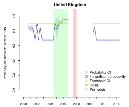
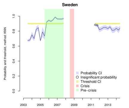
Figure 2: Probabilities and thresholds, and their CIs, of KNN for United Kingdom and Sweden

For UK, the left chart in Figure 2 illustrates first one elevated signal (but no threshold exceedance) already in 2002, and then during the pre-crisis period larger variation in elevated probabilities, which cause an insignificant difference to the threshold and hence an indication of potential vulnerability. This would have indicated vulnerability four quarters earlier than without considering uncertainty. On the other hand, the right chart in Figure 2 shows for Sweden that the two observations after a post-crisis period are elevated but below the threshold. In the correct context, and in conjunction with expert judgment, this would most likely not be related to a boom-bust type of an imbalance, but rather elevated values in the aftermath of a crisis.

As a next step in showing the usefulness of incorporating uncertainty in models, we conduct an early-warning exercise in which we disregard observations whose probabilities $p_{n}^{m}$ and $p_{n}^{a}$ do not statistically significantly differ from thresholds $\tau_{n}^{m}$ and $\tau_{n}^{a}$, respectively. Due to larger data needs in the recursive exercise, which would leave us with small samples, we only conduct a cross-validated horse race of methods, as well as compare it to the exercise in Table 9. In this case, the cross-validated exercise functions well as a test of the impact of disregarding insignificant observations on early-warning performance. In Table 11, rather than focusing on specific rankings of methods, we enable a comparison of the results of the new performance evaluation to the full results in Table 9. With the exception of signal extraction, which anyhow exhibits low Usefulness, we can observe that all methods yield better performance when dropping insignificant observations. While this is intuitive, as the dropped observations are borderline cases, the results mainly function as general-purpose evidence of our model output uncertainty measure and the usefulness of considering statistical significance vis-à-vis thresholds.

Table 11: A robust and significant horse race of cross-validated estimations.

5 Conclusion

This paper has presented first steps toward robust early-warning models. As early-warning models are oftentimes built in isolation of other methods, the exercise is of high relevance for assessing the relative performance of a wide variety of methods.

We have conducted a cross-validated and recursive horse race of conventional statistical and more recent machine learning methods. This provided information on best-performing approaches, as well as an overall ranking of early-warning methods. The value of the horse race descends from its robustness and objectivity. Further, we have tested four structured approaches to aggregating the information products of built early-warning models. Two structured approaches involve choosing the best method (in-sample) for out-of-sample use, and relying on the majority vote of all methods together. Then, moving toward more standard ensemble methods for the use of multiple modeling techniques, we combined model outputs into an arithmetic mean and performance-weighted mean of all methods. Finally, we provided approaches for estimating model uncertainty in early-warning exercises. One approach to tackling model performance uncertainty, and provide robust rankings of methods, is the use of mean-comparison tests on model performance. Also, we allow for testing whether differences among the model output and thresholds are statistically significantly different, as well as show that accounting for this in signaling exercises yields added value. All approaches put forward in this paper have been applied in a European setting, particularly in predicting the still ongoing financial crisis using a broad set of indicators. Generally, our results show that the conventional statistical approaches are outperformed by more advanced machine learning methods, such as $k$-nearest neighbors and neural networks, and particularly by model aggregation approaches through ensemble learning.

The value and implications of this paper are manifold. First, we provide an approach for conducting robust and objective horse races, as well as an application to Europe. In relation to previous efforts, this provides the first objective comparison of model performance, as we assure a similar setting for each method when being evaluated, including data, forecast horizons, post-crisis bias, loss function, policymaker’s preferences and overall exercise implementation. The robustness descends from the use of resampling to assess performance, which assures stable results not only with respect to small variation in data but also for the non-deterministic modeling techniques. In the recursive real-time exercises that control for non-linear function approximators overfitting data, we still find recent machine learning approaches to outperform conventional statistical methods. Beyond showing that machine learning approaches have potential in these types of exercises, this also points to the importance of using appropriate resampling techniques, such as accounting for time dependence. Second, given the number of different available methods, the use of multiple modeling techniques is a necessity in order to collect information of different types of vulnerabilities. This might involve the simultaneous use of multiple models in parallel or some type of aggregation. In addition to improvements in performance and robustness, this may be valuable due to the fact that some of the more recent machine learning techniques are oftentimes seen as opaque in their functioning and less interpretable. For instance, if a majority vote of a panel of models points to a vulnerability, preferences against one individual modeling approach are less of a concern. Thus, as the ensemble models both perform well in horse races and decrease variability in model performance, structured approaches to aggregate model output ought to be one part of a robust early-warning toolbox. Third, even though techniques and data for early-warning analysis are advancing, and so is performance, it is of central importance to understand the uncertainty in models. A key topic is to assure that breaching a threshold is not due to sampling error alone. Likewise, we should be concerned with observations below but close to a threshold, particularly when the difference is not of significant size.

For the future, we hope that a large number of approaches for measuring systemic risk, including those presented herein, are to be implemented in a more structured and user-friendly manner. In particular, a broad palette of measurement techniques requires a common platform for modeling systemic risk and visualizing information products, as well as means to interact with both model parameters and visual interfaces. This could, for instance, involve the use of visualization and interaction techniques provided in the VisRisk platform for visual systemic risk analytics [72], as well as more advanced data and dimension reduction techniques [73, 75]. In conjunction with these types of interfaces, we hope that this paper generally stimulates the simultaneous use of a broad panel of methods, and their aggregates, as well as accounting for uncertainty when interpreting results.

Appendix A Robustness tests and additional results

Table A.1: Cross-validated results for signal extraction.

Table A.2: Cross-validated results for signal extraction with $\mu=0.9193$.

Table A.3: A horse race of recursive real-time estimations with dropped windows.

Table A.4: Aggregated results of recursive estimations with dropped windows.

Table A.5: Significances of cross-validated Usefulness comparisons.

Table A.6: Significances of recursive Usefulness comparisons.

Table A.7: Significances of cross-validated AUC comparisons.

Table A.8: Significances of recursive AUC comparisons.

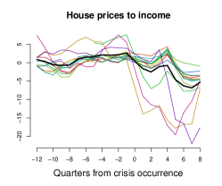
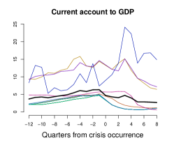
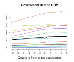
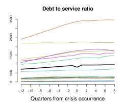
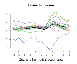
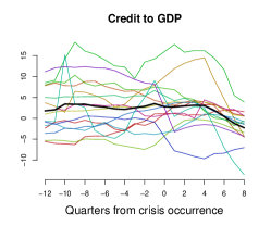
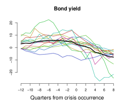
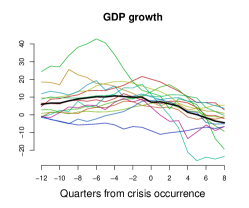
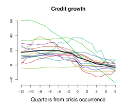
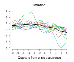
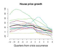
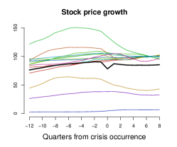
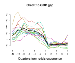
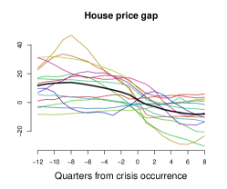
Figure A.1: Plots of each indicator from $t-12$ to $t+8$ around crisis occurrences for each country. The average of all entities is depicted as a bold line.

Figure A.2: Cross-validated out-of-sample ROC curve plots for all methods and the aggregates

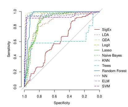
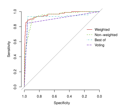
Figure A.3: Recursive out-of-sample ROC curve plots for all methods and the aggregates

References

- Alessi and Detken [2011] L. Alessi and C. Detken. Quasi real time early warning indicators for costly asset price boom/bust cycles: A role for global liquidity. European Journal of Political Economy, 27(3):520–533, 2011.
- Alessi and Detken [2014] L. Alessi and C. Detken. Identifying excessive credit growth and leverage. ECB Working Paper No. 1723, 2014.
- Alessi et al. [2014] L. Alessi, A. Antunes, J. Babecky, S. Baltussen, M. Behn, D. Bonfim, O. Bush, C. Detken, J. Frost, R. Guimaraes, T. Havranek, M. Joy, K. Kauko, J. Mateju, N. Monteiro, B. Neudorfer, T. Peltonen, P. Rodrigues, M. Rusnák, W. Schudel, M. Sigmund, H. Stremmel, K. Smidkova, R. van Tilburg, B. Vasicek, and D. Zigraiova. Comparing different early warning systems: Results from a horse race competition among members of the macro-prudential research network. ECB, mimeo, 2014.
- Altman [1968] E.I. Altman. Financial ratios, discriminant analysis and the prediction of corporate bankruptcy. The Journal of Finance, 23(4):589–609, 1968.
- Altman [1992] N.S. Altman. An introduction to kernel and nearest-neighbor nonparametric regression. The American Statistician, 46(3):175–185, 1992.
- Arlot and Celisse [2010] S. Arlot and A. Celisse. A survey of cross-validation procedures for model selection. Statistical Surveys, 4:40–79, 2010.
- Babecky et al. [2012] J. Babecky, T. Havranek, J. Mateju, M. Rusnak, K. Smidkova, and B. Vasicek. Banking, debt and currency crises: Early warning indicators for developed countries. ECB Working Paper No. 1485, 2012.
- Barrell et al. [2010] R. Barrell, P.E. Davis, D. Karim, and I.. Liadze. Bank regulation, property prices and early warning systems for banking crises in OECD countries. Journal of Banking & Finance, 34(9):2255–2264, 2010.
- Beaver [1966] W. H. Beaver. Financial ratios as predictors of failure. Journal of Accounting Research, 4:71–111, 1966.
- Berg and Pattillo [1999] A. Berg and C. Pattillo. Predicting currency crises – the indicators approach and an alternative. Journal of International Money and Finance, 18(4):561–586, 1999.
- Berg et al. [2005] A. Berg, E. Borensztein, and C. Pattillo. Assessing early warning systems: How have they worked in practice? IMF Staff Papers, 52(3), 2005.
- Borio and Drehmann [2009] C Borio and M. Drehmann. Assessing the risk of banking crises – revisited. BIS Quarterly Review, (March), 2009.
- Breiman [1996a] L. Breiman. Bagging predictors. Machine Learning, 24(2):123–140, 1996a.
- Breiman [1996b] L. Breiman. Heuristics of instability and stabilization in model selection. Annals of Statistics, 24:2350–2383, 1996b.
- Breiman [2001] L. Breiman. Random forests. Machine Learning, 45(1):5–32, 2001.
- Breiman and Spector [1992] L. Breiman and P. Spector. Submodel selection and evaluation in regression: The x-random case. International Statistical Review, 60:291–319, 1992.
- Breiman et al. [1984] L. Breiman, J.H. Friedman, R.A. Olshen, and C.J. Stone. Classification and Regression Trees. Wadsworth, Belmont, CA, 1984.
- Bussière and Fratzscher [2006] M. Bussière and M. Fratzscher. Towards a new early warning system of financial crises. Journal of International Money and Finance, 25(6):953–973, 2006.
- Caprio and Klingebiel [2003] G. Caprio and D. Klingebiel. Episodes of systemic and borderline financial crises. Banking Crisis Database, World Bank, Washington D.C., January 2003, 2003.
- Caprio et al. [2005] G. Caprio, D. Klingebiel, L Laeven, and G. Noguera. Appendix: Banking crisis database", published in. In P. Honohan and L. Laeven, editors, Systemic Financial Crises, pages 307–340. Cambridge: Cambridge University Press, 2005.
- Chamon et al. [2007] M. Chamon, P. Manasse, and A. Prati. Can we predict the next capital account crisis? IMF Staff Papers, 54:270–305, 2007.
- Chu and Marron [1991] C.-K. Chu and J. S. Marron. Comparison of two bandwidth selectors with dependent errors. Annals of Statistics, 19(4):1906–1918, 1991.
- Cortes and Vapnik [1995] C. Cortes and V. Vapnik. Support-vector networks. Machine Learning, 20(3):273–297, 1995.
- Demyanyk and Hasan [2010] Y.S. Demyanyk and I. Hasan. Financial crises and bank failures: A review of prediction methods. Omega, 38(5):315–324, 2010.
- Drehmann et al. [2011] M. Drehmann, C. Borio, and K. Tsatsaronis. Anchoring countercyclical capital buffers: The role of credit aggregates. International Journal of Central Banking, 7(4):189–240, 2011.
- Duttagupta and Cashin [2011] R. Duttagupta and P. Cashin. Anatomy of banking crises in developing and emerging market countries. Journal of International Money and Finance, 30(2):354–376, 2011.
- Efron [1979] B. Efron. Bootstrap methods: Another look at the jackknife. The Annals of Statistics, 7(1):1–26, 1979.
- Efron [1981] B. Efron. Nonparametric estimates of standard error: The jackknife, the bootstrap and other methods. Biometrika, 68:589–599, 1981.
- Efron [1992] B. Efron. Jackknife-after-bootstrap standard errors and influence functions. Journal of the Royal Statistical (Series B), 54:83–127, 1992.
- Efron and Tibshirani [1986] B. Efron and R. Tibshirani. The bootstrap method for standard errors, confidence intervals, and other measures of statistical accuracy. Statistical Science, 1(1):1–35, 1986.
- Efron and Tibshirani [1993] B. Efron and R. Tibshirani. An Introduction to the Bootstrap. Boca Raton, FL: Chapman & Hall/CRC, 1993.
- Eichengreen and Rose [1998] B. Eichengreen and A. K. Rose. Staying afloat when the wind shifts: External factors and emerging-market banking crises. NBER Working Paper, No. 6370, 1998.
- El-Shagi et al. [2013] M. El-Shagi, T. Knedlik, and G. von Schweinitz. Predicting financial crises: The (statistical) significance of the signals approach. Journal of International Money and Finance, 35:76–103, 2013.
- Fioramanti [2008] M. Fioramanti. Predicting sovereign debt crises using artificial neural networks: A comparative approach. Journal of Financial Stability, 4(2):149–164, 2008.
- Fisher [1935] R.A. Fisher. The Design of Experiments. Oliver and Boyd, London, 3rd edition edition, 1935.
- Fisher [1936] R.A. Fisher. The use of multiple measurements in taxonomic problems. Annals of Eugenics, 7(2):179–188, 1936.
- Franck and Schmied [2003] R. Franck and A. Schmied. Predicting currency crisis contagion from east asia to russia and brazil: An artificial neural network approach. IMCB Working Paper No. 2, 2003.
- Frank and Cline [1971] C. Frank and W. Cline. Measurement of debt servicing capacity: An application of discriminant analysis. Journal of International Economics, 1(3):327–344, 1971.
- Frankel and Rose [1996] J. A. Frankel and A. K. Rose. Currency crashes in emerging markets: An empirical treatment. Journal of International Economics, 41(3–3):351–366, 1996.
- Fuertes and Kalotychou [2006] A.-M. Fuertes and E. Kalotychou. Early warning system for sovereign debt crisis: The role of heterogeneity. Computational Statistics and Data Analysis, 5:1420–1441, 2006.
- Hastie et al. [2011] T. Hastie, R. Tibshirani, and J. Friedman. The Elements of Statistical Learning: Data Mining, Inference, and Prediction. Springer, 2011.
- Ho [1995] T. Ho. Random decision forests. In Proceedings of the Third International Conference on Document Analysis and Recognition, pages 278–282, 1995.
- Holopainen and Sarlin [2015] M. Holopainen and P. Sarlin. CrisisModeler: A tool for exploring crisis predictions. In Proceedings of the IEEE Symposium on Computational Intelligence for Financial Engineering & Economics, 2015.
- Hornik et al. [1989] K. Hornik, M. Stinchcombe, and H. White. Multilayer feedforward networks are universal approximators. Neural Networks, 2:359–366, 1989.
- Hounkannounon [2011] B. Hounkannounon. Bootstrap for Panel Data Models with an Application to the Evaluation of Public Policies. PhD thesis, University of Montreal, 2011.
- Huang et al. [2006] G-B. Huang, Q-Y. Zhu, and C-K. Siew. Extreme learning machine: Theory and applications. Neurocomputing, 70:489–501, 2006.
- Hurlin et al. [2013] C. Hurlin, S. Laurent, R. Quaedvlieg, and S. Smeekes. Risk measure inference. Working Paper, HAL Id: halshs-00877279, 2013.
- IMF [2010] IMF. The financial stress index for advanced economies. In World Economic Outlook, 2010.
- Kaminsky [2003] G. Kaminsky. Varieties of currency crises. NBER Working Papers, No. 10193, National Bureau of Economic Research., 2003.
- Kaminsky and Reinhart [1996] G. Kaminsky and C. Reinhart. The twin crises: The causes of banking and balance of payments problems. Federal Reserve Board Discussion Paper, No. 544, 1996.
- Kaminsky et al. [1998] G. Kaminsky, S. Lizondo, and C. Reinhart. Leading indicators of currency crises. IMF Staff Papers, 45(1):1–48, 1998.
- Kapetanios [2008] G. Kapetanios. A bootstrap procedure for panel data sets with many cross-sectional units. Econometrics Journal, 11:377–395, 2008.
- Kindleberger and Aliber [2011] C. Kindleberger and R. Aliber. Manias, Panics and Crashes: A History of Financial Crises, volume Sixth edition. New York: Palgrave Macmillan., 2011.
- Knedlik and von Schweinitz [2012] T. Knedlik and G. von Schweinitz. Macroeconomic imbalances as indicators for debt crises in europe. Journal of Common Market Studies, 50(5):726–745, 2012.
- Künsch [1989] H. R. Künsch. The jackknife and the bootstrap for general stationary observations. The Annals of Statistics, pages 1217–1241, 1989.
- Kohavi [1995] R. Kohavi. A study of cross-validation and bootstrap for accuracy estimation and model selection. In Proceedings of the International Joint Conference on Artificial intelligence, volume 2, pages 1137–1143, San Francisco, CA, USA, 1995. Morgan Kaufmann Publishers Inc.
- Kohavi et al. [1997] R. Kohavi, B. Becker, and D. Sommerfield. Improving simple bayes. In Proceedings of the European Conference on Machine Learning, 1997.
- Kuncheva and Whitaker [2003] L. Kuncheva and C. Whitaker. Measures of diversity in classifier ensembles. Machine Learning, 51:181–207, 2003.
- Laeven and Valencia [2013] L. Laeven and F. Valencia. Banking crisis database: An update. IMF Economic Review, 2013.
- Lainà et al. [2015] P. Lainà, J. Nyholm, and P. Sarlin. Leading indicators of systemic banking crises: Finland in a panel of eu countries. Review of Financial Economics, 2015.
- Lang et al. [2015] J.H. Lang, T. Peltonen, and P. Sarlin. A framework for early-warning modeling. ECB Working Paper Series, forthcoming, 2015.
- Lo Duca and Peltonen [2013] M. Lo Duca and T. A. Peltonen. Assessing systemic risks and predicting systemic events. Journal of Banking & Finance, 37(7):2183–2195, 2013.
- Nag and Mitra [1999] A. Nag and A. Mitra. Neural networks and early warning indicators of currency crisis. Reserve Bank of India Occasional Papers 20(2), 183–222, 1999.
- Peltonen [2006] T.A Peltonen. Are emerging market currency crises predictable? A test. ECB Working Paper No. 571, 2006.
- Quenouille [1949] M.H. Quenouille. Approximate tests of correlation in time series. Journal of the Royal Statistical Society (Series B), 11:68–84, 1949.
- Ramser and Foster [1931] J. Ramser and L. Foster. A demonstration of ratio analysis. Bureau of Business Research, University of Illinois,Urbana, IL, Bulletin 40, 1931.
- Reinhart and Rogoff [2009] C. M. Reinhart and K.S. Rogoff. This time is different: Eight Centuries of Financial Folly. Princeton University Press, Princeton, 2009.
- Ripley [1994] B. Ripley. Neural networks and related methods for classification. Journal of the Royal Statistical Society, 56.:409–456, 1994.
- Sachs et al. [1996] J. Sachs, A. Tornell, and A. Velasco. Financial crises in emerging markets: The lessons from 1995. Brookings Papers on Economic Activity, No. 1:147–218, 1996.
- Sarle [1994] W. Sarle. Neural networks and statistical models. In Proceedings of the Nineteenth Annual SAS Users Group International Conference, pages 1538–1550., Cary, NC: SAS Institute, 1994.
- Sarlin [2013a] P. Sarlin. On biologically inspired predictions of the global financial crisis. Neural Computing and Applications, 24(3–4):663–673, 2013a.
- Sarlin [2013b] P Sarlin. Macroprudential oversight, risk communication and visualization. London School of Economics, Systemic Risk Centre, Special Paper 4, 2013b.
- Sarlin [2013c] P. Sarlin. Exploiting the self-organizing financial stability map. Engineering Applications of Artificial Intelligence, forthcoming, 2013c.
- Sarlin [2013d] P. Sarlin. On policymakers’ loss functions and the evaluation of early warning systems. Economics Letters, 119(1):1–7, 2013d.
- Sarlin [2013e] P. Sarlin. Decomposing the global financial crisis: A self-organizing time map. Pattern Recognition Letters, 34:1701–1709, 2013e.
- Sarlin and Marghescu [2011] P. Sarlin and D. Marghescu. Neuro-genetic predictions of currency crises. Intelligent Systems in Accounting, Finance and Management, 18(4):145–160, 2011.
- Sarlin and Peltonen [2013] P. Sarlin and T. Peltonen. Mapping the state of financial stability. Journal of International Financial Markets, Institutions & Money, 26:46–76, 2013.
- Schapire [1990] R.E. Schapire. The strength of weak learnability. Machine Learning, 5(2):197–227, 1990.
- Schimmelpfennig et al. [2003] A. Schimmelpfennig, N. Roubini, and P. Manasse. Predicting sovereign debt crises. IMF Working Papers 03/221, International Monetary Fund., 2003.
- Schmidt [1984] R. Schmidt. Early warning of debt rescheduling. Journal of Banking & Finance, 8(2):357–370, 1984.
- Shao [1993] J. Shao. Linear model selection by cross-validation. Journal of the American Statistical Association, 88(422):486–494, 1993.
- Stone [1977] M. Stone. Asymptotics for and against cross-validation. Biometrika, 64:29–35, 1977.
- Taffler and Abassi [1984] R. J. Taffler and B. Abassi. Country risk: A model for predicting debt servicing problems in developing countries. Journal of the Royal Statistical Society. Series A (General), 147(4):541–568, 1984.
- Tibshirani [1996] R. Tibshirani. Regression shrinkage and selection via the lasso. Journal of the Royal Statistical Society (Series B), 58(1):267–288, 1996.
- Vanwinckelen and Blockeel [2012] G. Vanwinckelen and H. Blockeel. On estimating model accuracy with repeated cross-validation. In B. De Baets, B. Manderick, M. Rademaker, and W. Waegeman, editors, Proceedings of the 21st Belgian-Dutch Conference on Machine Learning, pages 39–44, Ghent, 2012.
- Venables and Ripley [2002] W.N. Venables and B.D. Ripley. Modern Applied Statistics with S. Fourth edition. Springer., 2002.
- Wolpert [1992] D. H. Wolpert. Stacked generalization. Neural Networks, 5:241–259, 1992.
- Zhang [1993] P. Zhang. Model selection via multifold cross validation. The Annals of Statistics, 21:299–313, 1993.